
Hierarchical Adaptive Eddy-Capturing Approach for Modeling and Simulation of Turbulent Flows


1
Engineering Department, University of Campania Luigi Vanvitelli, Via Roma 29, 81031 Aversa, Italy
2
Keldysh Institute of Applied Mathematics of Russian Academy of Sciences, 125047 Moscow, Russia
3
Adaptive Wavelet Technologies LLC, Superior, CO 80027, USA
*
Author to whom correspondence should be addressed.
Fluids 2021, 6(2), 83; https://0-doi-org.brum.beds.ac.uk/10.3390/fluids6020083
Submission received: 10 January 2021
/
Revised: 8 February 2021
/
Accepted: 9 February 2021
/
Published: 13 February 2021
(This article belongs to the Special Issue Wavelets and Fluid Dynamics)
Abstract
:A short review of wavelet-based adaptive methods for modeling and simulation of incompressible turbulent flows is presented. Wavelet-based computational modeling approaches of different fidelities are recast into an integrated hierarchical adaptive eddy-capturing turbulence modeling framework. The wavelet threshold filtering procedure and the associated wavelet-filtered Navier–Stokes equations are briefly discussed, along with the adaptive wavelet collocation method that is used for numerical computations. Depending on the level of wavelet thresholding, the simulation is possibly supplemented with a localized closure model. The latest advancements in spatiotemporally varying wavelet thresholding procedures along with the adaptive-anisotropic wavelet-collocation method make the development of a fully adaptive approach feasible with potential applications for complex turbulent flows.
1. Introduction
The detailed comparisons of computational fluid dynamics (CFD) results against experimental findings have clearly shown the importance of capturing the dominant three-dimensional flow structures when simulating fluid turbulence (e.g., [1]). For highly turbulent flows, due to the prohibitive computational cost of resolving the whole range of spatial and temporal scales through direct numerical simulation (DNS), the computationally feasible alternative is represented by large-eddy simulation (LES), where only eddies that dominate large-scale flow physics are resolved. However, when dealing with complex turbulent flows, standard LES methodologies rely on, at best, a zonal grid adaptation strategy to attempt to minimize the associated high computational costs. While an improvement over using regular grids, these methodologies fail to resolve the high wavenumber components of the spatially intermittent coherent eddies that typify fluid turbulence. At the same time, the flow results in being over-resolved in regions between the intermittent coherent eddies, with a waste of computational power. The role of coherent and incoherent residual modes in LES modeling was demonstrated in Reference [2], where the coherent/incoherent decomposition of the subgrid-scale (SGS) stresses based on the wavelet de-noising procedure was introduced. A priori dynamical tests based on the perfect modeling approach [3,4] were performed for decaying homogeneous isotropic turbulence (HIT) while evaluating the theoretical effects of SGS forces during the simulation. By examining the relation between deterministic/stochastic SGS models and coherent/incoherent SGS stresses, the main result was that, in LES, low-order statistics can be almost exactly reproduced when only the effect of coherent SGS modes is accounted for, while incoherent SGS modes have a negligible effect upon large-scale dynamics and energy transfer between resolved and unresolved flow structures.
The development of wavelet-based adaptive LES (WA-LES) addresses shortcomings of traditional LES approaches by using a dynamic grid adaptation strategy that resolves energetic coherent eddies regardless of their size. The centerpiece of this approach is the existence of energetic coherent structures that govern turbulent flow dynamics across the full spectral range [5]. This novel methodology, which is based on the application of a wavelet threshold filtering (WTF) procedure, demonstrated the ability to dynamically resolve and track the most energetic part of the coherent turbulent eddies while exploiting a field compression that allows for a significant reduction of the number of grid points used in the numerical computations. Moreover, the principal idea behind WA-LES was taken one step further by introducing the variable wavelet thresholding strategy to locally and temporally maintain the desired level of turbulence resolution. This was achieved by ensuring that only the a priori specified fraction of turbulent kinetic energy, SGS dissipation, or other statistical quantities was resolved. With such a strategy, the transition between wavelet-based adaptive DNS (WA-DNS), coherent vortex simulation (CVS), and WA-LES regimes becomes natural. Therefore, the three different methods can be recast into a wavelet-based hierarchical adaptive eddy-capturing approach for modeling and simulation of turbulent flows, as discussed in this article.
The remainder of the manuscript is organized as follows. The WTF operation and the dynamic grid adaptation procedure are reviewed in Section 2, where the wavelet-filtered incompressible Navier–Stokes equations are introduced, along with the closure model. The hierarchical adaptive eddy-capturing approach is presented in Section 3, where the combined wavelet-collocation/volume-penalization method for simulating wall-bounded turbulent flows is discussed. Finally, some concluding remarks are drawn in Section 4.
2. Wavelet-Filtered Navier–Stokes Equations
2.1. Wavelet Threshold Filtering
The essential component of the present hierarchical adaptive eddy-capturing approach is the multi-resolution wavelet representation of a general scalar field, say , which decomposes the n-dimensional variable in terms of scaling functions () at the coarsest level of resolution, and wavelets () of different families () and levels of resolution (). Namely, this decomposition has the following form:
where the bold subscripts and denote n-dimensional indices while and stand for the associated index sets, and J is the maximum level of resolution that is present or allowed in the wavelet approximation. The scaling functions and the wavelets are constructed on a set of nested tensorial meshes with one-to-one correspondence between grid points and functions. The coefficients and represent, respectively, the averaged values and the local variation details of the field at different scales. Second generation wavelets, for which construction is based on the lifting scheme [6], are employed in decomposition (1). These basis functions are suitable to deal with arbitrary boundary conditions and irregular sampling intervals.
The WTF operation arises naturally from decomposition (1), where wavelets with coefficients falling below a given prescribed limit are discarded. Formally, the corresponding wavelet-filtered quantity, say , can be represented by the following conditional wavelet projection:
in which the terms are a subset of the original projection. Given the number J of resolution levels, the filtered variable thus consists of the relatively more important wavelet modes, according to the prescribed thresholding level. The latter is taken directly proportional to some characteristic amplitude of the original unfiltered quantity, namely, , with the positive dimensionless parameter representing the constant of proportionality. In fact, once the norm is specified, the spatial filtering operator (2) is uniquely defined by the threshold parameter. Following usual implementations, the –norm of the wavelet-filtered solution is employed so that is assumed as the actual dimensional threshold. The wavelet-based approach provides highly controlled a priori error estimation because the reconstruction error of the filtered variable is shown to converge according to
where is a constant of order unity [7].
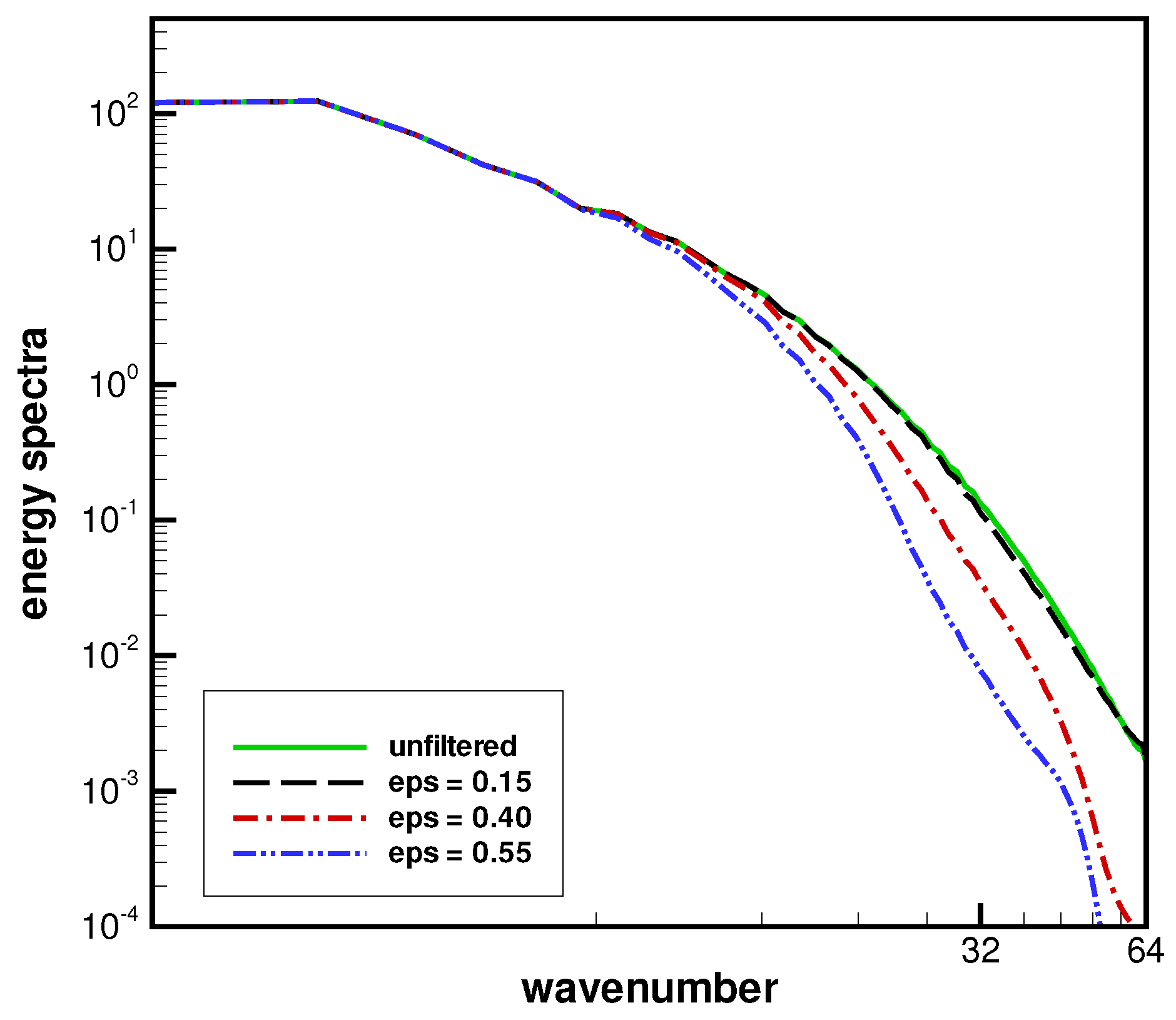
Differently from Fourier cutoff filtering, which is based on functions that are localized in wavenumber space, WTF basis functions are localized in both physical space (due to compact support) and wavenumber space (due to fast decay and vanishing moments). Therefore, WTF can be viewed as a local, spatially variable, smooth filter that removes the high wavenumber components of the flow field. As demonstrated in [8,9], the filter shape significantly affects LES in terms of spectral content and physical interpretation of the solution. In particular, the residual stress tensor strongly depends on the assumed filter shape, which causes closure models to be filter-dependent. The effect of the application of the WTF procedure is illustrated in Figure 1, where the energy spectra associated with filtered HIT velocity fields on a grid are shown [10]. As is expected, the filtering weight increases with the thresholding level.
However, relatively important small-scale flow structures are retained in the filtered solutions, as is also demonstrated in Table 1, where captured energy and enstrophy are examined. The multi-resolution nature of WTF allows small dissipative scales to be partially resolved more effectively than for classical LES filters.
2.2. Filtered Governing Equations
The present article is focused on the hierarchical adaptive approach for modeling and simulation of incompressible turbulent flows. The WA-LES methodology was recently extended to compressible flows [11], as is discussed in the accompanying article in this issue. The incompressible WA-LES-governing equations are formally obtained by applying the WTF operator (2) to the Navier–Stokes equations, together with the divergence free projection. For forced turbulent flows, the filtered equations are formally written as
where and are the constant density and kinematic viscosity of the fluid, while stands for the unfiltered forcing field. The residual SGS stresses
can be thought of as representing the effect of unresolved (less energetic, coherent/incoherent) background flow on the dynamics of resolved (more energetic, coherent) turbulent eddies. Usually, with the isotropic part of the SGS stress tensor being incorporated by a modified pressure variable, only the deviatoric part, hereafter noted with a star, , is modeled. Additionally, the variable does not represent the wavelet-filtered pressure, the bar symbol being only used for consistency reasons. Instead, as is typical for incompressible flows, the pressure term on the right-hand side of (5) has to be viewed in the role of a Lagrange multiplier enforcing the divergence-free velocity condition.
The interpretation of WTF as a spatial low-pass filter highlights the similarity between present WA-LES and classical nonadaptive LES approaches. However, very different from the usual LES filters, WTF continuously changes in time following the resolved flow field. The characteristic filter width, say , which is implicitly defined by the thresholding procedure, results in being a time-dependent pointwise variable parameter. This parameter, which has to be interpreted as the actual turbulence resolution length scale [12], is also a measure of the local numerical resolution, with the minimum allowable characteristic width corresponding to the highest level of resolution J in decomposition (2). The smaller the value of the wavelet threshold , the smaller the length scale and the greater the fraction of resolved kinetic energy.
2.3. Closure Modeling
For any other LES approach, the WA-LES governing equations need to be supplemented by a closure model. The latter is mainly required to provide the right amount of energy dissipation that allows us to mimic the net effect of unresolved turbulent eddies. The local SGS dissipation that is the rate at which energy is locally transferred from energy containing resolved eddies to unresolved residual motions is defined by , with being the resolved strain-rate tensor. For instance, when adopting the eddy-viscosity assumption, , this variable is approximated as , where the turbulent eddy-viscosity has to be determined.
In order to take full advantage of the unique properties of the WA-LES method in simulating complex flows, due to its ability to automatically adapt to the computational mesh, the use of localized models is particularly appropriate. Local dynamic one-equation SGS models based on both eddy-viscosity and non-eddy-viscosity assumptions were developed in [13], where an additional field variable representing the kinetic energy associated with the unresolved motions, , was introduced. Following this approach, the wavelet-filtered incompressible Navier–Stokes equations are numerically solved along with the additional evolution equation for , which can be written as [14]
where the viscous dissipation rate of SGS kinetic energy is suitably modeled [13]. In the framework of localized dynamic kinetic-energy model (LDKM), it is assumed that , and the SGS model can be written as
where the model coefficient is determined through a dynamic procedure. This way, the energy transfer between resolved and residual flow structures can be explicitly taken into account by the closure model without the equilibrium assumption that is often made in classical approaches. It is worth noting that the turbulent eddy-viscosity can locally assume positive as well as negative values, thus allowing for the representation of both direct and reverse energy transfer at the local level. Different from a stochastic formulation of energy backscatter, such as that proposed in [15], the present WA-LES is based on the dynamic procedure utilizing the deterministic eddy-viscosity model. Furthermore, a class of Lagrangian models based on a modified Germano-like dynamic procedure, redefined in terms of WTF procedures, was developed in [16]. These models extend the original path-line formulation for classical LES [17] to either path-line diffusive or path-tube averaging procedures for WA-LES.
2.4. Adaptive Wavelet Collocation Method
From the mathematical point of view, once a model for the SGS stresses is given and suitable initial and boundary conditions are provided, the WA-LES governing equations could be solved using any numerical method. In practice, the filtered momentum in Equation (5) is solved using the adaptive wavelet collocation (AWC) method, where the same WTF procedure is exploited to automatically adapt the computational grid to the numerical solution in both location and scale [18]. The AWC method is an adaptive high-order numerical method for solving problems with localized structures that is based on second-generation wavelets, which allow the order of the wavelets to be varied easily [19].
The dynamic grid adaptation is tightly coupled to the WTF definition (2), owing to the one-to-one correspondence between wavelets in computational space and grid nodes in physical space. As wavelet modes are discarded in the wavelet projection, their respective collocation points are omitted from the computational grid because the associated value of can be reconstructed (interpolated) using the retained wavelets only. It is worth noting that the WTF operation and, therefore, the wavelet-based interpolation, are not positivity preserving. The AWC method is based on the adaptive wavelet transform that is thoroughly discussed in [18,19]. A reconstruction check procedure is also included to ensure that all the ancestry grid points, necessary to perform the forward wavelet transform, are present and that the filtered field is exactly reconstructed from the values on the sparse grid. The spatial mesh results in being locally refined in the regions of strong flow structures while appearing coarser in the regions of low variation because the retained wavelet modes capture energetic coherent eddies. Additionally, since WTF only acts by removing points, the time-dependent mesh adaptation is obtained by predicting AWC points that may become significant during the next time step. The sparse grid that supports is thus enlarged by adding the adjacent zone, namely, the nearest neighbors to each significant collocation point on the current, next lower, and next higher levels of resolution. This strategy practically corresponds to adopting a Courant–Friedrich–Lewy (CFL) condition [20], where a time step limitation for the finite-rate transfer of information is imposed in both the physical and wavenumber spaces. More precisely, the overall grid adaptation process for the numerical solution of the wavelet-filtered equations consists of the following four steps:
- (i)
- given a known solution at the current computational grid, say , the associated wavelet coefficients are computed through forward wavelet transform;
- (ii)
- the mask consisting of the AWC points associated with the retained wavelets (with coefficients for which the moduli are above the prescribed threshold) is created;
- (iii)
- the extended mask is generated by adding the AWC points corresponding to adjacent wavelets (for which the coefficients can potentially become significant during the next time step); and
- (iv)
- the recursive reconstruction check procedure is performed on the extended mask , ensuring that all the ancestry points, necessary to perform the forward wavelet transform on the updated computational grid , are present.
The successive application of wavelet filtering and grid adaptation across time effectively tracks and resolves the evolution of important flow structures on a near-optimal adaptive computational grid [19]. The local resolution length scale can be extracted from the actual global mask during the simulation. For fluid flow problems involving different variables of interest, given the relative level of thresholding, each variable is filtered with its own absolute threshold. In this case, the union of the different AWC grids associated with each variable is used in the role of the actual computational grid. For instance, when employing the LDKM procedure, the adaptation process also takes into account the evolution of the SGS energy variable. Moreover, the possibility of employing control and proxy variables for grid adaptation can be exploited to ensure that all the desired aspects of the solution for associated analyses are maintained during the simulation given the prescribed fidelity. Regarding the time-integration procedure, a multi-step pressure correction method is employed for the integration of (5) with the continuity constraint (4), with the resulting Poisson equation being solved using the AWC elliptic solver developed in [21].
According to the present implicit filtering formulation, derivation of the WA-LES governing equations directly depends on the WTF definition because the built-in filtering effect of the AWC method is exploited. As an alternative, an additional explicit WTF operation could be superimposed during the solution process [22]. This way, the resolved turbulent field is still represented by the filtered variables at the prescribed level of turbulence resolution while the explicit filtering procedure is simply a tool that enables us to use a lower thresholding level for the numerical grid adaptation. However, the use of such an approach results in using additional computational modes beyond the ones that are strictly necessary to achieve the desired goal. For purely implicit filtering, as is done in the present work, the threshold parameter controls both the spatial filter resolution and the numerical accuracy of the solution. In fact, the adaptive mesh in physical space, which corresponds to the retained modes in wavelet space, is employed to distinguish between the relative energy content of the resolved flow structures as well as to determine their scale.
Different from wavelet Galerkin methods that solve problems in wavelet space (e.g., [23]), the AWC method solves the governing equations in physical space. For the results reported in this work, derivative approximations are provided by multi-level central fourth-order finite difference (FD) schemes at the local adaptive resolution level. When the finite differencing stencil requires points that are not explicitly present on the actual collocation grid, the corresponding values are interpolated from the underlying wavelet basis functions. The linearized Crank–Nicolson split-step time-integration method with adaptive time stepping and the parallel version of the AWC solver are employed [24].
It should be mentioned that, as in classical LES with nonuniform filter width, there is a commutation error between the WTF and derivative operators, the effect of which is not explicitly considered. However, this error is significantly reduced by using the adjacent zone for grid adaptation. Moreover, the recent development of the anisotropic AWC method [25] allows us to overcome the geometric restriction associated with the use of second-generation wavelets that require a topologically regular, rectilinear grid. This way, curvilinear mesh geometries can be used, when appropriate, in order to optimize the computational cost of the simulations. Note that the anisotropic extension of the AWC method, however, preserves the characteristic error control of wavelet-based approaches.
2.5. Homogeneous Turbulence Simulation
In this section, to demonstrate the capabilities of the method, the simulation of linearly forced HIT at (based on the Taylor micro-scale ) is briefly discussed [26]. The initial velocity field for the numerical simulations was obtained by wavelet filtering a fully de-aliased pseudo-spectral DNS solution [2]. Due to the polynomial nature of the AWC solver, the maximum resolution was increased with respect to DNS in order not to alter the initial energy content, namely, WA-LES was performed using a maximum resolution with AWC points. However, only a very low fraction of these points was used by WA-LES, which was conducted at , as suggested by the results of past simulations carried out at comparable Reynolds numbers [27].
It was shown that the results of WA-LES with two different SGS models closely match the reference DNS data, using only about of the corresponding nonadaptive computational nodes. In contrast to classical nonadaptive LES, where the energetic small scales are poorly simulated, WA-LES is able to resolve coherent energetic eddies of any size, so that the dynamically important small-scale turbulence is represented. The reference LES solution was obtained by employing the same FD code without grid adaptation, supplied with the global dynamic Smagorinsky eddy-viscosity model. The reference wavelet-filtered DNS solution was obtained by applying the WTF procedure with the same level of thresholding to the DNS data. As was reported in [26], a good agreement was achieved for low-order statistics, such as spectral distributions of energy and enstrophy, all the way down to the dissipative scales.
This is illustrated in Figure 2, where the time-averaged energy and enstrophy spectra for WA-LES with a maximum resolution of are reported. By making a comparison with wavelet-filtered DNS, which stands for the ideal solution, one can conclude that WA-LES is able to represent highest wavenumber modes much better than nonadaptive LES. Instantaneous description of the wavelet-filtered velocity field given in Section 2.1 is thus confirmed for the time-dependent WA-LES solution. Moreover, the good agreement between the no-model WA-LES and wavelet-filtered DNS is not surprising. Indeed, thanks to the adaptive nature of the WA-LES approach, in the absence of modeled dissipation, the energy is transferred to smaller scales all the way down to the Kolmogorov scale, where it is eventually dissipated by viscous stresses. The number of active wavelets for the no-model solution is higher with respect to the modeled cases, and the simulation automatically tends towards a more computationally expensive regime, as is discussed in the following section.
3. Hierarchical Adaptive Eddy-Capturing Approach
The nature and importance of the residual stresses (6) in the wavelet-filtered Navier–Stokes equations depends on the WTF weight, which is determined by the prescribed level of thresholding. For very small thresholds, filtered and unfiltered solutions practically coincide and the SGS stresses are completely negligible. The AWC method is still used for dynamical grid adaptation, and the approach can be referred to as wavelet-based adaptive direct numerical simulation (WA-DNS). The advantage of WA-DNS with respect to traditional DNS, in terms of computational savings, comes from the high compression property of wavelet-based computational modeling.
As demonstrated in a number of different applications, the additional cost associated with the AWC method, with respect to corresponding nonadaptive methods, is more than compensated for by the very high number of discarded AWC grid points during the simulation (e.g., [27]). In fact, when making a fair comparison, the increased per-point computational cost of the AWC solution, which is about four times higher, must be taken into account. However, based on the grid compression observed in both WA-DNS and WA-LES for a variety of flow configurations, the cost of corresponding nonadaptive calculations would undoubtedly be considerably higher. In addition, the wavelet-based approach becomes more and more effective with the increase in the Reynolds number [28].
For slightly larger thresholds, the CVS approach is obtained [29], where the residual field was shown to be close to Gaussian white noise, so that the SGS dissipation is practically negligible and no closure model is needed [30]. It is important to note that there is still significant energy transfer between the resolved and unresolved modes in CVS, but the net energy transfer is practically zero. This approach, which practically corresponds to thresholds chosen according to the de-nosing criteria of Donoho and Johnstone [31], has been shown to recover low-order and some high-order flow statistics [32]. If other high-order statistics are required, then a purely stochastic SGS model may be used. For instance, the HIT energy decay for CVS was demonstrated to be nearly identical to DNS by retaining less than of the wavelet modes [27]. Moreover, the skewness of the first velocity derivative was maintained to within of the DNS value, reflecting the fact that CVS resolves most of the energy dissipation, thus confirming that the total SGS dissipation is substantially negligible. Additionally, the CVS energy spectrum was proven to match the DNS one over the full range of wavenumbers.
Finally, for even larger thresholds, the SGS field is no longer completely incoherent and the effect of coherent residual modes must be modeled through deterministic SGS modeling, which corresponds to the WA-LES approach. The range of the thresholding parameter that works well for the different fidelity methods depends on the flow problem under consideration. For instance, WA-DNS of HIT at can be conducted for , CVS corresponds to the range of , and higher threshold values are used for WA-LES.
Even though the thresholding level is usually assumed as a constant parameter that is prescribed a priori, the use of a global thresholding criterion can represent a limitation of the wavelet-based methods, especially for unsteady, inhomogeneous, and wall-bounded flows. Indeed, in order to maintain the desired level of turbulence resolution, the threshold at which decomposition (2) is truncated should be consistent with the actual flow conditions, where the energy content of the dominant flow structures can significantly vary. Based on this argument, a more sophisticated variable threshold strategy was developed. An example of a fully adaptive eddy-capturing approach based on WTF with time-varying thresholding is described in Reference [10]. With variable thresholding, the instantaneous threshold is automatically adjusted to maintain the turbulence resolution at the a priori prescribed level, which is achieved by solving a simple feedback control equation. In this context, the turbulence resolution parameter that is defined as the ratio between the modeled and the total dissipations serves as an objective measure to classify and compare different LES solutions [33]. The smaller the value of , the smaller the fraction of energy dissipation that is modeled and the smaller this ratio. The time varying threshold method was successfully tested for both linearly forced and freely decaying HIT.
The spatiotemporally adaptive turbulence simulation framework that was further developed in [34] is based on a variable-fidelity representation that tightly integrates numerics with turbulence modeling and aims to capture the flow physics on a near-optimal adaptive mesh. The integration is achieved by combining wavelet-based computational modeling with spatially and temporally varying wavelet thresholding. This strategy provides an automatic smooth transition from directly resolving all flow physics (WA-DNS) to capturing the whole coherent part of the turbulence (CVS), and to resolving only energetic coherent structures (WA-LES). Therefore, a hierarchical adaptive approach is attained, where the switch between different fidelity solutions is achieved by employing a two-way feedback mechanism between the modeled dissipation and the local grid resolution, owing to the spatiotemporal variation of the WTF strength. This way, the proposed methodology systematically accounts for and exploits the characteristic spatiotemporal intermittency of turbulent flows. The procedure consists of tracking the wavelet threshold variable within a Lagrangian frame by exploiting a path-line diffusive averaging approach [16]. The method is based on the solution of the following evolution equation for the threshold field:
To guarantee the smoothness of the spatially varying threshold while maintaining the prescribed level of turbulence resolution, through a suitably constructed forcing term , a Smagorinsky-like diffusion parameter is assumed, namely, , with being a dimensionless coefficient of order unity. For computational efficiency, instead of directly solving Equation (9), the threshold evolution can be also simulated by exploiting the linear interpolation along characteristics, similarly to what proposed in [17]. This procedure was empirically proven to be less expensive in [34].
Note that the same spatiotemporally variable thresholding strategy to resolve and capture energy-containing/dynamically important eddies can be used across the different WA-DNS, CVS, and WA-LES regimes. To highlight this commonality, the developed variable-fidelity framework is referred to as a hierarchical adaptive eddy-capturing approach. The developed methodology was tested for linearly forced HIT at different Reynolds numbers and was demonstrated to effectively control turbulence resolution at the desired time-varying level [34].
Combined Wavelet-Collocation/Volume-Penalization Method
To expand the applicability of the hierarchical adaptive eddy-capturing approach to flows of engineering interest, it was combined with the Brinkman volume penalization method in order to impose wall boundary conditions on solid obstacles [35]. A distinctive advantage of combining wavelet-based dynamic grid adaptation and volume penalization resides in the capability to enforce boundary conditions with a specified accuracy without a significant computational overhead. In fact, the combined approach allows for a significant cost reduction in time associated with grid generation as well as in other computational costs.
By applying the combined approach, the simulation of the turbulent flow past a solid obstacle was considered in [36,37]. The application of the WTF operator (2) to the penalized momentum equations results in the following penalized equation for the wavelet-filtered perturbation velocity:
where represents the freestream velocity, which is given and known. The last term on the right-hand side of this equation mimics the presence of a stationary obstacle, where stands for the mask function associated with the penalized region, say ,
The original equations in the fluid region are solved together with the penalized equations in the solid region. The crucial parameter for the volume-penalization technique is represented by the positive constant , which has the dimension of time and reflects the fictitious porosity of the obstacle. For vanishing , the solution of the penalized Equation (10), supplied with the divergence-free velocity condition (4), converges to the solution of the original equations (without the penalized term), with the global penalty error theoretically scaling with the square root of this parameter [38]. Additionally, since the penalization constant can be prescribed independently of the numerical discretization, the wall boundary condition can be enforced to any desired level of accuracy.
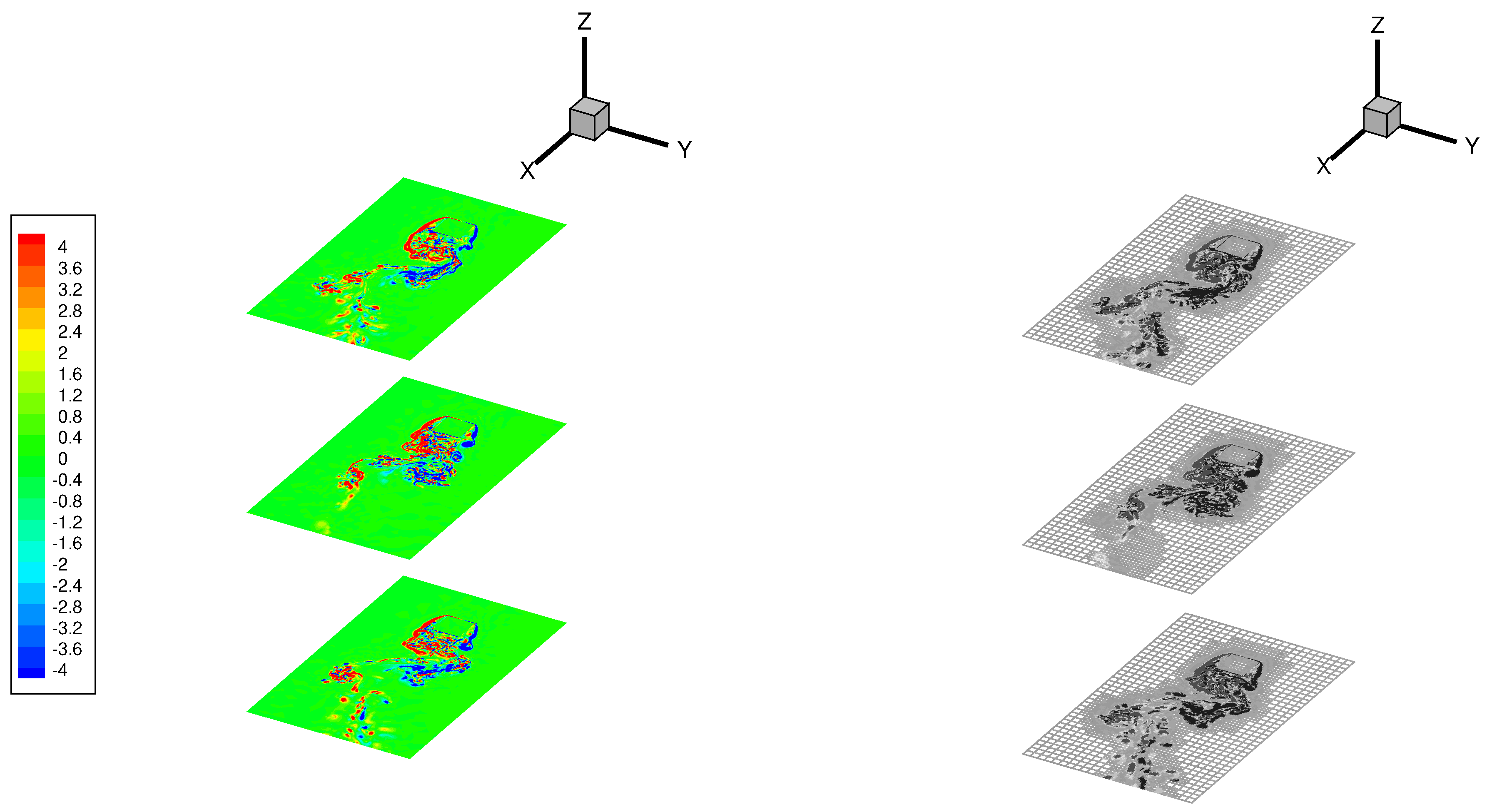
In the following, application of the combined wavelet-collocation/volume-penalization approach to the flow around an isolated stationary prism with square cross-section is discussed. The variable thresholding strategy was successfully tested in Reference [37], whereas the combined approach with constant thresholding was applied to the same geometry in Reference [36]. Depending on the Reynolds number of the flow, either WA-DNS or WA-LES with LDKM was performed. At low supercritical Reynolds number, the wake developed fundamental three-dimensional flow structures for the adaptive method to effectively be able to identify and follow. For example, let us illustrate the WA-LES solution at (based on the square side length H). The flow structure in the near wake () is visualized in Figure 3, wherein the instantaneous contours of the spanwise vorticity are reported at three different planes along the spanwise homogeneous direction. Note that the X-axis corresponds to the inlet flow direction while the Z-axis coincides with the symmetry axis of the cylinder.
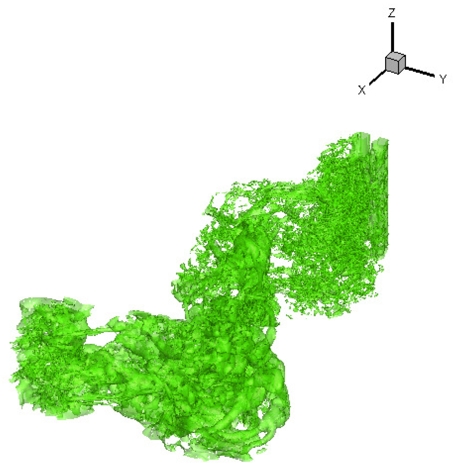
The capability of the present method to dynamically adapt to the fluid flow evolution is clearly demonstrated by looking at the corresponding computational mesh, which is reported on the right side of the same figure. In fact, the active grid points are only present in the regions of large gradients or small-scale flow features, and their instantaneous spatial distribution closely resembles the main vortical structures. That is consistent with the spatiotemporal evolution of the wavelet threshold that adapts to the local flow conditions, with the solution tending towards the desired resolution goal. The three-dimensional structure of the threshold field is visualized in Figure 4, where the instantaneous iso-surfaces of are shown.
The general agreement of the WA-DNS and WA-LES results with the experimental findings and reference numerical nonadaptive solutions, as discussed in References [36,37], demonstrates the feasibility, accuracy, and efficiency of the combined wavelet-collocation/volume-penalization methodology for modeling bluff body flows. For the sake of brevity, only some very important integral results are discussed in this review. In Table 2, the mean drag coefficient and the Strouhal number , associated with the vortex shedding process behind the cylinder, are presented. The results provided by WA-DNS at and WA-LES at were compared with reference numerical data [39,40] as well as experimental findings [41,42]. For each study, the spanwise extent and the solid blockage of the confined flow are also shown.
The effect of varying the thresholding level was examined for WA-DNS at and is presented in Table 3, where the root-mean-square values of the aerodynamic coefficients are also reported. In this case, the WTF level practically stands for a numerical resolution parameter directly affecting the accuracy of the solution. Note that the use of smaller values of the wavelet threshold results in more accurate simulations, with a possible decrease in the minimum mesh spacing at the expense of increasing the number of retained AWC points.
4. Concluding Remarks
The development of wavelet methods in computational fluid mechanics combined with the distinctive capability of wavelet multi-resolution analysis to identify and isolate coherent eddies allows for the integration of numerics- and physics-based turbulence modeling, where energetic flow structures are dynamically tracked on adaptive computational meshes.
This manuscript, while providing a short review of different wavelet-based methods for incompressible turbulence, discusses a novel integrated hierarchical adaptive eddy-capturing approach capable of performing variable fidelity numerical simulations of turbulent flows, including complex geometry applications. However, some further developments are needed before the methodology can be used as a practical tool for simulating turbulent flows of industrial relevance. In particular, higher-Reynold-number flows must be considered, where the adaptive wavelet-based methods are expected to become even more efficient.
The present hierarchical approach is based on utilization of the AWC method for solving the wavelet-filtered governing equations. However, the same wavelet-based method can be also limited to the efficient solution of differently modeled equations. For instance, lower-fidelity approaches such as wavelet-based adaptive unsteady Reynolds-averaged Navier–Stokes (WA-URANS) [43,44,45] and wavelet-based adaptive delayed detached eddy simulation (WA-DDES) [46] were recently developed and incorporated into the more general hierarchical adaptive eddy-resolving framework for wall-bounded compressible turbulent flows, which also includes WA-DNS, CVS, and WA-LES. Differently from the hierarchical adaptive eddy-capturing approach described in this article, the hierarchical adaptive eddy-resolving framework discussed in the accompanying article in this issue also includes model-form adaptation while incorporating both wavelet-filtered and RANS equations, together with the associated model closure equations. Note that both formulations exploit the positive characteristics of wavelet-based numerical methods and achieve significant computational savings from wavelet-based grid compression.
Author Contributions
Data curation, G.D.S. and O.V.V.; investigation, G.D.S. and O.V.V.; methodology, G.D.S. and O.V.V.; resources, G.D.S. and O.V.V.; supervision, G.D.S.; validation, G.D.S. and O.V.V.; visualization, G.D.S.; writing—original draft preparation, G.D.S.; writing—review and editing, G.D.S. and O.V.V. Both authors have read and agreed to the published version of the manuscript.
Funding
This research received no external funding.
Conflicts of Interest
The authors declare no conflict of interest.
Abbreviations
The following abbreviations are used in this manuscript:
| CFD | Computational Fluid Dynamics |
| DNS | Direct Numerical Simulation |
| LES | Large-Eddy Simulation |
| SGS | Sub-Grid Scale |
| HIT | Homogeneous Isotropic Turbulence |
| WA-LES | Wavelet-based Adaptive Large-Eddy Simulation |
| WTF | Wavelet Threshold Filtering |
| WA-DNS | Wavelet-based Adaptive Direct Numerical Simulation |
| CVS | Coherent Vortex Simulation |
| LDKM | Localized Dynamic Kinetic-energy Model |
| AWC | Adaptive Wavelet Collocation |
| CFL | Courant–Friedrich–Lewy |
| FD | Finite Difference |
| GDM | Global Dynamic Model |
| WA-URANS | Wavelet-based Adaptive Unsteady Reynolds-Averaged Navier–Stokes |
| WA-DDES | Wavelet-based Adaptive Delayed Detached Eddy Simulation |
References
- Jimenez, J.; Wray, A.; Saffman, P.; Rogallo, R. The structure of intense vorticity in isotropic turbulence. J. Fluid Mech. 1993, 225, 65–90. [Google Scholar] [CrossRef] [Green Version]
- De Stefano, G.; Goldstein, D.E.; Vasilyev, O.V. On the role of subgrid-scale coherent modes in large-eddy simulation. J. Fluid Mech. 2005, 525, 263–274. [Google Scholar] [CrossRef] [Green Version]
- De Stefano, G.; Vasilyev, O.V. “Perfect” modeling framework for dynamic SGS model testing in large eddy simulation. Theor. Comput. Fluid Dyn. 2004, 18, 27–41. [Google Scholar] [CrossRef]
- De Stefano, G.; Vasilyev, O.V.; Goldstein, D.E. A-priori dynamic test for deterministic/stochastic modeling in large-eddy simulation of turbulent flow. Comput. Phys. Commun. 2005, 169, 10–13. [Google Scholar] [CrossRef]
- Vincent, A.; Meneguzzi, M. The spatial structure and statistical properties of homogeneous turbulence. J. Fluid Mech. 1991, 225, 1–20. [Google Scholar] [CrossRef]
- Sweldens, W. The lifting scheme: A construction of second generation wavelets. SIAM J. Math. Anal. 1998, 29, 511–546. [Google Scholar] [CrossRef] [Green Version]
- Donoho, D.L. Interpolating Wavelet Transforms; Technical Report 3; Preprint; Department of Statistics, Stanford University: Stanford, CA, USA, 1992. [Google Scholar]
- De Stefano, G.; Denaro, F.M.; Riccardi, G. High-order filtering for control volume flow simulation. Int. J. Numer. Methods Fluids 2001, 37, 797–835. [Google Scholar] [CrossRef]
- De Stefano, G.; Vasilyev, O.V. Sharp cutoff versus smooth filtering in large eddy simulation. Phys. Fluids 2002, 14, 362–369. [Google Scholar] [CrossRef] [Green Version]
- De Stefano, G.; Vasilyev, O.V. A fully adaptive wavelet based approach to homogeneous turbulence simulation. J. Fluid Mech. 2012, 695, 149–172. [Google Scholar] [CrossRef]
- De Stefano, G.; Brown-Dymkoski, E.; Vasilyev, O.V. Wavelet-based adaptive large-eddy simulation of supersonic channel flow. J. Fluid Mech. 2020, 901, A13. [Google Scholar] [CrossRef]
- Pope, S. Ten questions concerning the large-eddy simulation of turbulent flows. New J. Phys. 2004, 6, 1–24. [Google Scholar] [CrossRef] [Green Version]
- De Stefano, G.; Vasilyev, O.V.; Goldstein, D.E. Localized dynamic kinetic-energy-based models for stochastic coherent adaptive large eddy simulation. Phys. Fluids 2008, 20, 045102. [Google Scholar] [CrossRef] [Green Version]
- Ghosal, S.; Lund, T.S.; Moin, P.; Akselvoll, K. A dynamic localization model for large-eddy simulation of turbulent flows. J. Fluid Mech. 1995, 286, 229. [Google Scholar] [CrossRef]
- Carati, D.; Ghosal, S.; Moin, P. On the representation of backscatter in dynamic localization models. Phys. Fluids 1995, 7, 606–616. [Google Scholar] [CrossRef]
- Vasilyev, O.V.; De Stefano, G.; Goldstein, D.E.; Kevlahan, N.K.R. Lagrangian dynamic SGS model for stochastic coherent adaptive large eddy simulation. J. Turbul. 2008, 9, 1–11. [Google Scholar] [CrossRef] [Green Version]
- Meneveau, C.; Lund, T.S.; Cabot, W.H. A Lagrangian dynamic subgrid-scale model of turbulence. J. Fluid Mech. 1996, 319, 353–385. [Google Scholar] [CrossRef] [Green Version]
- Vasilyev, O.V.; Bowman, C. Second generation wavelet collocation method for the solution of partial differential equations. J. Comput. Phys. 2000, 165, 660–693. [Google Scholar] [CrossRef] [Green Version]
- Vasilyev, O.V. Solving multi-dimensional evolution problems with localized structures using second generation wavelets. Int. J. Comput. Fluid Dyn. 2003, 17, 151–168. [Google Scholar] [CrossRef]
- Courant, R.; Friedrichs, K.; Lewy, H. Über die partiellen differenzengleichungen der mathematischen physik. Math. Ann. 1928, 100, 32–74. [Google Scholar] [CrossRef]
- Vasilyev, O.V.; Kevlahan, N.K.R. An adaptive multilevel wavelet collocation method for elliptic problems. J. Comput. Phys. 2005, 206, 412–431. [Google Scholar] [CrossRef] [Green Version]
- De Stefano, G.; Vasilyev, O.V. Wavelet-based adaptive large-eddy simulation with explicit filtering. J. Comput. Phys. 2013, 238, 240–254. [Google Scholar] [CrossRef]
- Fröhlich, J.; Schneider, K. An adaptive wavelet Galerkin algorithm for one-dimensional and 2-dimensional flame computations. Eur. J. Mech. B Fluids 1994, 13, 439–471. [Google Scholar]
- Nejadmalayeri, A.; Vezolainen, A.; Brown-Dymkoski, E.; Vasilyev, O.V. Parallel adaptive wavelet collocation method for PDEs. J. Comput. Phys. 2015, 298, 237–253. [Google Scholar] [CrossRef] [Green Version]
- Brown-Dymkoski, E.; Vasilyev, O.V. Adaptive-anisotropic wavelet collocation method on general curvilinear coordinate systems. J. Comput. Phys. 2017, 333, 414–426. [Google Scholar] [CrossRef] [Green Version]
- De Stefano, G.; Vasilyev, O.V. Stochastic coherent adaptive large eddy simulation of forced isotropic turbulence. J. Fluid Mech. 2010, 646, 453–470. [Google Scholar] [CrossRef]
- Goldstein, D.E.; Vasilyev, O.V.; Kevlahan, N.K.R. CVS and SCALES simulation of 3-D isotropic turbulence. J. Turbul. 2005, 6, 1–20. [Google Scholar] [CrossRef]
- Nejadmalayeri, A.; Vezolainen, A.; Vasilyev, O.V. Reynolds number scaling of coherent vortex simulation and stochastic coherent adaptive large eddy simulation. Phys. Fluids 2013, 25, 110823. [Google Scholar] [CrossRef] [Green Version]
- Farge, M.; Schneider, K.; Kevlahan, N.K.R. Non-gaussianity and coherent vortex simulation for two-dimensional turbulence using an adaptive orthogonal wavelet basis. Phys. Fluids 1999, 11, 2187–2201. [Google Scholar] [CrossRef] [Green Version]
- Farge, M.; Pellegrino, G.; Schneider, K. Coherent vortex extraction in 3d turbulent flows using orthogonal wavelets. Phys. Rev. Lett. 2001, 87, 054501. [Google Scholar] [CrossRef] [PubMed] [Green Version]
- Donoho, D.L.; Johnstone, I.M. Ideal Spatial Adaptation via Wavelet Shrinkage. Biometrika 1994, 81, 425–455. [Google Scholar] [CrossRef]
- Schneider, K.; Farge, M.; Pellegrino, G.; Rogers, M. Coherent vortex simulation of three-dimensional turbulent mixing layers using orthogonal wavelets. J. Fluid Mech. 2005, 534, 39–66. [Google Scholar] [CrossRef] [Green Version]
- Geurts, B.J.; Frohlich, J. A framework for predicting accuracy limitations in large-eddy simulation. Phys. Fluids 2002, 14, L41–L44. [Google Scholar] [CrossRef] [Green Version]
- Nejadmalayeri, A.; Vezolainen, A.; De Stefano, G.; Vasilyev, O.V. Fully adaptive turbulence simulations based on Lagrangian spatio-temporally varying wavelet thresholding. J. Fluid Mech. 2014, 749, 794–817. [Google Scholar] [CrossRef] [Green Version]
- Angot, P.; Bruneau, C.H.; Fabrie, P. A penalization method to take into account obstacles in viscous flows. Numer. Math. 1999, 81, 497–520. [Google Scholar] [CrossRef]
- De Stefano, G.; Vasilyev, O.V. Wavelet-based adaptive simulations of three-dimensional flow past a square cylinder. J. Fluid Mech. 2014, 748, 433–456. [Google Scholar] [CrossRef] [Green Version]
- De Stefano, G.; Nejadmalayeri, A.; Vasilyev, O.V. Wall-resolved wavelet-based adaptive large-eddy simulation of bluff-body flows with variable thresholding. J. Fluid Mech. 2016, 788, 303–336. [Google Scholar] [CrossRef]
- Carbou, G.; Fabrie, P. Boundary layer for a penalization method for viscous incompressible flow. Adv. Differ. Equ. 2003, 8, 1409–1532. [Google Scholar]
- Sohankar, A.; Norberg, C.; Davidson, L. Simulation of three-dimensional flow around a square cylinder at moderate Reynolds numbers. Phys. Fluids 1999, 11, 288–306. [Google Scholar] [CrossRef]
- Brun, C.; Aubrun, S.; Goossens, T.; Ravier, P. Coherent structures and their frequency signature in the separated shear layer on the sides of a square cylinder. Flow Turbul. Combust. 2008, 81, 97–114. [Google Scholar] [CrossRef]
- Luo, S.C.; Chew, Y.T.; Ng, Y.T. Characteristics of square cylinder wake transition flows. Phys. Fluids 2003, 15, 2549–2559. [Google Scholar] [CrossRef]
- Lyn, D.A.; Rodi, W. The flapping shear layer formed by flow separation from the forward of a square cylinder. J. Fluid Mech. 1994, 267, 353–376. [Google Scholar] [CrossRef]
- De Stefano, G.; Vasilyev, O.V.; Brown-Dymkoski, E. Wavelet-based adaptive unsteady Reynolds-averaged turbulence modelling of external flows. J. Fluid Mech. 2018, 837, 765–787. [Google Scholar] [CrossRef]
- Ge, X.; Vasilyev, O.V.; De Stefano, G.; Hussaini, M.Y. Wavelet-based adaptive unsteady Reynolds-averaged Navier-Stokes computations of wall-bounded internal and external compressible turbulent flows. In Proceedings of the 2018 AIAA Aerospace Sciences Meeting, Kissimmee, FL, USA, 8–12 January 2018. AIAA Paper 2018–0545. [Google Scholar]
- Ge, X.; Vasilyev, O.V.; De Stefano, G.; Hussaini, M.Y. Wavelet-based adaptive unsteady Reynolds-Averaged Navier-Stokes simulations of wall-bounded compressible turbulent flows. AIAA J. 2020, 58, 1529–1549. [Google Scholar] [CrossRef]
- Ge, X.; Vasilyev, O.V.; Hussaini, M.Y. Wavelet-based adaptive delayed detached eddy simulations for wall-bounded compressible turbulent flows. J. Fluid Mech. 2019, 873, 1116–1157. [Google Scholar] [CrossRef]
Figure 1.
Energy spectra for a wavelet-filtered instantaneous velocity field with different thresholding levels along with the unfiltered solution.
Figure 1.
Energy spectra for a wavelet-filtered instantaneous velocity field with different thresholding levels along with the unfiltered solution.

Figure 2.
Forced homogeneous isotropic turbulence (HIT): time-averaged energy (left) and enstrophy (right) spectra for wavelet-based adaptive large-eddy simulation (WA-LES) with localized dynamic kinetic-energy model (LDKM) and global dynamic model (GDM), compared to pseudo-spectral direct numerical simulation (DNS), wavelet-filtered DNS (FDNS), no-model WA-LES (NOM), and nonadaptive dynamic LES.

Figure 3.
WA-LES of square-cylinder flow: spanwise vorticity contours (left) and computational mesh (right) in the planes , 0, and at a given time instant in the near wake.
Figure 3.
WA-LES of square-cylinder flow: spanwise vorticity contours (left) and computational mesh (right) in the planes , 0, and at a given time instant in the near wake.

Figure 4.
WA-LES of square-cylinder flow: iso-surfaces of in the near wake.


Table 1.
Fraction of active wavelets and captured energy/enstrophy for different thresholding levels.
Table 1.
Fraction of active wavelets and captured energy/enstrophy for different thresholding levels.
| Threshold | Wavelets | Energy | Enstrophy |
|---|---|---|---|
| 0.55 | 0.15% | 95.08% | 60.06% |
| 0.40 | 0.46% | 98.11% | 77.08% |
| 0.15 | 5.07% | 99.88% | 97.53% |
| 0.05 | 12.50% | 99.99% | 99.98% |
Table 2.
Square-cylinder flow: comparison of WA-DNS and WA-LES results against reference numerical and experimental data.
Table 2.
Square-cylinder flow: comparison of WA-DNS and WA-LES results against reference numerical and experimental data.
| Study | |||||
|---|---|---|---|---|---|
| WA-DNS [36] | 4 | 200 | 1.57 | ||
| DNS [39] | 6 | 5.56 | 200 | 1.39 | |
| Experimental [41] | − | − | 200 | − | |
| WA-LES [37] | 4 | 2000 | |||
| LES [40] | 4 | 2000 | |||
| Experimental [42] | 7 | 2.1 |
Table 3.
WA-DNS of square cylinder flow: integral results for different wavelet thresholds.
| 1.57 | |||||
| 1.60 | |||||
| 1.61 |
Publisher’s Note: MDPI stays neutral with regard to jurisdictional claims in published maps and institutional affiliations. |
© 2021 by the authors. Licensee MDPI, Basel, Switzerland. This article is an open access article distributed under the terms and conditions of the Creative Commons Attribution (CC BY) license (http://creativecommons.org/licenses/by/4.0/).
Share and Cite
MDPI and ACS Style
De Stefano, G.; Vasilyev, O.V. Hierarchical Adaptive Eddy-Capturing Approach for Modeling and Simulation of Turbulent Flows. Fluids 2021, 6, 83. https://0-doi-org.brum.beds.ac.uk/10.3390/fluids6020083
AMA Style
De Stefano G, Vasilyev OV. Hierarchical Adaptive Eddy-Capturing Approach for Modeling and Simulation of Turbulent Flows. Fluids. 2021; 6(2):83. https://0-doi-org.brum.beds.ac.uk/10.3390/fluids6020083
Chicago/Turabian StyleDe Stefano, Giuliano, and Oleg V. Vasilyev. 2021. "Hierarchical Adaptive Eddy-Capturing Approach for Modeling and Simulation of Turbulent Flows" Fluids 6, no. 2: 83. https://0-doi-org.brum.beds.ac.uk/10.3390/fluids6020083