
A Unifying Perspective on Transfer Function Solutions to the Unsteady Ekman Problem


1
Theiss Research, La Jolla, CA 92037, USA
2
Rosenstiel School of Marine and Atmospheric Science, University of Miami, Miami, FL 33149, USA
*
Author to whom correspondence should be addressed.
Fluids 2021, 6(2), 85; https://0-doi-org.brum.beds.ac.uk/10.3390/fluids6020085
Submission received: 18 November 2020
/
Revised: 28 January 2021
/
Accepted: 10 February 2021
/
Published: 16 February 2021
(This article belongs to the Collection Geophysical Fluid Dynamics)
Abstract
:The unsteady Ekman problem involves finding the response of the near-surface currents to wind stress forcing under linear dynamics. Its solution can be conveniently framed in the frequency domain in terms of a quantity that is known as the transfer function, the Fourier transform of the impulse response function. In this paper, a theoretical investigation of a fairly general transfer function form is undertaken with the goal of paving the way for future observational studies. Building on earlier work, we consider in detail the transfer function arising from a linearly-varying profile of the vertical eddy viscosity, subject to a no-slip lower boundary condition at a finite depth. The horizontal momentum equations, rendered linear by the assumption of horizontally uniform motion, are shown to transform to a modified Bessel’s equation for the transfer function. Two self-similarities, or rescalings that each effectively eliminate one independent variable, are identified, enabling the dependence of the transfer function on its parameters to be more readily assessed. A systematic investigation of asymptotic behaviors of the transfer function is then undertaken, yielding expressions appropriate for eighteen different regimes, and unifying the results from numerous earlier studies. A solution to a numerical overflow problem that arises in the computation of the transfer function is also found. All numerical code associated with this paper is distributed freely for use by the community.
1. Introduction
An important problem in physical oceanography involves understanding the relationship between the wind stress forcing and the near-surface currents. An ability to accurately predict the currents given the wind is central to numerous practical applications, such as navigation, spill and debris tracking, and monitoring microplastic distributions, as well as being essential for estimating the contribution of wind forcing to the ocean’s mechanical energy budget [1,2,3]. Consequently, this topic has been one of ongoing interest since the pioneering paper of Ekman [4] over a hundred years ago.
Because the wind-driven response depends upon the details of momentum mixing within the surface mixed layer, an important line of research has been understanding the dependence of the near-surface currents on the assumptions regarding the profile of vertical eddy viscosity, denoted here , together with the lower boundary conditions [5,6,7,8,9,10,11,12,13,14,15,16]. Recent work on the wind-driven currents has focused on the impacts of diverse phenomena, including Stokes drift and wave breaking [11,14,15,17,18,19], realistically structured mixed layer turbulence [20,21,22], diurnal cycling [23,24], stratification and buoyancy gradient effects [25,26,27,28], instabilities of the Ekman solution itself [15,29,30,31] arising from various mechanisms [32,33], and the impact of more general variations of the eddy viscosity with depth [10,13,14] and possibly also with time [9,15,22].
This goal of this paper is to contribute to obtaining the best possible estimate of the near-surface currents given the wind stress, by unifying and refining existing linear theories of the wind-driven response. Specifically, we show that numerous previous solutions for the wind-driven currents [4,5,6,7,8,11,12] can be combined into a single form, that due to a general linear profile for the eddy viscosity with currents vanishing at the bottom of a finite-depth boundary layer. The potential for a still more general theory, encompassing higher-order [14,15] or time-dependent [15] forms for the eddy viscosity, is also discussed. Additional effects such as those due to waves, buoyancy, or diurnal cycling could also be incorporated by combining the results of the present paper with those of the studies cited above. Our motivation is the desire to test predictions for the near-surface currents based on the transfer function against observations in order to determine which postulated form, and which choices of parameters, yield the optimal predictions of the currents. Doing so first requires a sufficient understanding of the theoretical transfer function itself, and consequently this paper focuses on theoretical considerations, leaving comparisons to real-world data to the future.
In the linear theory, the equations of motion lead to a relationship between the wind stress and the wind-forced currents that can be expressed as a linear time-invariant filter. The wind-driven near-surface currents are then given by a time-domain convolution between the depth-dependent impulse response function (a.k.a. the Green’s function) and the surface wind stress forcing. Alternatively, the problem may be cast into the frequency domain, where a linear time-invariant filter becomes a multiplication between the Fourier transform of the forcing and the Fourier transform of the impulse response function, a quantity known as the transfer function. While the two formulations are equivalent, there are numerous reasons to prefer working in the frequency domain. The action of a multiplication is more straightforward, as well as more computationally efficient, than that of a convolution. Moreover, physical phenomena—such as inertial oscillations, tides, and eddies—are often more distinct and more readily discernible in the frequency domain than in the time domain. Finally, for many of the cases studied herein, there exist analytic solutions for the transfer function for which no comparable expressions can be found for the impulse response function. For all of these reasons we will focus almost entirely on the transfer function formulation.
Linear theories of the wind-driven response can be categorized according to their assumptions regarding the vertical profile of the vertical eddy viscosity , as well as the lower boundary condition. Ekman [4] derived a solution for the steady-state response—the famous Ekman spiral—for a constant eddy viscosity, , with the lower boundary condition of velocity vanishing at infinite depth. Time-dependent solutions to the Ekman problem were found by Fredholm (reported in Ekman’s original paper [4]), Gonella [5,6], and Krauss [7], with the latter author incorporating the effects of a finite boundary layer depth h. Madsen [8] argued based on boundary layer theory that an eddy viscosity linearly increasing from zero, , is more appropriate than a constant value, and found the time-dependent solution for a flow that vanishes at infinity. Lewis and Belcher [11] later found a number of special solutions for time-dependent problems, including the effects of either a general linear viscosity profile of the form or a finite boundary layer depth h, but not both. All of the various Ekman- and Madsen-type solutions were effectively consolidated and generalized by Elipot and Gille [12], who derived six different analytic solutions for the transfer function corresponding to a constant, linear, or offset linear eddy viscosity profile, and with no-slip lower boundary conditions applied either at infinity or at the bottom of a boundary layer of finite thickness h. Elipot and Gille [12] also found the solutions with a free-slip lower boundary condition for a constant, linear, and offset linear eddy viscosity profile; however, as described later, the free-slip solutions appear to be unphysical and therefore are only treated here in passing.
Here we extend and refine the work of Elipot and Gille [12] in a number of ways. The equations of motion are found to yield an equation for the transfer function that can be converted into the modified Bessel’s equation, streamlining the derivation. A subtle numerical issue is uncovered, wherein evaluation of the transfer function can lead to spurious results due to numerical overflow or underflow arising from the modified Bessel function terms in the solution; this problem is solved with the help of a series representation. Self-similarities are found that effectively eliminate two degrees of freedom in the transfer function’s dependence on its parameters, allowing the span of its possible forms to be more clearly examined. Finally, we find that all six no-slip transfer functions presented by Elipot and Gille [12] are nested, in the sense that they are all derivable as the asymptotic behaviors under suitable limits from the most general form.
The establishment of nestedness provides a unifying conceptual simplification, because it means that the most general solution of Elipot and Gille [12]—for an offset linear viscosity and a finite boundary layer depth h—either explicitly reduces to, or is equivalent to, the solutions of Fredholm, Krauss, Gonella, Madsen, and Lewis and Belcher, as well as the associated steady-state responses or generalized Ekman spirals. Nestedness is also of practical importance for the use of transfer functions in observational studies. Transfer functions depend upon physical parameters, such as the Ekman depth and the roughness length, the most appropriate values of which are not always known. A theoretical transfer function can be used to infer the best values of unknown parameters through the optimization of a predicted versus observed response, as was done by Elipot and Gille [12] for the Southern Ocean. In such a optimization, it is far more convenient to employ a single transfer function form that can be varied as a function of its parameters, than to deal with individual discrete solutions. The results obtained here are thus directly relevant for observational studies.
An important question concerns the realism of the linear model for the eddy viscosity. It has long been known that the constant eddy viscosity employed by Ekman [4] is an oversimplification. Krishna [34] cites a study by Ellison more than 60 years ago as the first application of the linear viscosity profile to a planetary boundary layer study, while the first uses of a quadratic profile in that context appears to be those of Yokoyama et al. [35] and Baker and Jordan [36]. O’Brien [37] proposed a cubic profile of eddy viscosity, increasing from zero to an intermediate maximum before decreasing again. The cubic profile was later incorporated into the widely-used K-profile parameterization (KPP) model of Large et al. [38], see also the recent review in Van Roekel et al. [39]. Numerical modeling studies with large eddy simulations (e.g., [20,40]) confirm that the general shape of the effective eddy viscosity in a turbulent boundary layer is to initially increase with depth, and then to decrease again, supporting the notion of a cubic profile with an intermediate maximum. That the eddy viscosity profile is well approximated by a cubic function appears to be broadly accepted. It is worth pointing out, however, that this conclusion appears to be based on scant direct observational evidence.
Although not framed as such, a transfer function solution for the case of a cubic eddy viscosity profile, proportional to , was recently found by Song and Xu [14]. This profile, which vanishes both at the surface and at , is of the form commonly used in the KPP model of Large et al. [38], where the constant term in a cubic polynomial is set to zero as discussed in Appendix B1 of [39]. The solution of Song and Xu [14] is given in terms of the Gaussian hypergeometric function, see their Equations (29) and (47). While this transfer function is definitely worth investigating, a limitation with respect to the type of observational study we envision is that the cubic form is fixed. Simpler solutions are not nested within it, and as such it cannot be used to test hypotheses regarding the eddy viscosity form. Inspired by the work of those authors, we sketch out an avenue in the Discussion for obtaining an analytic solution to the transfer function with a general quadratic eddy viscosity profile, which like the cubic profile can exhibit an intermediate maximum, but within which both the Ekman- and Madsen-type solutions would be nested. Several other recent studies employ eddy viscosity profiles that are more realistic than the linear profile, either for the steady [16,41] or unsteady Ekman problem [15]; the relationship of our results to those works is also addressed in the Discussion.
Although the realism of the linear eddy viscosity profile is admittedly imperfect, there are nevertheless several factors motivating its further investigation. Most directly, the linear profile could be seen as containing the first two terms in a Taylor-series approximation to an arbitrary eddy viscosity profile , and in particular to the near-surface portion of a cubic profile that increases with depth. As shown in the Discussion, Section 5, an examination of published estimates for the Ekman depth scale, in the context of the results of the large eddy simulation study of Zikanov et al. [20], indicates that global observations of the ocean currents at 15 m depth—such those obtainable from the surface drifter database of the Global Drifter Program [42]—are likely, over much of the ocean, to be well within the depth range over which the eddy viscosity profile is expected to be increasing with depth. This suggests that the transfer functions based on the linear viscosity profile are likely relevant to the global drifter dataset, which is our primary expected application.
Beyond that application, we see the present work as a stepping stone towards a long-term goal, rather than as an endpoint, and in this regard our results serve two functions. Firstly, by consolidating previous results, we set the stage for a subsequent simplification through a data analysis that identifies which terms may be safely neglected in which parameter regimes. Secondly, the mathematical foundation laid out in this paper may be built upon in order to derive still more general and realistic transfer function solutions, such as that using the quadratic eddy viscosity profile mentioned above. Thus, regardless of whether or not transfer functions based upon a linear profile ultimately prove to be satisfactorily realistic, we feel this work is valuable as an intermediate step.
The structure of the paper is as follows. In Section 2, the general no-slip transfer function is derived. Self-similarities of the transfer function are identified in Section 3, allowing its behavior to be examined as a function parameter space. An asymptotic analysis in Section 4 systematically identifies reduced forms that occur in limiting regimes of the controlling parameters, recovering the results from a number of earlier studies within a unifying framework. A discussion of the results is given in Section 5. All numerical code associated with this paper is freely distributed for use by the community, as described in Section 6.
2. Derivation of the Wind-to-Current Transfer Function
In this section the transfer function for the response of the near-surface currents to a wind stress is derived for a general linear profile of the vertical eddy viscosity, building on simplifying Elipot and Gille [12].
2.1. Transfer Function Fundamentals
Let be the wind-driven portion of the currents as a function of time t and depth z, and let be the surface wind stress, both represented in complex-valued notation with where the real parts are the eastward components and the imaginary parts are the northward components. If the currents can be taken to be the result of a linear time-invariant filter acting on the wind stress, then one may write (see e.g., [43], Chapter 5)
for some function , called the Green’s function or impulse response function. The latter term is used because, if the wind stress takes the form of an impulse or Dirac delta function, , then the convolution in Equation (1) gives . By convention is defined to vanish for , implying that future values of the wind field do not affect the present value of the currents, and that the response at time t is due to the integrated effects of all forcing prior to this time.
It is assumed that the wind stress and the wind-driven currents can both be considered to be stationary stochastic processes. It follows that these may be expressed in terms of their spectral representations ([44], Equation (4.11.4))
where and are the corresponding Fourier-domain increment processes. These equations state that the time-domain processes and are aggregations of uniformly rotating components from different frequencies, together with their mean or expected values and . Here is the expectation operator, or average over a statistical ensemble. Stationarity of the mean implies that and both vanish for —meaning that the complex-valued Fourier coefficient of the oscillatory component vanishes in an ensemble average—and the explicit use of and lets us set these expectations to vanish at as well. Second-order stationarity implies that for , and similarly for .
The reason for the perhaps unfamiliar notation in Equation (2) is that , being a stochastic process with a non-finite time-integrated magnitude, , does not have a Fourier transform in the usual sense, and similarly for . However, these processes do have spectral representations, Equations (2) and (3), given in terms of stochastic Riemann–Stieltjes integrals, see e.g., Sections 1.4 and 4.11 Priestley [44] or Section 4.1 of [43]. For this reason, the spectral representations are our starting point for expressing dynamics in the frequency domain, rather than attempting to take the forward Fourier transforms of and . The quantities and are also known as the generalized Fourier transforms of the corresponding time-domain processes.
The impulse response function is assumed to be absolutely integrable, such that is finite, and as such it has a Fourier transform in the usual sense, , a quantity known as the transfer function. The impulse response function may be represented as the inverse Fourier transform of the transfer function,
The solution, Equation (1), is then given in terms of the transfer function, as shown in Appendix A, by
where the first term is the transient response, while is the steady response. Note that the linear time-invariant filter, expressed in the frequency domain, is simply a multiplication.
Several other important solutions can be derived immediately from the transfer function formulation. Firstly, the steady response portion of the wind-driven currents, representing a generalized Ekman spiral, is given by and is thus found by simply evaluating the transfer function at the zero frequency. Secondly, the solution for monochromatic wind stress forcing, with forcing amplitude , phase , and frequency , is
where we have written , expressing the transfer function in terms of an amplitude and a phase. As was also noted by [12], the wind-driven velocity vector at a fixed z, like the wind stress, thus rotates uniformly at frequency , with the transfer function magnitude acting as a gain factor, and its phase determining the fixed angle in physical space between the rotating wind currents and the rotating winds. Finally, the “switch-on” problem, which we define as a steady forcing that is turned on at time from a motionless initial condition, can be represented by choosing the forcing as where is the unit step function. Its solution for is
where the final, time-independent term ensures that the initial condition is satisfied. Thus is the transient part of the switch-on solution expressed in the frequency domain.
2.2. Equations of Motion for the Wind-Driven Flow
Following Ekman [4], it is assumed that the flow is horizontally uniform, and occurs in a fluid of constant density in the absence of horizontal pressure gradients. Moreover, the traditional approximation of neglecting the horizontal component of the Coriolis force is made (see [33]). The vertical velocity then vanishes by continuity, and the horizontal momentum equations become
as expressed in complex-valued notation. Here is interpreted as a turbulent eddy viscosity, f is the local Coriolis frequency, and the depth coordinate z is defined to be positive downwards. Shrira and Almelah [15] point out that Equation (8) is the exact form of the Reynolds-averaged nonlinear Navier–Stokes equations including the non-traditional terms, under the assumptions of uniform density, horizontally uniform motion, and vanishing horizontal pressure gradients, after the Reynolds stress terms are absorbed into the eddy viscosity closure. This equation, sometimes referred to as the Ekman equation, states that acceleration is generated by the vertical convergence of the turbulent flux of horizontal momentum, together with rotation due to the Coriolis force. The term in parentheses parameterizes the vertical flux of horizontal momentum as being down the vertical gradient of horizontal velocity, with a proportionality coefficient that varies in the vertical. As in Elipot and Gille [12], the form of the turbulent vertical viscosity will be taken to be
with both and being non-negative. While the solution does permit to be negative, such that decreases to a non-negative value at the bottom of the boundary layer, this possibility is not explored herein.
This form includes as special cases both a constant viscosity profile, , assumed by Ekman [4], as well a viscosity linearly increasing from zero, , as considered by Madsen [8]. The Ekman equation will be subject to the upper boundary condition
meaning that at the ocean’s surface, the turbulent vertical flux of horizontal momentum balances the wind stress. The lower boundary condition will be the no-slip condition of vanishing flow at the bottom of a boundary layer of thickness h.
For future reference, we note that integrating Equation (8) over the depth of the boundary layer h, and applying the upper boundary condition, leads to the Ekman transport equation
Here, the vertical redistribution of momentum within the boundary layer has been removed, so that the Ekman transport is forced only by the wind stress and the vertical flux of turbulent momentum at the base of the boundary layer. For finite h, this stress will be nonzero, implying that a momentum exchange will lead to the underlying fluid exerting a force on the boundary layer. In the limit as h tends to infinity, if the solutions are decaying exponentially in the vertical—as will prove to be the case—the no-slip condition would imply that derivatives of all orders at the base of the boundary later also vanish as h tends to infinity, and the first term on the right-hand-side of Equation (11) would be zero. A related equation is the vertically-integrated kinetic energy equation
which we obtain by multiplying Equation (8) by , integrating, applying the boundary conditions, and taking the real part. This shows that the vertically-integrated kinetic energy is modified by the surface forcing, which can increase or decrease the energy depending on the relationship between the wind stress and the currents, together with dissipation of kinetic energy occurring everywhere within the boundary layer and proportional to the local vertical shear. A related frequency-domain energy equation was derived by Elipot and Gille [45].
The response of the surface currents to the winds can be readily found using the transfer function formulation. The Ekman momentum equation, Equation (8), and the upper boundary condition, Equation (10), can be expressed respectively as
after substituting into these equations the solution expressed in terms of the transfer function from Equation (5), together with the assumed form for the eddy viscosity from Equation (9).
It is useful to recast the parameters and controlling this system in terms of length scales. We introduce
which are the Ekman depth , what we will refer to as the Madsen depth , and finally the roughness length ; note we refer to as the Ekman depth, although Ekman defined his “depth of the wind-currents” as . The first two of these will be seen to be the penetration depths of the solutions of Ekman [4] and of Madsen [8] for and , respectively. The three length scales , , and turn out to be more natural than working with and directly. Note that only two of the three are independent. In terms of and , the viscosity coefficients and can be written as
such that the vertical eddy viscosity profile is given by
From this, we see that one interpretation of is the depth at which the viscosity has doubled from its surface value. Equivalently, the roughness length expresses the contribution of the surface value of viscosity to the viscosity profile in terms of a vertical offset, since . It will be seen that small , implying a strong gradient of the eddy viscosity, corresponds to a more Madsen-like solution, whereas large , implying a weak gradient, corresponds to a more Ekman-like solution.
2.3. Transformation to the Modified Bessel’s Equation
Inspired by the known form of the solutions to Equations (13) and (14) given in [12], we define a function as
which captures important dependence on both frequency and depth z, with the latter being expressed as a subscript for later notational compactness. As this point a sign function is introduced,
where , the signum function, takes on the values , 0, or according whether its argument is negative, zero, or positive, respectively. The function may then be rewritten as
on account of the fact that together with . The use of the latter form for helps us to keep correct track of the complex phase. Note that s changes sign across and across , leading to 90-degree phase shifts in across both the inertial frequency and across the equator.
The function has been written in Equation (20) with z and both appearing only in their dimensionless forms and . This highlights the fact that the dependencies on z and on are closely related, though not identical. For cyclonic frequencies, those with , an increase in —moving away from the inertial frequency toward more strongly cyclonic frequencies—is the same as an increase in the dimensionless depth . This symmetry of the frequency and depth dependencies breaks down for anticyclonic frequencies, , as both z and are always positive.
Under a change of independent variable from z to , with , it may be readily shown (see Appendix B) that Equation (13) becomes
omitting the frequency argument of for notational clarity. This equation is recognized as the modified Bessel equation of order zero, see e.g., Equation (9.6.1) of [46]; we note that since the frequency can be treated as a parameter, Equation (21) may be regarded as an ordinary differential equation. The general solution for is therefore given by
where and are the th-order modified Bessel functions of the first and second kind, respectively, and and are functions of frequency chosen to match the boundary conditions.
From this general solution, the transfer function for a turbulent vertical viscosity of the form within a boundary layer of finite depth h, subject to a no-slip lower boundary condition and the upper boundary condition of Equation (14), is found to be
which is valid for , with vanishing for . That Equation (23) indeed satisfies the boundary conditions is verified in Appendix C. Elipot and Gille [12] previously derived this solution, although they did not explicitly transform the differential equation for the transfer function, Equation (13), into the modified Bessel’s equation as has been done here.
In the vicinity of the inertial frequency, in the limit as , the transfer function exhibits the asymptotic behavior, as will be shown later,
with the tilde notation meaning that the limit of the ratio of the left-hand side to the right-hand is unity as approaches . The transfer function is seen to be real-valued and non-negative at the inertial frequency at all depths z, such that its phase is zero, in agreement with the observational results reported in Elipot and Gille [12]. Physically this means that the rotating wind-driven currents at inertial frequency are aligned with the rotating component of the wind stress at that frequency. Note that while Equation (21) appears to also have a singularity at , this is not the case, but rather is a consequence of the choice of parameters that have been applied for convenience for the oceanographic problem; in fact Equation (21) also solves the non-rotating equation.
If a free-slip lower boundary condition is used, the near-inertial behavior of the transfer function is changed. As shown in Appendix D, and in agreement with the results of [12], the free-slip transfer function exhibits a phase jump of across the inertial frequency regardless of the choices of and . As this phase behavior is not at all in agreement with observations, we conclude that the free-slip lower boundary condition is unphysical and do not investigate it further.
At this point some further comments on the choice of lower boundary condition should be made. The unphysical behavior of the free-slip transfer function for the unsteady Ekman problem appears to contrast the results of Cronin and Kessler [47] and Wenegrat and McPhaden [28] for the steady Ekman problem, as those authors find good performance with a lower boundary condition of vanishing stress; the unphysical phase behavior at the inertial frequency would not be apparent in such studies of the steady response, as this only involves the transfer function at zero frequency. Meanwhile, Shrira and Almelah [15] show that the vanishing stress boundary condition emerges from a system of two different eddy viscosities in the limit as the lower layer viscosity tends to zero, their Section 3.2.1, providing perhaps additional physical meaning to this condition. The reasons why the vanishing stress boundary condition seems appropriate in some ways and inappropriate in others is not yet clear. At the same time, the vanishing flow boundary condition employed here, while traditional and widespread, could be improved by the suggestion of Kudryavtsev et al. [48] that the flow evolves to maintain a critical Richardson number. These issues relating the choice of lower boundary condition would be deserving of further attention, but are outside the scope of the present work.
In applications it may be required to evaluate the transfer function over a very large parameter space. For example, it will be shown later that the transfer function exhibits simplifying behaviors—e.g., purely Ekman-like or purely Madsen-like—for extreme values of its parameters. When computing the transfer function, one encounters a subtle but nontrivial challenge. Numerical overflow may occur for parameter ranges where the arguments to the Bessel functions become too large, causing the Bessel functions to obtain larger values than can be represented in double-precision floating-point format. The evaluation of Equation (23) will then fail, even if the numerator and denominator would otherwise cancel to produce a physically meaningful result. A solution to this problem is presented in Appendix E through the use of a series expansion.
3. Behavior of the Transfer Function
Here the behavior of the general no-slip transfer function in Equation (23) is analyzed as a function of parameter space. The key to understanding its behavior is recognizing that two of the controlling parameters simply result in rescaling its amplitude and frequency.
3.1. Essential Behavior of the Transfer Function
In addition to being a function of frequency and the observational depth z—what we will call the observational parameters—the transfer function given in Equation (23) is a function of four other parameters that we will call the structural parameters. These may be taken as the local Coriolis frequency f, the Ekman depth , the roughness length , and the boundary layer thickness h. Examining the behavior of the transfer function is complicated by the fact that the parameter space over which its form varies has so many dimensions. However, self-similarities of the transfer function exists which allows us to reduce the four-dimensional structural parameter space to just two dimensions.
The first self-similarity involves the dependence on f. Apart from the in the leading coefficient, depends on f only through the ratio . This suggests defining a rescaled version of the transfer function as
which removes the explicit dependence of the transfer function amplitude on the Coriolis frequency f. Dependence on f can then be absorbed into dependence on , reducing the structural parameter space from four dimensions to three. Note that has units of m, whereas has units of ms kg. In all plots of the transfer function herein, we will show this rescaled version. The second self-similarity will be presented after an initial discussion of the transfer function form.
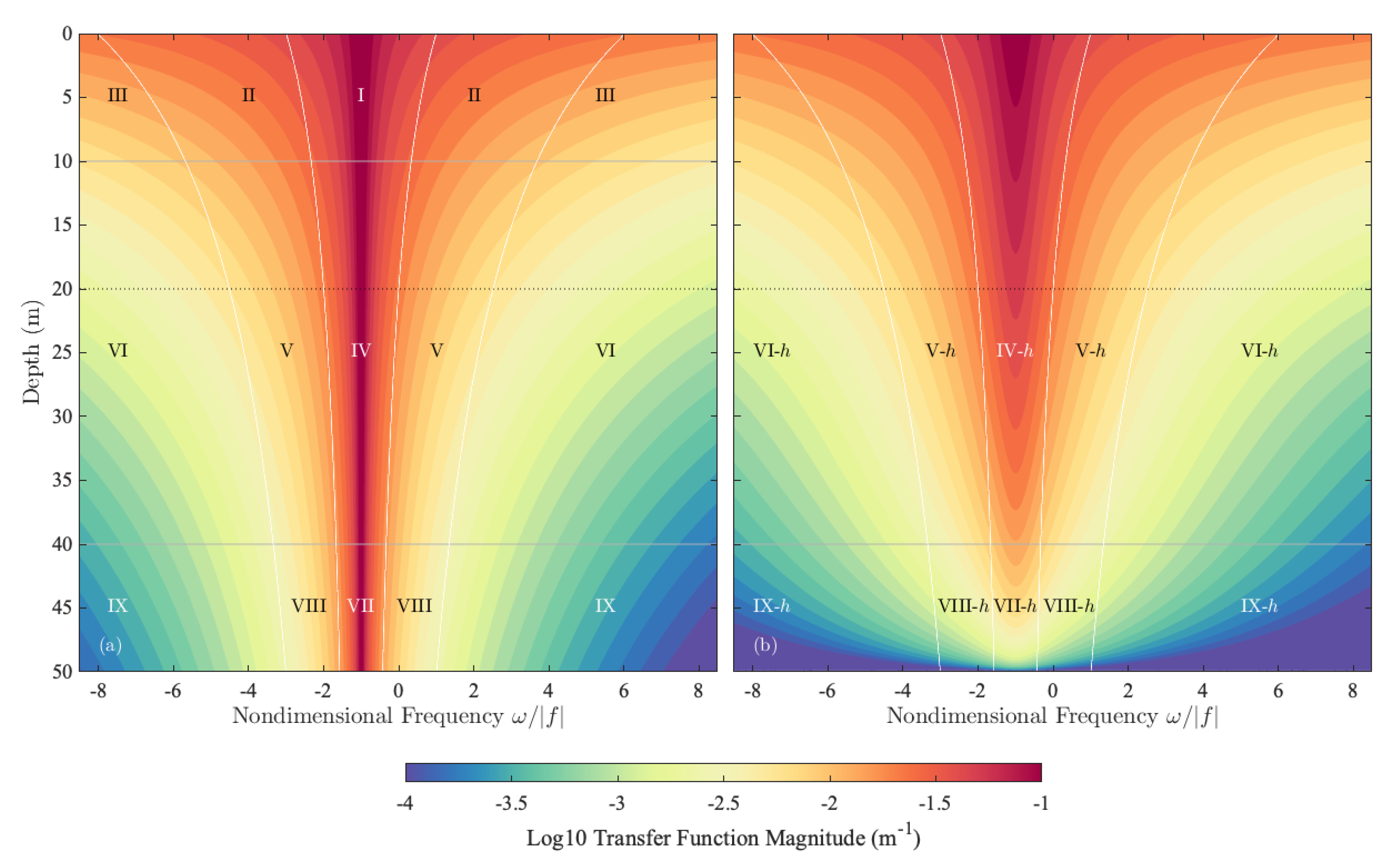
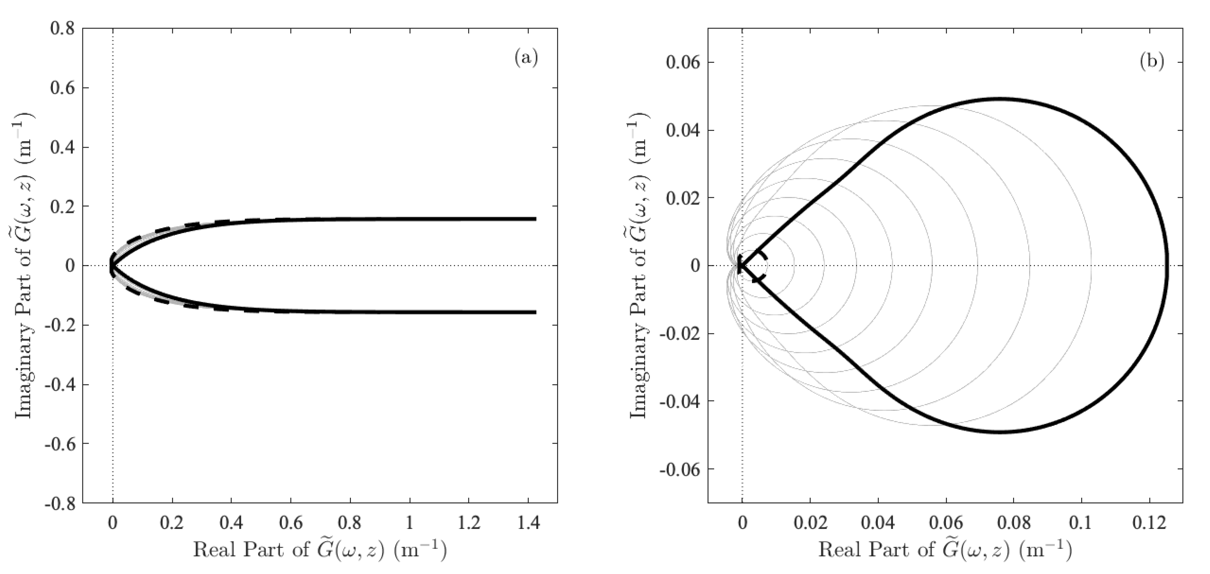
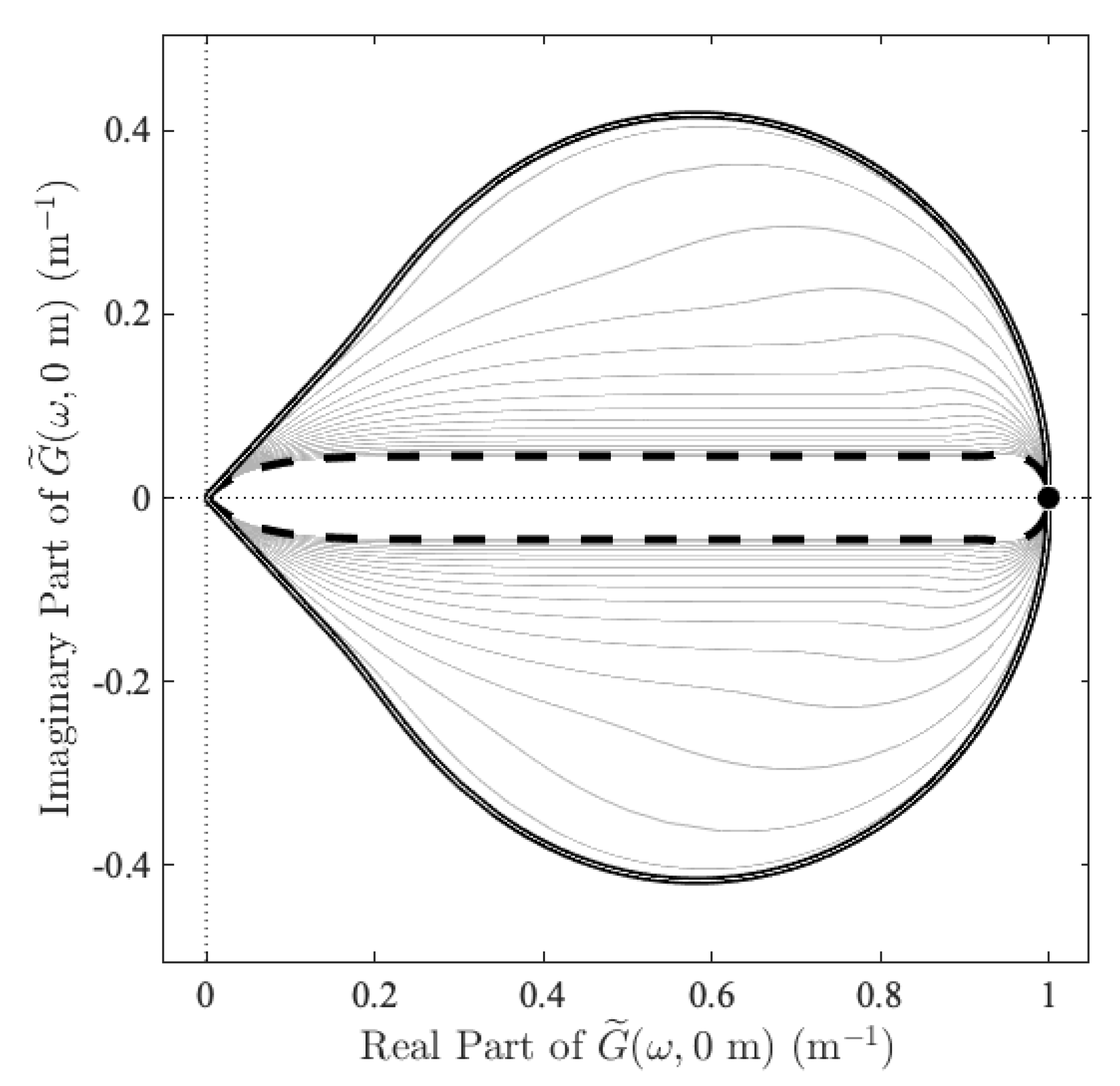
At this point, for orientation, we turn to Figure 1, which presents the dependence of the transfer function amplitude as a function of both depth z and frequency , with the parameter choices m, m, and or m. For these same parameter choices, the curves traced out by the transfer function on the complex plane as varies are shown in Figure 2. Here, as in subsequent figures, we choose , indicating a northern hemisphere location. In both panels of Figure 1, we see a strong maximum centered on the inertial frequency , the Fourier-domain manifestation of the fact that the wind stress forcing excites weakly damped oscillations at that frequency.
Comparing the two panels of Figure 1, we see in both, the transfer function magnitude decays away from the inertial frequency as well as away from the surface. There are two main differences related to the effects of the finite value for h. Whereas for infinite h, the transfer function is unbounded at the inertial frequency—as is most clear from the open curves in Figure 2a—for finite h this singularity becomes smoothed into a finite value. (The importance of the finite depth boundary layer in damping the response to forcing at the inertial frequency can be inferred from the vertically integrated momentum equation, Equation (11), since the left-hand side must vanish for a strictly inertial response.) Because such singularities are not observed in the real ocean, we expect the finite h transfer functions to be more physically meaningful. A second obvious difference is that the rate of decay of the transfer function with increasing depth seen in Figure 1a is heightened in Figure 1b as z approaches the boundary layer depth h, such that the transfer function tends to zero there.
Another feature to note in Figure 2 is the difference in the transfer function curve on the complex plane between the surface and at depth. For , the real part of the transfer function crosses the line , and zooming in reveals that it continually circles the origin as it decays; this occurs for both and m, although it is more apparent in the latter case. This implies that the phase angle of the transfer function is continually increasing or decreasing as the frequency moves away from . By contrast, at the surface, , the two sides of transfer function do not spiral, but rather each approach the origin at a 45 angle to the positive x-axis. Thus, at the surface, there is a 90 phase difference between large positive and large negative frequencies.
3.2. Comparison with the Impulse Response Function
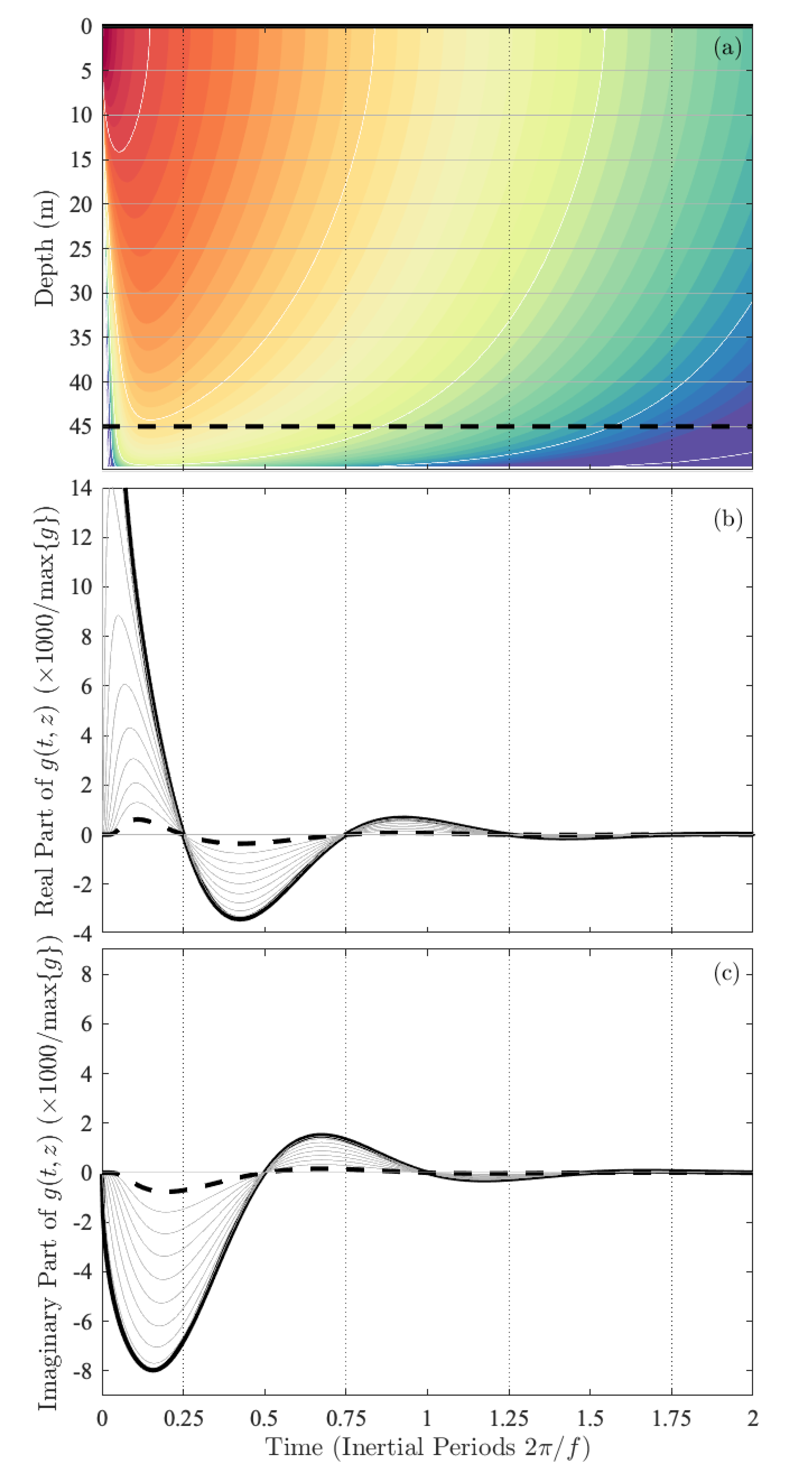
It is useful to compare the finite-depth transfer function shown in Figure 1b and Figure 2b with its impulse response or Green’s function , presented in Figure 3. Because an analytic solution for the full impulse response function is not available, it has been computed numerically as the inverse Fourier transform of . As seen in Figure 3a, the amplitude decays both with time and with depth over most of the domain. For the chosen parameter values, the impulse response function is very rapidly decaying in time, executing little more than a single oscillation before essentially vanishing; this is a consequence of the fact that parameters have been chosen for display purposes in the transfer function schematic of Figure 1. The phase difference between the real and imaginary parts of the transfer function shows a 90 degree offset. When the real part obtains a local maximum, imaginary part will obtain a local minimum a quarter of an inertial period later. This is an expression of the clockwise-rotating circular response expected for inertial oscillations in the northern hemisphere.
At times very close to the origin, rather than decaying, the transfer function exhibits a thin wedge of growing amplitudes that broadens with depth. Very near the surface, the transfer function obtains its maximum value at time , but at deeper depths it rises from an initial value of zero to a maximum amplitude at an intermediate time, leading to an apparent vertical propagation of the maximum response as the momentum of initial impulse is diffused downward from level to level.
3.3. A Second Self-Similarity of the Transfer Function
A second-self similarity of the transfer function allows variations of the Ekman depth, or equivalently of the inertial amplitude, to be absorbed into the frequency axis. To show this we introduce as a frequency deviation that can be used to replace the frequency . Next we define a version of the function, expressed in terms of rather than , as
where we have written the dependence on z as a subscript, as with , and have explicitly indicated the dependence on and . Similarly a new version of the transfer function is defined as
omitting the arguments to on the right-hand side for clarity, and again explicitly indicating the parametric dependencies on the left-hand-side. One finds that and are recovered by
where the right-hand sides can be considered functions of the original parameter set , and h. An important simplification now occurs. For some positive number , one finds
Thus, a rescaling of the Ekman depth can be absorbed into a rescaling of the frequency deviation , together with an amplitude rescaling of the re-parameterized transfer function .
This self-similarity can be framed in an arguably more useful way. The most prominent feature of the transfer function is its value at the inertial frequency, given earlier in Equation (24). We define the amplitude of the rescaled transfer function at the inertial frequency as
The definition of A can be inverted to give as a function of other parameters
and consequently one can replace with A as a controlling parameter. Observe from Equation (31) that multiplying A by is equivalent to multiplying by , which in turn was shown in Equation (29) to be equivalent to multiplying both and by . Thus, as with , the inertial amplitude A can be absorbed into rescaling the frequency deviation together with an amplitude scaling.
The four structural parameters f, (or , , and h have now been reduced to just two parameters determining the transfer function shape, and h, together with two rescalings. The first rescaling absorbs f into the frequency , while the second absorbs the Ekman depth , or equivalently the inertial amplitude A, into the nondimensional frequency deviation , with both rescalings also affecting the overall transfer function amplitude.
3.4. Variability of Transfer Function Structure
The results of the previous section show that in order to investigate the behavior of the transfer function as a function of the four structural parameters f, (or A), , and h, we only need to vary and h. In Figure 4, the rescaled inertial amplitude A, given in Equation (30), is presented for m as a function of and . The depth of observation is chosen as m, as this is the nominal observation depth for surface drifters in NOAA’s Global Drifter Program [42]. The inertial amplitude exhibits a rectangular shape on the vs. plane, decreasing both towards the right-hand side and towards the top of this plot. To understand this shape, we note the asymptotic behaviors
which show that when is small, A decreases with increasing but is independent of for a fixed choice of , while when is large, A decreases with increasing but is independent of . This matches the behavior seen in the plot. The same behavior (not shown) occurs for other choices of h.
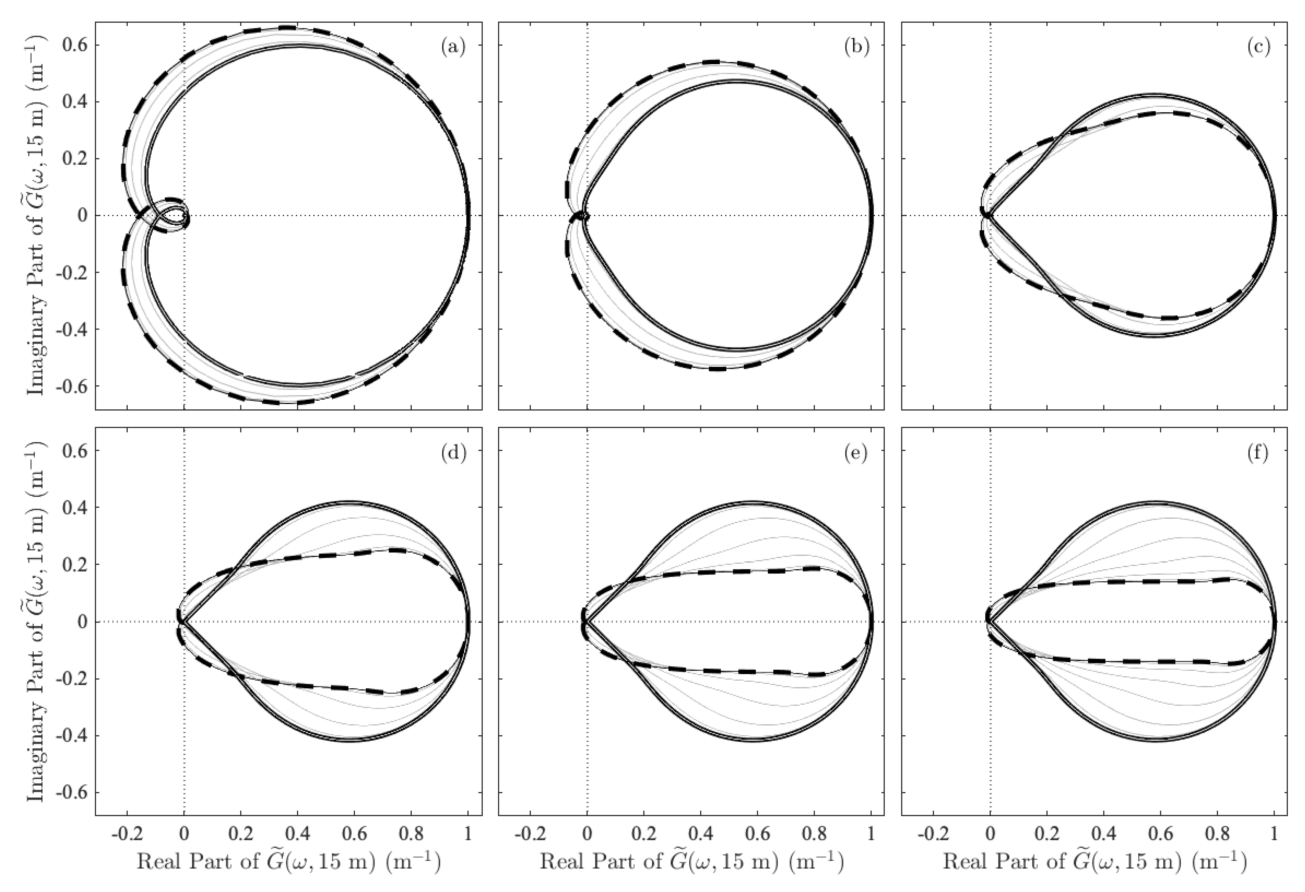
Transfer functions on the complex plane for various values are shown in Figure 5a–f for m, 100 m, 1000 m, 10 m, 10 m, and 10 m respectively; the reason for presenting such large values of h, with a boundary layer depth even exceeding the ocean depth, is to better examine the limiting behavior of the transfer function as h approaches the value of infinity that is implicitly used in the Ekman and Madsen solutions. Other parameter values are chosen such that the inertial amplitude is held fixed at m, while with integer n. For the m case presented in Figure 5c, these values correspond to the black dots shown in Figure 4, a few of which fall beyond the edges of that plot. Because the transfer function shape does not change with and h held fixed, transfer functions that lie along curves of constant in Figure 4 are identical to one another apart from rescaling the amplitude and the frequency axis. Thus, Figure 5c completely characterizes the variability of the transfer function form with the choices m and m, and by examining different h values, Figure 5 essentially captures the entire range of transfer function shapes at m.
We call attention to three features of these transfer functions, explored here graphically, and then in the following section through the asymptotic behavior of the transfer function in various parameter regimes. The first is the overall transition from an Ekman-like solution with to a Madsen-like solution with . In each panel in Figure 5, the transfer function curves transition from the heavy solid line, corresponding to large values or the Ekman-like limit, to the heavy dashed line for small values or the Madsen-like limit. Note that many of the plotted curves are not visible, because near the limiting forms, the curves tend to be extremely similar and lie on top of one another. Comparing panels, we observe that the nature of this transition changes depending on the boundary layer depth h. For panels (a) and (b), corresponding to m and m, the Madsen limit is a broader circle than the Ekman limit, indicating larger transfer function amplitudes. For deeper boundary layer depths h, the situation changes, and the Madsen curve ends up becoming highly elongated along the real axis. Meanwhile, the Ekman curves remain largely circular as h increases, while reducing their radii and shifting their centers towards the positive real direction.
The second feature we call attention to is the phase behavior as the frequency tends to very large positive or negative values. For m, a spiraling of the transfer function around the origin with increasing frequency deviation is clearly seen, meaning that the phase of transfer function continues to increase or decrease as its amplitude decays. As h increases, this spiraling diminishes until it is not longer visible in the plots, however, magnification would reveal that it is still occurring but at smaller amplitudes for larger h values. In general the Madsen-like curves, which all visibly cross the x-axis even for large h, show a greater tendency for spiraling than the Ekman-like curves. This spiraling with increasing frequency deviation is related to the well-known spiraling of the wind-driven currents with depth, as a consequence of the depth/frequency symmetry discussed earlier.
For comparison, the transfer functions for the same parameter settings as in Figure 5c, but for the surface instead of at m, are shown in Figure 6. The transfer functions at the surface have a simpler structure than those at depth, with the versions for other h being qualitatively quite similar to those shown here. A key difference in comparison with the subsurface transfer functions concerns the phase behavior, as spiraling about the origin is not observed at the surface. Instead, the two branches approach the origin at an angle of with respect to the positive x-axis, leading to a 90-degree phase difference between large positive and large negative frequencies. In this plot, the flattening of the transfer function approaching the Madsen-like limit of is even more accentuated than at depth. It will be shown later that the depth-modified transfer function collapses to a single point for all frequencies at in the Madsen-like limit. This is a related to the logarithmic singularity that emerges at the surface in the infinite depth transfer function, and that was noted by [8].
The third feature is the near-inertial behavior, already seen in Figure 1 and Figure 2. As was discussed earlier, a singularity occurs at when the boundary layer depth is set to infinity, but this singularity is damped out for finite choices of h. Thus, one would expect a singularity to begin emerging in Figure 5 as h tends to infinity. The reason it is not seen is that we have specifically chosen parameters in the various panels such that the transfer function amplitude A remains fixed at the value of m, together with the fact that the transfer function curves have been computed on a very dense frequency array. However, with and fixed and h increasing, one would indeed see a singularity emerge, such as was observed between the two panels of Figure 2.
These three features—the transition from an Ekman-like to Madsen-like behavior, shown to be controlled by the phase progression with increasing or decreasing frequency, and the inertial peak, controlled by h—will all revisited in the next section.
4. Asymptotic Behavior of the Transfer Function
In this section we examine the asymptotic behaviors of the general no-slip transfer function , given by Equation (23), for various limits of its controlling parameters, unifying the results from a number of earlier studies.
4.1. Regimes of the Transfer Function
In investigating limiting behaviors, , , and emerge as controlling quantities, all three of which may be larger than, equal to, or smaller than one. The ratio determines whether the gradient of the vertical viscosity is strong or weak. When the gradient is strong, the roughness length is small compared with , and the dynamics are Madsen-like—by which we mean dominated by —while when the gradient is weak, the dynamics are Ekman-like or dominated by . The ratio controls the nondimensional position of the observation depth. Finally, determines the extent to which the solution is influenced by the effect of a finite-depth boundary layer.
At this point a new notation will be introduced to help keep track of the ordering of parameters in various limits:
The symbol “” is an arrow superposed on a less than sign, indicating an ordering as well as a limit; the notation “” is not sufficient because it simply means that a is much less than b, as opposed to the limit as tends to zero that is required here. An advantage of this approach is that we can order multiple variables, such that
with the former being a more compact and legible notation.
4.2. Transfer Function Expressions
Asymptotic forms of the general no-slip transfer function are presented in Table 1, for the limit of large h, and Table 2 including the effects of finite h. Each table is a matrix in which the three columns are for the three possible relationships between and (, indeterminate, and with , respectively), while the three rows are for the three possible relationships between z and (, indeterminate, and ). The orderings implied by the intersections of the row limits and the column limits are detailed in each entry of the tables. In addition to , given earlier in Equation (20), two related functions,
emerge in the limits of small or large nondimensional observation depth , respectively.

Table 1.
Parameter space behavior of the general no-slip transfer function in the limit of large boundary layer depth h as a function of the ratio and ratio, numbered I–IX. Here and are decaying modified Bessel functions of order of the first and second kind, respectively, the Madsen depth is regarded as a function of the Ekman depth and roughness length , and is a sign function. The functions , , and are three different versions of the arguments to the Bessel functions that appear in the upper, middle, and lower rows, respectively; note . The boxed terms were previously presented by Elipot and Gille [12], with “EG” refers to the numbering nomenclature of those authors. The transfer functions for the Ekman [4] solution and Madsen [8] solutions are in the upper right-hand corner and lower left-hand corners.
| Strong Gradient/Near-Inertial | Arbitrary Gradient/Any Frequency | Weak Gradient/Far-Inertial | |
|---|---|---|---|
| or | — | ( and ) or | |
| I | II | III, Ekman, EG-1a | |
| ∞ | |||
| IV | V, Mixed, EG-3a | VI | |
| VII, Madsen, EG-2a | VIII | IX | |
| 0 |
Table 2.
As with Table 1, the parameter space behavior of the general no-slip transfer function , but now including the effects of the finite boundary layer depth h and numbered I-h–IX-h. Again the functions , , and are versions of the arguments to the Bessel functions appearing in the upper, middle, and lower rows. As before, is regarded as a function of and , and is a sign function. The boxed terms were previously presented by Elipot and Gille [12]. Note that in all regimes, but only in the upper row, where , is there a required assumption for the size of h versus the other parameters.
| Strong Gradient/Near-Inertial | Arbitrary Gradient/Any Frequency | Weak Gradient/Far-Inertial | |
|---|---|---|---|
| or | — | ( and ) or | |
| I-h | II-h | III-h, Depth-modified Ekman, EG-1b | |
| IV-h | V-h, Depth-modified mixed, EG-3b | VI-h | |
| — | |||
| VII-h, Depth-modified Madsen, EG-2b | VIII-h | IX-h | |
The infinite h regimes in Table 1 are denoted by Roman numerals I–IX, while the finite h regimes in Table 2 are denoted by I-h, II-h, etc. All forms in these tables can be derived under the indicated limits from the general solution presented earlier in Equation (23), for and finite h, which inhabits regime V-h at the center of Table 2. When limits of both and are involved, these may be taken in either order. For example, in moving from V-h to VII-h, one may move first left and then down or first down and then left. All of the infinite h forms in Table 1 can be derived by first deriving form V from V-h, then taking appropriate limits of and of , or alternatively by taking the infinite h limit of the corresponding expression in Table 2, yielding identical results in either case. Relevant details on the derivations of the asymptotic forms are given in Appendix F.
All six terms along the two anti-diagonals—those enclosed in boxes—were previously presented by Elipot and Gille [12], and are labeled according to the numbering system of those authors, e.g., EG-1a, etc. (Note that in [12], is occasionally rewritten as , which is not correct; this applies to transfer functions 1a, 1b, and 1c in the first row of their Table 1. While , changing the sign inside the radical gives which is not the same as .) These were derived therein as six separate cases, by setting , , or in the transfer function equation, Equation (13), and then setting a lower boundary condition of velocity vanishing at either an infinite depth or at . All of the other forms in these tables are new. The new expressions are useful as giving the intermediate steps in the derivations that move from the central form to the upper right and lower left asymptotic limits, and are also themselves relevant approximations to the transfer function under certain dynamical regimes.
The expressions in these tables either explicitly or implicitly subsume the results from a number of earlier studies, as we will now discuss in detail, clarifying a point made by Elipot and Gille [12]. Form III is the transfer function for the Ekman case () with currents vanishing at infinity, first presented by Gonella [6] following the derivation of the associated impulse response function by the same author [5]. The impulse response function corresponding to form III is, in turn, closely related to the switch-on solution given in Ekman [4] and attributed to I. Fredholm. As discussed in Section 2.1, the solution to the switch-on problem in the frequency domain can be readily expressed in terms of the transfer function as . Similarly, frequency-domain versions of the switch-on solutions derived by Lewis and Belcher [11] for the general linear viscosity profile for infinite depth, and for or for both infinite and finite h values, are readily found from forms V, III, III-h, VII, and VII-h. Considering the Ekman problem modified for the effects of finite depth, Krauss [7] found the impulse response function as well as its Laplace transform, the being essentially identical to the transfer function in III-h apart from a change of variables. Finally, the transfer function in regime VII is basically the same as the Laplace transform solution of Madsen [8].
4.3. Survey of Asymptotic Behavior
Next we survey the behaviors in Table 1 and Table 2, with reference to the Ekman/Madsen transition, the spiraling behavior with increasing frequency discussed earlier, and the near-inertial peak.
The Ekman-like () and Madsen-like () solutions—in the upper-right hand and lower-left hand corners of these tables, respectively—are seen to represent opposing limits around which the behavior of the transfer function can be characterized. The right-hand columns of both tables can be thought of as “near-Ekman”, or close to the behavior but with a minor effect due to the vertical gradient of viscosity. Similarly, the left-hand columns can be thought of as “near-Madsen”, or close to the behavior but with a minor effect due to the surface value of the viscosity. The transitions to pure Ekman or Madsen dynamics, in which the effect of or , respectively, is entirely neglected, is seen to involve not only a condition on the regime parameter but also on the nondimensional depth . An interesting aspect is how the Ekman and Madsen solutions interact. The Ekman-like solutions in regimes III and III-h contain no dependence on or on , while the Madsen-like solutions in regimes VII and VII-h contain no dependence on . For all other forms, both and , or else and , are required. In other words, all other entries apart from the lower left and upper right corners are mixed in the sense that they include to some extent the influence of both the surface value of the viscosity as well as its gradient . The more general expressions in the central column are required when strengths of these two effects are roughly comparable.
One interesting aspect of the Ekman/Madsen transition concerns the surface singularity of the Madsen solution. The original Madsen solution in regime VII has a logarithmic singularity at , a consequence of the asymptotic behavior for . As was pointed out by Madsen [8], this is an unrealistic aspect of that solution. (The effect of a finite depth does not help, since form VII-h still has the surface singularity, due to the fact that as we have for all fixed frequencies.) This problem lead Lewis and Belcher [11] to consider the offset linear eddy viscosity , for which they derived a switch-on solution for the infinite depth case, comparable to our regime V. However, the “near-Madsen” solutions in regimes IV and IV-h, in which the role of is small but non-negligible, also have this singularity removed, showing that only a small value of the eddy viscosity at the surface is sufficient to resolve this unphysical feature.
Regarding the phase behavior at large positive and negative frequencies, we see from the Ekman transfer function, form III, that for , the phase of the transfer function is given by . This implies that between very large positive and very large negative frequencies, the change in phase of the transfer function will be , or 90 degrees. The same behavior can be found by taking the large frequency deviation limit of the general form V-h. This 90-degree phase difference at is a thus general results for all parameter choices, apart from the pure Madsen solution which is singular at the surface. This explains the pattern seen earlier in Figure 6. For , numerical computation shows the phase to increase or decrease continuously as one proceeds to large frequency deviations , leading to the spiraling behavior seen in Figure 5.
The value of the transfer function at the inertial frequency , previously presented in Equation (24), holds for all parameter values and is most readily derived from the near-Madsen forms in the left-hand columns of these tables. When h is infinite, the value of the transfer function at the inertial frequency is unbounded, leading to the well-known singular behavior seen earlier in Figure 2a. The singularity is removed with the introduction of a finite boundary layer depth h, as seen in Figure 2b. As such singularities are not observed in reality, all of the infinite h transfer functions considered here have a prominent feature that is physically unrealistic.
4.4. A Depth/Frequency Interpretation of Regimes
The asymptotic behaviors seen in Table 1 and Table 2 not only give limiting forms appropriate for various parameter choices of different transfer functions, but also, to an extent, those occurring at different frequencies or depths within the same transfer function. The columns of Table 1 and Table 2, which set the regime of the ratio, can alternatively be seen as specifying the regime of the frequency deviation . The ratio acts through the function, given in Equation (20), that appears in the arguments to the Bessel functions, and limiting behaviors occur when those arguments are either very small or very large. The limit is thus essentially equivalent to , while with is essentially equivalent to . For this reason, , and with , may be referred to as the near-inertial and far-inertial limits, respectively.
In the case of Table 1, we may therefore see these expressions as asymptotic forms arising on the depth / frequency, or , plane for any individual realization of the transfer function, provided and are both nonzero. In other words, one expects to see these regimes approximately occurring within a given transfer function, as labeled in the schematic in Figure 1a, not only between transfer functions with different parameters. Thus, the classical Ekman solution is the asymptotic behavior of the general no-slip transfer function with in its near-surface, high-frequency limit, while the Madsen solution arises in the deep, near-inertial limit. For Table 2, the interpretation of the rows as pertaining to depth regimes within a given transfer function no longer applies, because the upper and lower rows involve opposing limits of the ratio . For the upper row is suitable for all z, whereas for the lower row becomes suitable for sufficiently large z, as indicated in Figure 1b.
The depth/frequency interpretation of transfer function regimes may not be practically useful, because a transfer function is generally needed for all resolved frequencies, not just for a particular depth and frequency range. Nevertheless, it is helpful to conceptually organize the different regimes in terms of where they occur on the depth/frequency plane.
4.5. Impulse Response Functions
Of all the transfer function forms listed in Table 1 and Table 2, only a few appear to have corresponding analytic expressions for the impulse response function: form III, due to Gonella [5,6]; form VII, due to Madsen [8]; form IV, which will have an analytic solution that is very similar to that for form VII; and the depth-modified Ekman solution in III-h, the impulse response function for which was shown by Krauss [7] to involve a Jacobi theta function. Here we will present the impulse response functions only for the Ekman and Madsen solutions, which are found to be, respectively,
with again being the unit step function. These impulse response functions correspond, respectively, to the transfer functions
which have been rewritten from Table 1 for easier comparison.
When the wind stress forcing consists of a Dirac delta function in time, , then from Equation (1) the current response is simply the impulse response function . It is straightforward to verify that and are in fact valid solutions for an impulsive forcing with . That the time-domain momentum equation, Equation (8), is satisfied can be readily shown by differentiating and . The upper boundary condition is then best examined through the vertically integrated momentum equation, Equation (11), with h set to a value of infinity. Noting first that , differentiation shows that
for both and , using the fact that . This matches the right-hand-side of Equation (11) emerging from the upper boundary condition for . The lower boundary condition of vanishing flow at infinite depths is clearly satisfied.
While and have both been verified to be solutions to the relevant equations of motion, establishing that they are a Fourier transform pair is more difficult due to a subtlety involving the relevant integral formula. The same is true for and . In Appendix G, we show that and , and similarly and , are in fact Fourier transform pairs in the limit that an artificially introduced damping parameter tends to zero.
These two impulse response functions possess a similar structure. In addition to rotating on the complex plane in the anticyclonic sense at frequency , both functions are zero for negative times and decay for both large times and large depths. For , both impulse response functions rise to obtain a maximum modulus at intermediate times that grows with increasing depth, since differentiating shows that is maximized at time while is maximized at time . The decay of the Madsen’s impulse response function for large times is somewhat faster on account of an additional in the denominator, which also makes the initial growth to the maximum somewhat slower. The depth scale is controlled by for the Ekman case and for the Madsen case, as expected. The former decays more rapidly with nondimensional depth on account of the appearing in the exponential, compared with the linear decay in the latter case. Qualitatively these behaviors match those for the numerically computed transfer function presented earlier in Figure 3.
5. Discussion
This paper has examined the unsteady response of the near-surface ocean currents to a surface wind stress, what we refer to as the unsteady Ekman problem. The frequency-domain solution for a general linear eddy viscosity profile with currents vanishing at the bottom of a boundary layer of a finite depth h was considered. It was shown that the fundamental quantity involved in the frequency-domain solution, the transfer function, allows the solution for general wind forcing to be readily expressed, and also encompasses the solutions to related problems such as the switch-on problem and the steady response. This general linear transfer function, first derived by Elipot and Gille [12], was shown to include as asymptotic limits five other transfer functions derived by those authors as special cases, thereby unifying the results of numerous earlier studies including Ekman [4], Krauss [7], Madsen [8], and Lewis and Belcher [11], and amounting to the most general expression for the transfer function yet produced. This unification is the main result of the paper. As discussed in the Introduction, establishing a nested family of transfer function forms is an important prerequisite to being able to determine which range of parameters provides the best fit against observations, and thus improve predictions of the near-surface velocity given the winds.
Examining the dependence of the transfer function on its parameters, we showed how taking two self-similarities into account allows one to more clearly see the range of its possible forms. The roughness length emerged as the primary parameter controlling the transfer function shape for a fixed boundary layer depth h, while the choice of boundary layer depth h was seen to determine the strength of the inertial peak, which becomes singular as h tends to infinity. A numerical issue was uncovered that prevents the evaluation of the transfer function from leading to sensible results, a problem that was solved in Appendix E through the use of series expansions for the Bessel functions.
As mentioned in the Introduction, it is important to assess the potential relevance of this work within the context of our understanding of physics of the real ocean. Here an important issue is whether observation depths are sufficiently shallow compared to the Ekman depth such that the eddy viscosity profile might be well approximated by a linear function. To address this, we first we review some published estimates of the Ekman depth, denoted herein. Estimates based on in situ observations are not common, but previous works have placed it at 25 or 48 m using two different estimation methods in a study of the California Current [49], 22 or 59 m using two different estimation methods in a study of the Drake Passage based on repeated observations [50], and 39 m [51] in a reanalysis of the Drake Passage data; the review in Section 6.3.4.1 of Rio and Hernandez [52] quotes several other studies giving comparable values. Global estimates are rarer still, but in an application of a parametric model for the steady wind-driven response using current observations from the global drifter dataset, Rio and Hernandez [52] obtain estimates of the Ekman depth (deduced from the parameters of their model) of 30–60 m in the summer hemisphere, and 60–120 m in the winter hemisphere apart from in subpolar southern latitudes where smaller values of 0–50 m were observed.
These estimates of Ekman depth can be connected to the expected vertical profile of the eddy viscosity by appealing to the large eddy simulation study of Zikanov et al. [20]. While those authors do not explicitly state the Ekman depth that best fits their simulations, a visual examination of their Figure 4b shows that their Ekman profile has its e-folding depth—corresponding to our —at about 0.2 of their nondimensional units below the surface, roughly the same depth at which their inferred eddy viscosity profile, in their Figure 5d, obtains its maximum. Thus, based on the results of this numerical study, we would expect the eddy viscosity to obtain its maximum at a depth comparable to the Ekman depth. Consequently, the eddy viscosity at depths smaller than the Ekman depth should be reasonably well approximated by a linearly increasing profile. In comparison with the values quoted in the previous paragraph, we conclude that the 15 m observation depth of the global drifter dataset should be well within this linearly increasing range over much of the ocean. A question mark, however, is the physical realism of setting the flow to vanish at the base of a boundary layer at which the eddy viscosity has its maximum, and whether this may lead to differences in the transfer function compared with the linearly increasing regime of a viscosity profile having an intermediate maximum. Understanding the relevance and limitations of the linear viscosity profile is a promising topic for future work.
Recently, several important papers have examined the near-surface currents under the assumption of more realistic or more general eddy viscosity profiles. Shrira and Almelah [15] examined the unsteady Ekman problem for a more general eddy viscosity profile than that employed here, equivalent to in our notation for some power , and with and having the potential to be functions of time. Solutions were found for currents vanishing at an infinite depth. For the case, using a different transformation from that employed here, those authors obtain an equivalent Bessel function equation in the Laplace transform domain to our Equation (13), see their Equation (3.13). The close similarity between their expressions and ours suggests that it should be straightforward to modify their results to account for the effect of a finite boundary layer depth h, thus encompassing a broader range of solutions. Whether these more general solutions could be written in the form of a transfer function is not immediately clear owing to the complicated transformations involved.
As mentioned in the Introduction, an expression that is essentially the transfer function solution for the Ekman problem with a cubic eddy viscosity profile proportional to was found by Song and Xu [14]. Inspired by their results, one may consider the quadratic eddy viscosity profile
with . This eddy viscosity has the advantage of a realistic form that increases and then decreases again, while also subsuming all of the previously considered constant and linear solutions, which the cubic profile proportional to does not accomplish. Re-deriving our Equation (13) for the transfer function but for the quadratic viscosity profile, and with the substitutions (see p. 239 of Ref. [53])
one obtains Euler’s hypergeometric equation for the transfer function
the solutions of which, like those for the cubic profile in Song and Xu [14], are known in terms of the Gaussian hypergeometric function . The examination of the solutions for the quadratic family of eddy viscosity profiles would be another important step towards a unified solution of the unsteady Ekman problem. It is also possible that the solution of Song and Xu [14] could be extended to a more general cubic form, if desired.
An area of active research is understanding the role of Stokes drift and wave breaking in modifying the near-surface wind-driven currents [11,14,15,17,18,19]. These effects have in fact already been incorporated into the linear eddy viscosity model by Shrira and Almelah [15], though those authors work in the Laplace rather than the Fourier domain. As discussed in Appendix B therein, the Ekman problem with a general linear viscosity profile is modified by the presence of a Stokes drift, to lowest order, through a forcing term appearing in the momentum equation, our Equation (8). The solution then consists of the general solution to the homogeneous problem together with a particular solution to the inhomogeneous problem, itself expressible as an integral of the forcing against solutions to the homogeneous problem. Thus, the transfer function solution is simply augmented with an integral over the Stokes drift, assuming that the latter is known. The work of Song and Xu [14] to incorporate Stokes drift as well as wave-induced momentum deposition into the Ekman problem, in the context of the cubic profile proportional to , is quite closely related to that of Shrira and Almelah [15]. This suggests that by following the work of those authors, Stokes drift and wave momentum deposition could also be incorporated into the general quadratic eddy viscosity profile proposed in the previous paragraph.
Finally, several relevant recent studies have investigated solutions to the steady Ekman problem. In a simplifying work, Dritschel et al. [16] find analytic solutions to the steady Ekman spiral for a piecewise linear eddy viscosity profile. Similarly, Ionescu-Kruse [41] finds steady solutions for power-law eddy viscosities proportional to or , while Bressan and Constantin [54] and Constantin [55] solve for the steady Ekman currents for an eddy viscosity profile that consists of a depth-dependent perturbation about a constant value. It is possible that results of those works could be fruitfully brought to bear on the unsteady problem considered here.
6. Materials and Methods
Numerical code relevant to this paper is released as a part of a freely-available open-source toolbox for Matlab maintained by the first author. The toolbox, called jLab, is available for download from https://github.com/jonathanlilly/jLab with installation instructions and detailed online documentation available at http://www.jmlilly.net/software.html. The primary function related to this paper is called windtrans. This implements the general no-slip transfer function of Equation (23), as well all of the boxed forms in Table 1 and Table 2. The default formulation uses the tilde-function approach developed in Appendix E to avoid numerical overflow. All figures are created with the script makefigs_transfer.
Author Contributions
Conceptualization, S.E. and J.M.L.; formal analysis, J.M.L.; software, J.M.L.; investigation, S.E. and J.M.L.; visualization, J.M.L.; writing—original draft preparation, J.M.L.; writing—review and editing, J.M.L. and S.E.; project administration, S.E. and J.M.L.; funding acquisition, J.M.L. and S.E. All authors have read and agreed to the published version of the manuscript.
Funding
The work of J.M.L. was supported by awards #1459347 and #1658564, and that of S.E. by award #1459482, from the Physical Oceanography program of the United States National Science Foundation. The authors extend their thanks to two anonymous reviewers, whose comments and questions led to an improved manuscript.
Conflicts of Interest
The authors declare no conflict of interest.
Appendix A. The Transfer Function Relation
In this appendix we show that the wind-driven currents can be expressed through the Fourier domain form presented in Equation (5). Firstly we rewrite the spectral representation for , Equation (2), bringing the mean wind stress inside the integral to yield
and we similarly rewrite the spectral representation for . Then substituting these, together with expressed in terms of its Fourier transform as in Equation (4), into Equation (1), we obtain
after making use of . This reduces to Equation (5) as claimed.
Appendix B. Derivation of the Modified Bessel’s Equation
In this appendix we derive the modified Bessel’s equation for the transfer function given in Equation (21). To do this we first rewrite Equation (13) for in terms of and as
and then observe that the first two z-derivatives of satisfy
Applying the change of variable relations
one obtains Equation (21) after a few lines of algebra.
Appendix C. Verification of the Boundary Conditions
In this appendix we verify that the general no-slip transfer function given in Equation (23) does indeed satisfy the specified boundary conditions. For notational convenience, we let and in this and following appendices, with the superscript denoting the z-argument of inside the Bessel functions. Using this notation, Equation (23) becomes
where we have also noted that . To verify the upper boundary condition, Equation (14), we compute the partial derivative with respect to depth,
in which we have made use of Equation (9.6.27) of Abramowitz and Stegun [46] for the derivatives of the zeroth-order Bessel functions, namely
The z-derivative of is found from Equation (18) to be
Evaluated at , the ratio of Bessel functions in Equation (A9) becomes unity, and the vertical derivative of the transfer function evaluated at the surface thus becomes
as required for the upper boundary condition. It is clear from inspection of Equation (A8) that vanishes, satisfying the lower boundary condition.
Appendix D. The Free-Slip Transfer Function
The transfer function with a linearly varying eddy viscosity, , and a free-slip lower boundary condition at the bottom of the boundary layer, , is
which corrects a typographic error in Elipot and Gille [12]. This has the form given in Equation (22) and therefore satisfies the differential equation for in Equation (21). Its first z-derivative is
which vanishes at and reduces to Equation (A12) at , thus satisfying both boundary conditions. The near-inertial asymptotic behavior of the free-slip transfer function is found to be
which contrasts with Equation (24) for the no-slip case; note that this behavior is independent of the choice of or , and therefore occurs whether or not there is a gradient of the vertical viscosity. In addition to a singularity at , the free-slip transfer function exhibits a 90-degree discontinuous phase jump across the inertial frequency on account of the sign function . This is in opposition to the observations, which show a phase that smoothly approaches zero near the inertial frequency [12]. Thus, this transfer function does not appear to be realistic, and it need not be investigated any further.
Appendix E. Numerical Computation of the Transfer Function
In this appendix a difficulty in computing the transfer function, Equation (23), arising from numerical overflow is identified and solved. The problem is illustrated in Figure A1a. With m, the transfer function is computed at frequency and depth m over a broad range of parameter space on the vs. plane. The transfer function evaluation fails around the location of the gray line, which marks the location where for . Below this line, some terms in Equation (23) exceed the largest representable number in double-precision format, about .
This numerical overflow arises as consequence of the exponential behavior of the modified Bessel functions for large arguments, see Equations (9.7.1) and (9.7.2) of Abramowitz and Stegun [46],
and may be traced to two different sources. The first problem occurs if one lets h become large with the ratio held fixed, while considering a fixed depth z and a fixed off-inertial frequency . Examining the form of in Equation (20), we see that as h becomes large, the magnitude of becomes large while or remain fixed. The problem of large is handled simply by rewriting the Bessel function ratio in Equation (23) as
using and for notational convenience. Now, as becomes large, rather than causing numerical overflow from the exponentially growing Bessel functions, the terms in the parentheses in the numerator and denominator of Equation (A18) will tend to zero. Then as h increases, the transfer function will smoothly approach the form for an infinitely deep layer, as presented in regime V of Table 1.
Figure A1.
An illustration of overflow problems in computing the transfer function, and their solution. The transfer function at frequency and depth m is computed on the vs. plane with m using (a) Equation (23) directly or (b) using the tilde-function formation of Equation (A20) for Bessel function ratio. In the latter case, 30 terms are used to compute and via Equations (A21) and (A22). The same color scale is used in both (a,b). Panel (c) is a comparison of the asymptotic or one-term expansions of Equations (A16) and (A17) versus the 30-term expansions. The quantity shown in panel (c) is the fractional error, defined as the magnitude of the asymptotic version minus the 30-term version, all divided by the 30-term version. The gray diagonal line marks the location on the vs. plane where , and is the location where begins to overflow.

The second problem occurs as the ratio becomes large with other parameters held fixed. As this ratio increases, the magnitudes of , , and all become large provided . To overcome this problem, we define variants of the Bessel functions that have the leading exponential dependence explicitly removed,
The Bessel function ratio in Equation (23) then becomes, with and ,
after rearranging the exponential terms to prevent overflow from large discussed previously. In this form, the exponential growth from the modified Bessel functions of the first kind , and the decay from the modified Bessel functions of the second kind , are arranged to partly cancel.
The and functions can then be expanded as the power series. With being a small number, these have the expansions
provided that the indicated phase conditions are satisfied, which is the case here as the arguments of the Bessel functions will have . The coefficient is defined as
The series expansions in Equations (A21) and (A22) are given in Equations (9.7.1) and (9.7.2) of Abramowitz and Stegun [46], or more explicitly in Equations (10.40.1) and (10.40.2) of NIST [56]. Note that the first term in both series is unity, in agreement with the asymptotic behaviors in Equations (A16) and (A17).
The accuracy of these approximations for complex-valued arguments like those occurring in the transfer function is assessed as follows. For a fixed number of terms, we compute with real-valued x using Equation (A21) and as using Matlab’s built-in besseli function. The latter will be taken as the true value. Using 30 terms in Equation (A21), the approximation minus the true value, all divided by the true value, has a magnitude less than with and for or 1. The same applies for in Equation (22) compared with besselk with . Thus, these series offer a high degree of numerical precision after 30 terms for even relatively small values of the argument. Because the and functions can be represented accurately, while the exponential growth terms have been arranged to cancel, we can now evaluate the transfer function for large values of with very high accuracy.
Employing this tilde-function approach to computing the Bessel function ratio in the transfer function, as in Equation (A20), is an order of magnitude slower than directly calling besseli and besselk, and therefore we do not wish to use it for all parameter values. However, as the overflow due to large is already handled simply by rewriting the Bessel function ratio as in Equation (A18), the tilde-function approach only need be used when the second-largest Bessel function argument, , also leads to overflow. In implementation, we switch to computing the Bessel function ratio using Equation (A20) whenever the magnitude of exceeds , a threshold that is slightly below where begins to overflow. In Figure A1b, the computation of the transfer function with the same parameter values as in panel (a) is accomplished by switching to the tilde-function version in this way. The transfer function can now be accurately computed over a wide parameter space.
By contrast, simply using the asymptotic behaviors in Equations (A16) and (A17) instead of the power series in Equation (A21) and (A22) offers unsatisfactory performance. Figure A1c shows that the difference between the asymptotic or one-term expansion and the 30-term expansion is non-negligible, with the fractional error approaching over much of the domain. This error is largest at the location where the algorithm switch is implemented. Recall that one goal of this work is to be able to use the transfer function in an optimization scheme to identify the parameters giving currents that best match the observations. Such optimizations are highly sensitive to the texture of the optimization function, such that discontinuity seen in Figure A1c would be expected to lead to an obvious numerical artifact.
Appendix F. Derivation of the Asymptotic Forms
In this appendix we discuss the derivation of the asymptotic expressions in Table 1 and Table 2. Firstly, we note that when taking a limit such as , the other parameters are considered indeterminate rather than fixed. Thus, for example, if we take , this does not mean that the product tends to zero, because we may later consider the opposing limit .
The derivation of the asymptotic expressions is primarily a matter of applying the asymptotic properties of the modified Bessel functions for large arguments, Equations (A16) and (A17), together with those for small arguments,
see Equations (9.6.7)—(9.6.9) of Abramowitz and Stegun [46]. We have also made use of the Taylor series
as well as the relations
The latter, which combine the subtraction formulas for hyperbolic functions with their definitions in terms of exponentials, are used in moving from the central column of Table 2 to the right-hand column.
A relatively subtle case arises in moving from the central finite depth column, regimes II-h, V-h, and VIII-h, to the left column. In the case of V-h, applying the limit gives
for the denominator of the Bessel function ratio, using Equations (A24) and (A25) for the quantities containing . Since implies , it would seem that the second term in square brackets is negligible relative to the first; however we should also consider possible asymptotic behavior of . In the large argument limit, as occurs for , we see that is negligible relative to . If instead h is considered fixed, then we have for that
again using Equations (A24) and (A25). The second term on the right-hand side is of the form , which vanishes in the limit of small x by l’Hôpital’s rule because
Thus regardless of whether h is fixed or tending to infinity, we have for that
and using this, we obtain IV-h from V-h. The same argument gives I-h from II-h and VII-h from VIII-h.
To derive the Ekman and depth-modified Ekman solutions, presented in forms III and III-h respectively, as limits of more general expressions in the central columns, the inertial frequency must be considered separately. This is because the asymptotic behaviors based on the limit , used in moving from the central column of each table to the right-hand column, do not hold at exactly the inertial frequency. Nevertheless, forms III and III-h do indeed have the correct behaviors at , as can readily be verified. At , the depth-modified Ekman transfer function III-h reduces to I-h, as is shown with the help of the asymptotic behaviors and for . This matches the behavior of the more general form II-h at , and is the same as the behavior of the full transfer function V-h at , given by Equation (24), in the limit . Considering form III, the non-depth-modified Ekman solution, we see that it is, correctly, unbounded at the inertial frequency. Thus forms III and III-h do give the correct behaviors at the inertial frequency.
Appendix G. The Ekman and Madsen Impulse Response Functions
In this appendix it is shown that the Ekman and Madsen impulse response functions, and in Equations (38) and (39) respectively, are, in a certain limiting sense, the inverse Fourier transforms of the corresponding transfer functions and from Equations (40) and (41). For the Ekman case, we begin with Equation (3.471.15) of Gradshteyn and Ryzhik [57]
which becomes, choosing for real-valued and with ,
Next we define a modified version of the Ekman infinite-depth transfer function from Equation (40)
which has as its inverse Fourier transform
as follows from Equation (A33) with set to . Here plays the role of a damping which is necessary only to ensure the validity of the integral relating and . Letting this quantity become infinitesimally small, we define , and obtain Equation (38).
For the Madsen impulse response function, Equation (10.32.10) of NIST [56] gives, for the case of the Bessel function of order , the integral representation
the history of which is discussed in Watson [58] (p. 183). With the substitutions and for real-valued , , and , and with and , this becomes
As before we define a modified version Madsen transfer function from Equation (41) as
which has as its inverse Fourier transform, setting in Equation (A37),
and again taking the limit as the damping parameter tends to zero, we obtain Equation (39).
References
- Watanabe, M.; Hibiya, T. Global estimates of the wind-induced energy flux to inertial motions in the surface mixed layer. Geophys. Res. Lett. 2002, 29, 1239. [Google Scholar] [CrossRef]
- Wunsch, C.; Ferrari, R. Vertical mixing, energy, and the general circulation of the oceans. Annu. Rev. Fluid Mech. 2004, 36, 281–314. [Google Scholar] [CrossRef] [Green Version]
- Zhai, X.; Greatbatch, R.J.; Eden, C.; Hibiya, T. On the loss of wind-induced near-inertial energy to turbulent mixing in the upper ocean. J. Phys. Oceanogr. 2009, 39, 3040–3045. [Google Scholar] [CrossRef]
- Ekman, V.W. On the influence of the Earth’s rotation on ocean currents. Ark. Mat. Astr. Fys 1905, 2, 1–36. [Google Scholar]
- Gonella, J. A local study of inertial oscillations in the upper layer of the ocean. Deep-Sea Res. 1971, 18, 775–788. [Google Scholar] [CrossRef]
- Gonella, J. A rotary-component method for analyzing meteorological and oceanographic vector time series. Deep-Sea Res. 1972, 19, 833–846. [Google Scholar] [CrossRef]
- Krauss, W. Wind-generated internal waves and inertial-period motions. Dtsch. Hydrogr. Z. 1972, 25, 241–250. [Google Scholar] [CrossRef]
- Madsen, O.S. A realistic model of the wind-induced Ekman boundary layer. J. Phys. Oceanogr. 1977, 7, 248–255. [Google Scholar] [CrossRef]
- Csanady, G.T.; Shaw, P.T. The evolution of a turbulent Ekman layer. J. Geophys. Res. Ocean. 1980, 85, 1537–1547. [Google Scholar] [CrossRef]
- Grisogono, B. A generalized Ekman layer profile with gradually varying eddy diffusivities. Q. J. Roy. Meteorol. Soc. 1995, 121, 445–453. [Google Scholar] [CrossRef]
- Lewis, D.; Belcher, S. Time-dependent, coupled, Ekman boundary layer solutions incorporating Stokes drift. Dyn. Atmos. Ocean. 2004, 37, 313–351. [Google Scholar] [CrossRef]
- Elipot, S.; Gille, S.T. Ekman layers in the Southern Ocean: Spectral models and observations, vertical viscosity and boundary layer depth. Ocean Sci. 2009, 5, 115–139. [Google Scholar] [CrossRef] [Green Version]
- Song, J.B.; Huang, Y.S. An approximate solution of wave-modified Ekman current for gradually varying eddy viscosity. Deep-Sea Res. Part I 2011, 58, 668–676. [Google Scholar] [CrossRef]
- Song, J.B.; Xu, J.L. Wave-modified Ekman current solutions for the vertical eddy viscosity formulated by K-Profile Parameterization scheme. Deep-Sea Res. Part I 2013, 80, 58–65. [Google Scholar] [CrossRef]
- Shrira, V.I.; Almelah, R.B. Upper-ocean Ekman current dynamics: A new perspective. J. Fluid Mech. 2020, 887, 1–33. [Google Scholar] [CrossRef]
- Dritschel, D.G.; Paldor, N.; Constantin, A. The Ekman spiral for piecewise-uniform viscosity. Ocean Sci. 2020, 16, 1089–1093. [Google Scholar] [CrossRef]
- Kudryavtsev, V.; Shrira, V.; Dulov, V.; Malinovsky, V. On the vertical structure of wind-driven sea currents. J. Phys. Oceanogr. 2008, 38, 2121–2144. [Google Scholar] [CrossRef]
- Song, J.B. The effects of random surface waves on the steady Ekman current solutions. Deep-Sea Res. Part I 2009, 56, 659–671. [Google Scholar] [CrossRef]
- Zhang, Y.; Song, Z.; Wu, K.; Shi, Y. Influences of random surface waves on the estimates of wind energy input to the Ekman layer in the Antarctic circumpolar current region. J. Geophys. Res. Ocean. 2019, 124, 3393–3410. [Google Scholar] [CrossRef] [Green Version]
- Zikanov, O.; Slinn, D.N.; Dhanak, M.R. Large-eddy simulations of the wind-induced turbulent Ekman layer. J. Fluid Mech. 2003, 495, 343–368. [Google Scholar] [CrossRef] [Green Version]
- Tejada-Marínez, A.E.; Grosch, C.E.; Gargett, A.E.; Polton, J.A.; Smith, J.A.; MacKinnon, J. A hybrid spectral/finite-difference large-eddy simulator of turbulent processes in the upper ocean. Ocean Modell. 2009, 30, 115–142. [Google Scholar] [CrossRef]
- Momen, M.; Bou-Zeid, E. Analytical reduced models for the non-stationary diabatic atmospheric boundary layer. Bound.-Lay. Meteorol. 2017, 164, 383–399. [Google Scholar] [CrossRef]
- Wenegrat, J.O.; McPhaden, M.J. A simple analytical model of the diurnal Ekman layer. J. Phys. Oceanogr. 2016, 46, 2877–2894. [Google Scholar] [CrossRef]
- Sun, W.Y.; Sun, O.M. Inertia and diurnal oscillations of Ekman layers in atmosphere and ocean. Dyn. Atmos. Ocean. 2020, 90, 101144. [Google Scholar] [CrossRef]
- McWilliams, J.C.; Huckle, E.; Shchepetkin, A.F. Buoyancy effects in a stratified Ekman layer. J. Phys. Oceanogr. 2009, 39, 2581–2599. [Google Scholar] [CrossRef]
- Shah, S.K.; Bou-Zeid, E. Direct numerical simulations of turbulent Ekman layers with increasing static stability: Modifications to the bulk structure and second-order statistics. J. Fluid Mech. 2014, 760, 494–539. [Google Scholar] [CrossRef]
- Chu, P.C. Ekman spiral in a horizontally inhomogeneous ocean with varying eddy viscosity. Pure Appl. Geophys. 2015, 172, 2831–2857. [Google Scholar] [CrossRef] [Green Version]
- Wenegrat, J.O.; McPhaden, M.J. Wind, waves, and fronts: Frictional effects in a generalized Ekman model. J. Phys. Oceanogr. 2016, 46, 371–394. [Google Scholar] [CrossRef]
- Esau, I. Simulation of the largest coherent vortices (rolls) in the Ekman boundary layer. J. Vort. Sci. Technol. 2012, 1, 1–7. [Google Scholar] [CrossRef]
- Esau, I.; Davy, R.; Outten, S.; Tyuryakov, S.; Zilitinkevich, S. Structuring of turbulence and its impact on basic features of Ekman boundary layers. Nonlinear Proc. Geophys. 2013, 20, 589–604. [Google Scholar] [CrossRef] [Green Version]
- Deusebio, E.; Brethouwer, G.; Schlatter, P.; Lindborg, E. A numerical study of the unstratified and stratified Ekman layer. J. Fluid Mech. 2014, 755, 672–704. [Google Scholar] [CrossRef]
- Lilly, D.K. On the instability of Ekman boundary flow. J. Atmos. Sci. 1966, 23, 481–494. [Google Scholar] [CrossRef]
- Leibovich, S.; Lele, S.K. The influence of the horizontal component of Earth’s angular velocity on the instability of the Ekman layer. J. Fluid Mech. 1985, 150, 41–87. [Google Scholar] [CrossRef]
- Krishna, K. The planetary-boundary-layer model of Ellison (1956)—A retrospect. Bound.-Lay. Meteorol. 1980, 19, 293–301. [Google Scholar] [CrossRef]
- Yokoyama, O.; Gamo, M.; Yamasnoto, S. On the turbulence quantities in the neutral atmospheric boundary layer. J. Meteorol. Soc. Jpn. 1977, 55, 312–318. [Google Scholar] [CrossRef] [Green Version]
- Baker, J.R.; Jordan, T.F. Vertical-structure functions for time-dependent flow in a well-mixed fluid with turbulent boundary layers at the bottom and top. J. Phys. Oceanogr. 1980, 10, 1691–1694. [Google Scholar] [CrossRef] [Green Version]
- O’Brien, J.J. A note on the vertical structure of the eddy exchange coefficient in the planetary boundary layer. J. Atmos. Sci. 1970, 27, 1213–1215. [Google Scholar] [CrossRef]
- Large, W.G.; McWilliams, J.C.; Doney, S. Oceanic vertical mixing: A review and a model with a non-local K-profile boundary layer parameterization. Rev. Geophys. 1994, 32, 363–403. [Google Scholar] [CrossRef] [Green Version]
- Van Roekel, L.; Adcroft, A.J.; Danabasoglu, G.; Griffies, S.M.; Kauffman, B.; Large, W.; Levy, M.; Reichl, B.G.; Ringler, T.; Schmidt, M. The KPP boundary layer scheme for the ocean: Revisiting its formulation and benchmarking one-dimensional simulations relative to LES. J. Adv. Model. Earth Syst. 2018, 10, 2647–2685. [Google Scholar] [CrossRef] [Green Version]
- McWilliams, J.C.; Sullivan, P.P.; Moeng, C.H. Langmuir turbulence in the ocean. J. Fluid Mech. 1997, 334, 1–30. [Google Scholar] [CrossRef] [Green Version]
- Ionescu-Kruse, D. Analytical atmospheric Ekman-type solutions with height-dependent eddy viscosities. J. Math. Fluid Mech. 2021, 23, 18. [Google Scholar] [CrossRef]
- Lumpkin, R.; Pazos, M. Chapter: Measuring surface currents with Surface Velocity Program drifters: The instrument, its data, and some recent results. In Lagrangian Analysis and Prediction in Coastal and Ocean Processes; Cambridge University Press: Cambridge, UK, 2007; pp. 39–67. [Google Scholar] [CrossRef] [Green Version]
- Percival, D.B.; Walden, A.T. Spectral Analysis for Physical Applications; Cambridge University Press: New York, NY, USA, 1993. [Google Scholar] [CrossRef]
- Priestley, M.B. Non-Linear and Non-Stationary Time Series Analysis; Academic Press: London, UK, 1988. [Google Scholar]
- Elipot, S.; Gille, S.T. Estimates of wind energy input to the Ekman layer from surface drifter data. J. Geophys. Res. 2009, 114, C06003. [Google Scholar] [CrossRef] [Green Version]
- Abramowitz, M.; Stegun, I.A. Handbook of Mathematical Functions with Formulas, Graphs, and Mathematical Tables, 10th ed.; National Bureau of Standards: Washington, DC, USA, 1972.
- Cronin, M.F.; Kessler, W.S. Near-surface shear flow in the tropical Pacific cold tongue front. J. Phys. Oceanogr. 2009, 39, 1200–1215. [Google Scholar] [CrossRef] [Green Version]
- Kudryavtsev, V.; Monzikova, A.; Combot, C.; Chapron, B.; Reul, N.; Quilfen, Y. A simplified model for the baroclinic and barotropic ocean response to moving tropical cyclones: 1. Satellite observations. J. Geophys. Res. Ocean. 2019, 124, 3446–3461. [Google Scholar] [CrossRef]
- Chereskin, T.K. Direct evidence for an Ekman balance in the California Current. J. Geophys. Res. Ocean. 1995, 100, 18261–18269. [Google Scholar] [CrossRef]
- Lenn, Y.D.; Chereskin, T.K. Observations of Ekman Currents in the Southern Ocean. J. Phys. Oceanogr. 2009, 39, 768–779. [Google Scholar] [CrossRef] [Green Version]
- Polton, J.A.; Lenn, Y.D.; Elipot, S.; Chereskin, T.K.; Sprintall, J. Can Drake Passage observations match Ekman’s classic theory? J. Phys. Oceanogr. 2013, 43, 1733–1740. [Google Scholar] [CrossRef] [Green Version]
- Rio, M.H.; Hernandez, F. High-frequency response of wind-driven currents measured by drifting buoys and altimetry over the world ocean. J. Geophys. Res. 2003, 108, 3283–3301. [Google Scholar] [CrossRef]
- Simmons, G.F. Differential Equations with Applications and Historical Notes, 3rd ed.; CRC Press: Boca Raton, FL, USA, 2017. [Google Scholar]
- Bressan, A.; Constantin, A. The deflection angle of surface ocean currents from the wind direction. J. Geophys. Res. Ocean. 2019, 124, 7412–7420. [Google Scholar] [CrossRef] [Green Version]
- Constantin, A. Frictional effects in wind-driven ocean currents. Geophy. Astro. Fluid 2020, 1–14. [Google Scholar] [CrossRef] [Green Version]
- NIST. NIST Digital Library of Mathematical Functions; Olver, F.W.J., Olde Daalhuis, A.B., Lozier, D.W., Schneider, B.I., Boisvert, R.F., Clark, C.W., Miller, B.R., Saunders, B.V., Cohl, H.S., McClain, M.A., Eds.; Release 1.1.0 of 2020-12-15; 2020.
- Gradshteyn, I.S.; Ryzhik, I.M. The Table of Integrals, Series and Products, 6th ed.; Academic Press: Burlington, MA, USA, 2000. [Google Scholar]
- Watson, G.N. A Treatise on the Theory of Bessel Functions; Cambridge Univ Press: Cambridge, UK, 1922. [Google Scholar]
Figure 1.
Examples of the transfer function for (a) infinite boundary layer depth h and (b) m. In both panels, the magnitude of the rescaled transfer is shown. The parameter choices, chosen for display purposes rather than for realism, are m and m. The depth m is indicated in both panels by a dotted black line, while the curving white lines are curves of constant . Roman numerals, shown here for future reference, refer to the regimes enumerated later in (a) Table 1 and (b) Table 2. Areas where the various forms from Table 1 and Table 2 apply are schematically indicated by the regions separated by white lines together with the gray horizontal lines. See Section 4.4 for further details regarding these regimes.

Figure 2.
The rescaled transfer functions from Figure 1, plotted on the complex plane. Curves are plotted every 5 m from the surface to 45 m for (a) the or (b) m cases. In each panel, the transfer function at the surface is plotted with the heavy solid line, while the transfer function at 45 m is plotted with the heavy dashed line. Note the difference in axis limits between the two panels.

Figure 3.
The impulse response or Green’s function corresponding to the transfer function shown in Figure 1b and Figure 2b. For display purposes, the impulse response function is divided by its own maximum over all times and depths. Panel (a) shows the magnitude of as a function of time and depth with a logarithmic color scale, and with the white contours indicating marking for n being a non-negative integer. Panels (b,c) respectively show the real and imaginary parts of the transfer function at 5 m depth intervals, the same depths used in Figure 2. Line styles are also as in that plot. The horizontal lines in (a) mark the depths of the corresponding curves plotted in (b,c). Vertical dotted lines mark locations of the zero-crossings of the real part of , which we observe to occur at inertial periods at all depths.

Figure 4.
The rescaled inertial amplitude on the vs. plane for m and m; note that this quantity is independent of the choice of Coriolis frequency f. Black contours mark locations where m for integer n, while white lines are lines of constant with m. Note that increases towards the lower right-hand corner. The heavy black line is the m contour, a curve that will be referred to in subsequent figures, while the heavy white line is the m contour. Black dots mark intersections of the m lines with the m contour. As discussed subsequently, the limits of high and low values of correspond respectively to purely Madsen-like and purely Ekman-like transfer functions, modified by the finite value of the boundary layer depth h; this tendency is reflected with the “M” and “E” labels.

Figure 5.
Transfer functions at 15 m depth on the complex plane with m and with m, 100 m, 1000 m, 10 m, 10 m, and 10 m in panels (a–f) respectively. The transfer functions in panel (c), with m, correspond to the dots on the vs. plane in Figure 4. In each panel, transfer functions are drawn for with n taking on all integer values from −12 and 12. The heavy black solid line is for the largest value of , the point that is farthest into the Ekman-like regime along the m contour, while the heavy black dashed line is for smallest value of , i.e., the farthest point into the Madsen regime. Not all lines are visible because some almost exactly overlap others. A thin white line and thin black line show the asymptotic forms for the depth-modified Ekman and depth-modified Madsen solutions presented later in Table 2 as forms III-h and VII-h; these nearly exactly overlie the heavy solid and heavy dashed lines, respectively. According to the self-similarity established in Section 3.3, for each choice of h the transfer functions for a different A value but the same values of would appear identical to those shown here apart from an overall amplitude scaling; thus this figure essentially reflects the entire range of possible behaviors of the transfer function at depth m.

Figure 6.
As in Figure 5c, the transfer function with m, but for an observation depth of the surface, , rather than m. All other parameter settings are as in that plot. The Madsen-like solution at , plotted as a thin black line overlaying the heavy dashed line in Figure 5c, collapses to a single value at all frequencies at the surface, as indicated by the black dot.

Publisher’s Note: MDPI stays neutral with regard to jurisdictional claims in published maps and institutional affiliations. |
© 2021 by the authors. Licensee MDPI, Basel, Switzerland. This article is an open access article distributed under the terms and conditions of the Creative Commons Attribution (CC BY) license (http://creativecommons.org/licenses/by/4.0/).
Share and Cite
MDPI and ACS Style
Lilly, J.M.; Elipot, S. A Unifying Perspective on Transfer Function Solutions to the Unsteady Ekman Problem. Fluids 2021, 6, 85. https://0-doi-org.brum.beds.ac.uk/10.3390/fluids6020085
AMA Style
Lilly JM, Elipot S. A Unifying Perspective on Transfer Function Solutions to the Unsteady Ekman Problem. Fluids. 2021; 6(2):85. https://0-doi-org.brum.beds.ac.uk/10.3390/fluids6020085
Chicago/Turabian StyleLilly, Jonathan M., and Shane Elipot. 2021. "A Unifying Perspective on Transfer Function Solutions to the Unsteady Ekman Problem" Fluids 6, no. 2: 85. https://0-doi-org.brum.beds.ac.uk/10.3390/fluids6020085