
Velocity Profile and Turbulence Structure Measurement Corrections for Sediment Transport-Induced Water-Worked Bed


Faculty of Engineering and Informatics, University of Bradford, Bradford DB7 1DP, UK
Fluids 2021, 6(2), 86; https://0-doi-org.brum.beds.ac.uk/10.3390/fluids6020086
Submission received: 2 February 2021
/
Revised: 9 February 2021
/
Accepted: 10 February 2021
/
Published: 16 February 2021
(This article belongs to the Special Issue Environmental Sediment Transport: Methods and Applications)
Abstract
:When using point measurement for environmental or sediment laden flows, there is well-recognised risk for not having aligned measurements that causes misinterpretation of the measured velocity data. In reality, these kinds of mismeasurement mainly happen due to the misinterpretation of bed orientation caused by the complexity of its determination in natural flows, especially in bedload laden or rough bed flows. This study proposes a novel bed realignment method to improve the measured data benchmarking by three-dimensional (3D) bed profile orientation and implemented it into different sets of experimental data. More specifically, the effects of realignment on velocity profile and streamwise turbulence structure measurements were investigated. The proposed technique was tested against experimental data collected over a water-worked and an experimentally arranged well-packed beds. Different from the well-packed rough bed, the water-worked bed has been generated after long sediment transport and settling and hence can be used to verify the proposed bed-alignment technique thoroughly. During the flow analysis, the corrected velocity, turbulence intensity and Reynolds stress profiles were compared to the theoretical logarithmic law, exponential law and linear gravity (universal Reynolds stress distribution) profiles, respectively. It has been observed that the proposed method has improved the agreement of the measured velocity and turbulence structure data with their actual theoretical profiles, particularly in the near-bed region (where the ratio of the flow measurement vertical distance to the total water depth, z/h, is limited to ≤0.4).
1. Introduction
There is a well-known fact that a lot of observed data cannot achieve good accuracy in natural and real-world flow conditions. As suggested by Cea et al. [1], this inaccuracy has been caused by the nature of flow instrumentation positioning and measuring conditions, such as measurements of turbulent free-surface flow. Besides the signal noise that can corrupt flow measurements [2], the alignment of flow with measuring devices can also give rise to serious misinterpretation of data. This measurement constraint is particularly obvious for point-measurement current meters, e.g., the acoustic Doppler velocimeter (ADV), which has been studied by Kraus et al. [3] and Blanckaert and Lemmin [4]. For actual field measurements that are subjected to sediment transport and uneven bedform, such as in river, canal or any off-shore flows, the data misinterpretation can be a major problem.
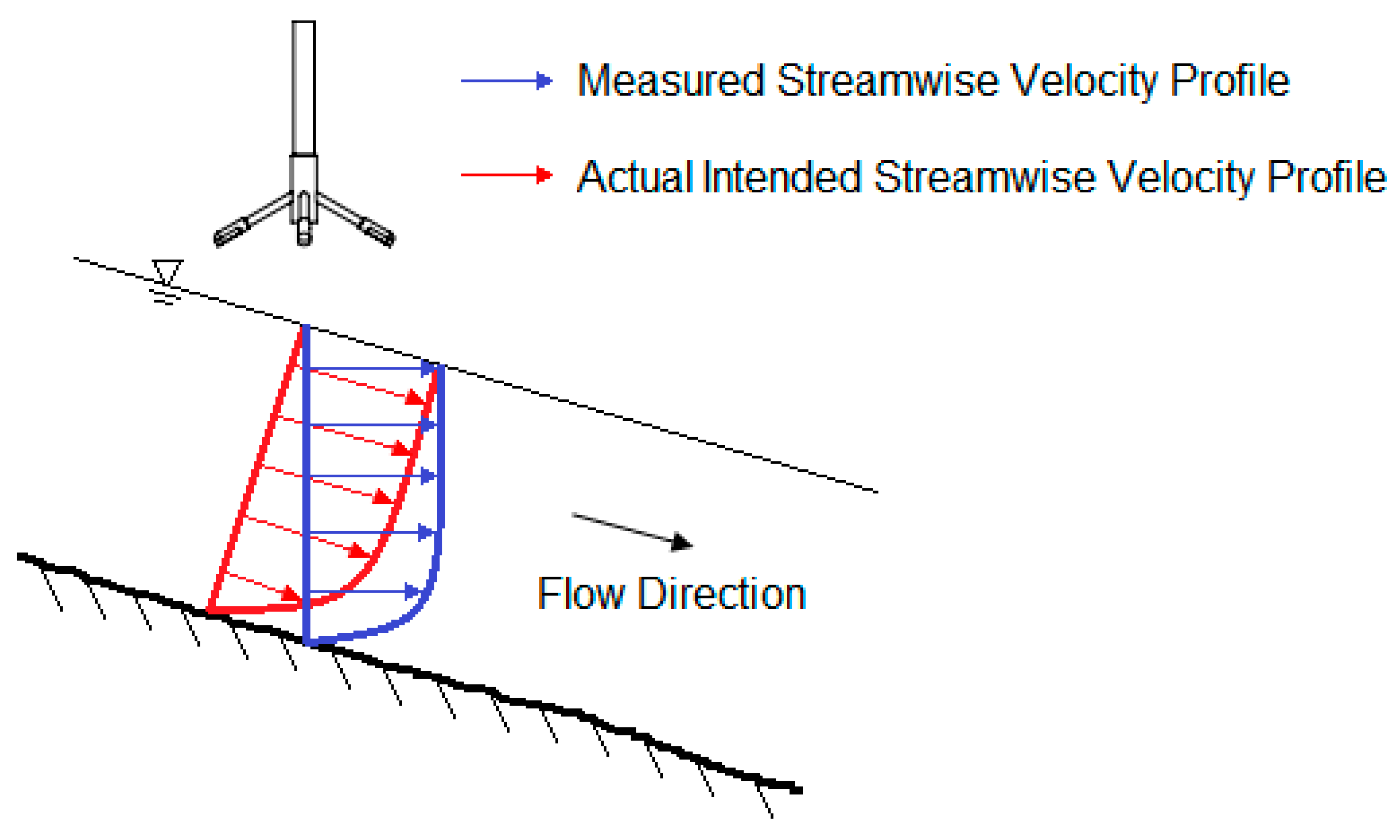
The above-mentioned problem can occur due to misaligned measurements as schematically described by Figure 1, especially in natural channel flows which subject to changing channel characteristics, including irregular side-wall and width conditions [5,6]. In Figure 1, the discrepancy of the measured and intended streamwise flow profiles can result from the bed orientation that displaces the actual measured line from the expected measured line. This is typically difficult to monitor in the natural flow streams where the local bed profile orientation cannot be clearly observed. Due to this reason, there is a crucial need to correct the expected profile to achieve the actual measured profile.
In this paper, we suggest a bed realignment method to correct the measured data with the bed orientation, in order to improve the representativeness of the interpreted profile of an actual measurement. This approach implements a correction factor into the data to recompute the measured profile, and it is applicable to both real-world and experimental flows. The correction factor depends on the bed orientation, and it will affect all the streamwise velocity, turbulence intensity and Reynolds stress profile data. The method realigns the expected profile to the actual location and data and hence minimise their profiles’ in-coherency and discrepancies. Conclusively, the purpose of this study is to investigate and use the proposed correction method to improve the measured data accuracy, which is a crucial step in any field or laboratory hydraulic study.
In order to represent a flow velocity profile, the law of wake proposed by Coles [7] is usually utilised, since it has been proven to reasonably represent the inner and outer flow regions (z/h ratio of <0.2 and z/h ratio of >0.2, respectively) as compared to the law of wall. The turbulence intensity and Reynolds stress, on the other hand, are calculated from the time-averaged Reynolds decomposition of flow velocity. The shear velocity is used to normalise both the velocity and turbulence structure profiles, and by doing this, all different sets of data can be presented together in common scale. To determine the shear velocity, there are two typical approaches, namely using: (1) the Reynolds stress profile extrapolation method and (2) the energy gradient method [8,9]. The extrapolation method can heavily depend on a near-bed Reynolds stress measurement and hence the quality of a near-bed signal-to-noise ratio (SNR) [10]. In comparison, the energy gradient method uses the basic flow parameters such as the hydraulic radius and bed slope, and hence, it should be more error-resistant for ADV measurements as shown by Pu [11], Pu and Shao [12] and Pu et al. [13].
In terms of tested flow conditions, both rough and water-worked bed flows are investigated in this paper. The water-worked rough bed is achieved by long sediment transport and settling processes, where it was introduced by Cooper and Tait [14]. With these tests, this study can fully validate and identify the performance of the proposed bed realignment approach in correcting streamwise velocity and turbulence structure profiles. In addition, the investigation of this study will be concentrated at the near-bed flow region (z/h ratio of <0.2 or <0.4), where the proposed bed alignment method has been found to be most effective.
2. Experimental Descriptions
2.1. Experimental Instrumentations
The utilised flow flume had dimensions of 12 m in length, 0.45 m in width and 0.50 m in height, and it was located at the Hydraulic Laboratory, the University of Bradford, UK [11,13]. In principle, the flume operates in a circulating manner, where an inlet flow is supplied by a storage tank that connects to the outflow of the flume. The water from the storage tank is recirculated into the flume throughout the whole experiment to ensure a sufficient level of seeding within the flow while using an ADV for measurements. The flume has glass walls and a stainless-steel base to provide an initial smooth surface, before the sediment bed is applied to the flume. It is also fitted with a sluice gate at the channel end for controlling the flow depth.
The ADV with down-looking probes was used, which is a product by Nortek Ltd. (Vectrino ADV). It was equipped with a four-probe receiver that can significantly reduce the noise signal of the measurements as compared with a three-probe receiver-equipped ADV [4]. According to the ADV’s manufacturing design, it had a measurement constraint that restricted a 5 cm distance of measurement downward from its probe, which limited the data collection at a 5 cm vertical distance near the water flow surface. However, our key focus is on data collection in the near-bed flow region with ratios of z/h less than 0.4; hence the discussed ADV restriction had no impact on the present study.
2.2. ADV Device
The ADV uses the concept of an acoustic signal emitter–receiver pair to transmit and receive acoustic signals, in order to determine the flow velocity. Since the basic working concept of the ADV involves the frequency pulses transmission, it is sensitive to noise induced by the equipment or the surrounding environment. Parasitical noise, which is induced in the process of ADV measurement, can reduce SNR ratios and cause measurement oscillation [4]. This oscillation is hard to be identified, as it may present a similar form of signal to the velocity turbulence measurement [15].
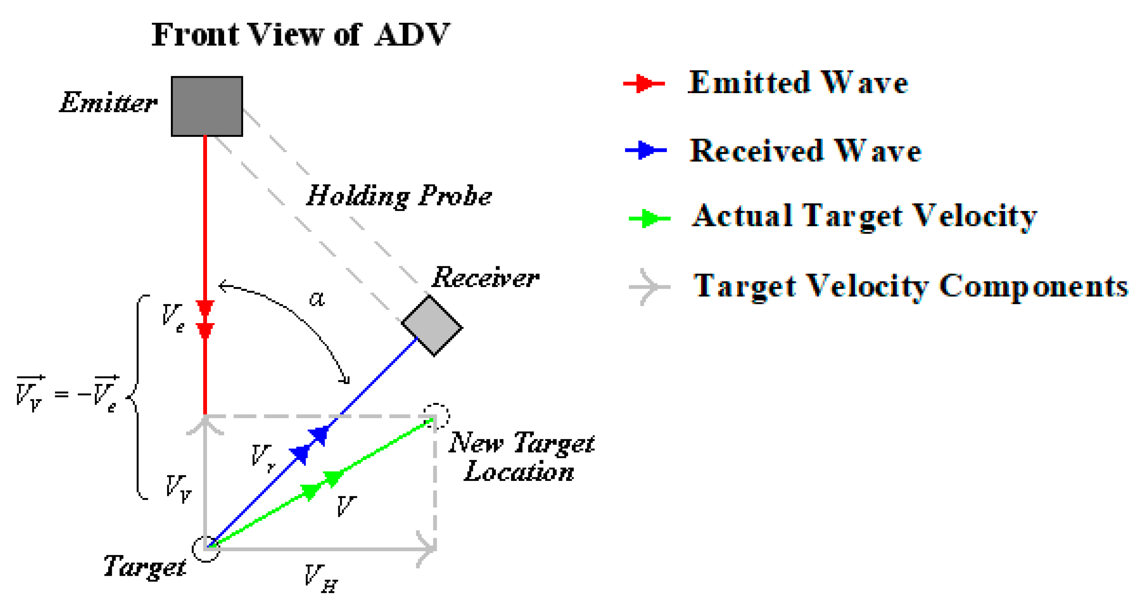
The utilised ADV operates in bistatic mode configuration as presented in Figure 2. In this configuration, the Doppler frequency shift, , can be represented by Equation (1) using the emitted and received frequencies ( and respectively), sound celerity, , and emitter as well as receiver target velocity ( and respectively) (for full derivation, refer to Franca [16]):
where can be determined using the horizontal velocity of the moving target, , and their relationship are presented in Equations (2) (refer to Figure 2 for the illustration of each parameter):
where U, V and W are the velocities of the flow in three dimensions of x, y and z (streamwise, lateral and vertical, respectively), α is the angular difference between the receiver point and the moving target’s point by using the emitter as reference, and β is the angular difference between the probe emitter and the receiver point.
Substituting Equations (1)–(3), the Doppler frequency can be represented in the expression of U, V and W as equation below:
From Equation (4), a velocity matrix solution for a four-receiver ADV configuration can be found as follows:
For a four-receiver ADV, W2 in Equation (5) is introduced as an additional vertical velocity component with the three main velocities. Averaging W1 and W2 can reduce noise signal for the vertical velocity. As proven, the four-receiver ADV had presented velocity measurement with a higher SNR ratio than the three-receiver ADV due to the use of an extra receiver [17].
2.3. Experimental Conditions
A summary has been presented in Table 1 to outline the utilised water-worked and rough bed experimental setups. In order to ensure the self-similarity flow characteristic of a fully developed uniform flow, separate velocity distribution profiles at 3 m, 5 m, 6 m, 7 m and 10 m were measured in the conducted experiments to confirm this uniform flow behaviour. The measured data at the mid-stream profile at 6 m are presented in this paper to represent all uniform flow profiles at different locations within a test.
The point measurements were conducted at multiple vertical positions within a measured location to establish a full flow profile within the near-bed flow region (up to flow with z/h ratios of <0.4). A minimum sampling volume of 1 mm3 was feasible at each sampling point for the utilised ADV; however, this volume would be increased, if the measured point showed a low SNR ratio. All point measurements were recorded at a frequency of 100 Hz for a sampling duration of 5 min.
2.4. Bed Settings
In this paper, the bedform created by the water-worked concept was gradually generated from long sediment transport and settling processes [18]. It was established by several static sediment amour layers. The employed sediment materials were natural river gravels with grain sizes of d16 = 3.81 mm, d50 = 6.62 mm and d84 = 7.94 mm and a density of 2823.8 kg m–3. The natural river gravels were chosen, as it can achieve the water-worked bed condition more rapidly (as compared to sand or silt), where the stationary sediment bed was aimed to be created after long erosion and deposition. d50 was used to estimate the representative Nikuradse’s equivalent roughness ks as suggested by Dey and Raikar [8].
At the start of the water-worked process, the sediment was uniformly fed into the upstream of the flume at a constant rate of 280 g s–1 using a conveyor system. During the whole sedimentation process of amour layers settling, the flow in the water flume was retained at a uniform depth of 100 mm with 40.5 l s–1 of discharge. It took nearly 5 full days of a continuous flash stream for the fully static water-worked rough bed to form, and the nonmovable bed condition was recorded if the average bed level changed throughout the whole channel was less than 0.2d50. After the settling phase was completed, the water depth was increased to 130 mm by the end gate, while the discharge was retained.
This experiment was designed to allow the sediment bed to achieve a nonmoving condition through the flashing of flow, where the sediment critical shear stress was utilised as the benchmark value for its threshold motion. The release rate of sediment in the experiment was estimated by the Meyer-Peter Muller formula as follows [14,18]:
where q* is the dimensionless bedload transport, qb is the bedload transport, s is the relative density between solid and water, g is the gravitational acceleration, d is the sediment size, is the dimensionless critical shear stress, is dimensionless shear stress (), is the bed shear stress, is the water density.
3. Bed Realignment Technique
A three-dimensional (3D) transpose method was used here to consider any small misalignment of the ADV probe. This method proposes a pair matrix of direction–velocity to correct the existed measurement misalignment angle for the time-averaged velocities. The pair matrix is presented as below:
where
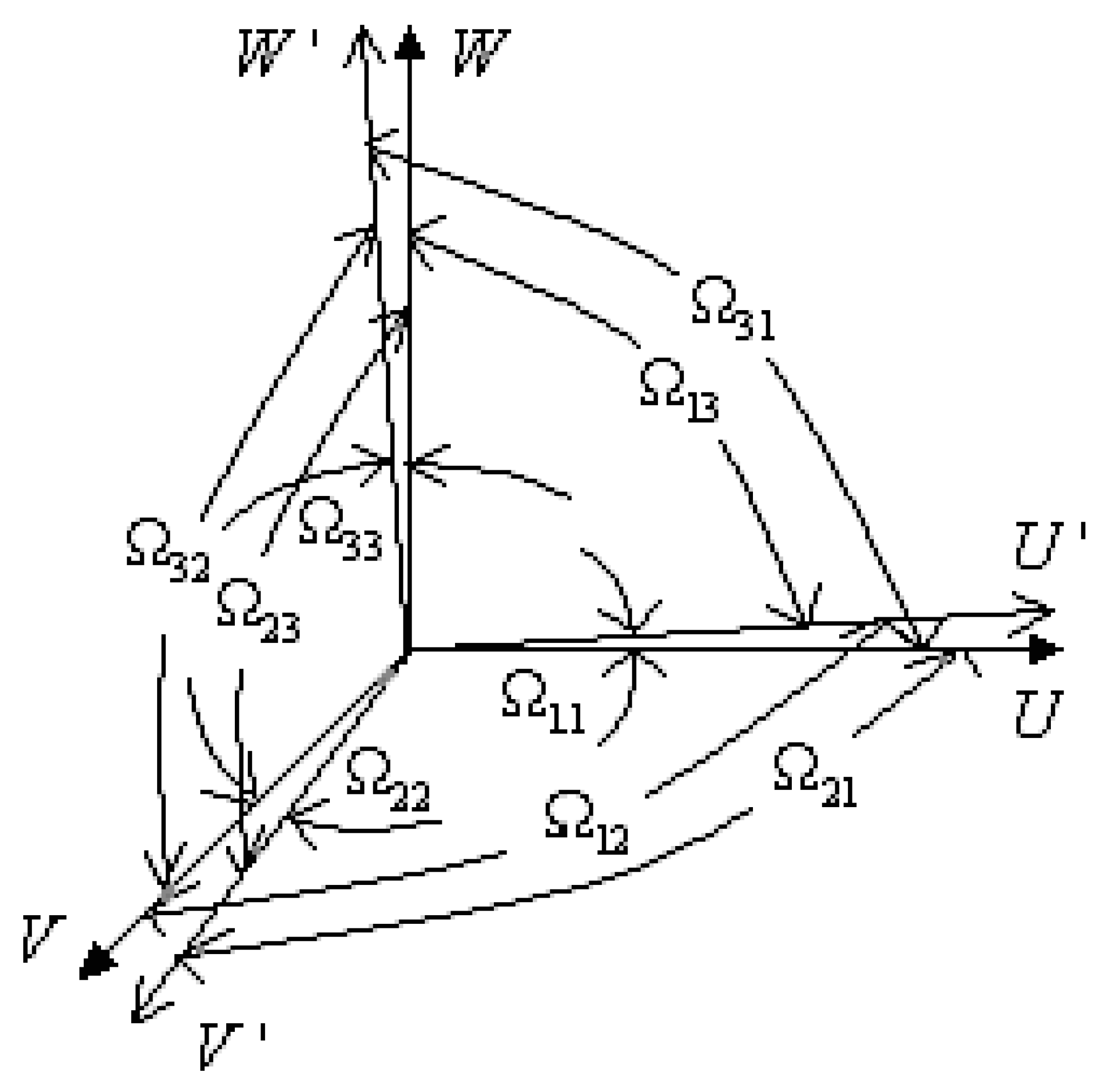
represents the transformed elements of the 3D directions and time-averaged velocities, is the rotational angle between the transformed x-axis and the original x-axis, is the rotational angle between the transformed x-axis and the original y-axis, and so on for the rest of transformation angles (refer to Figure 3 for a definition sketch of the angles in 3D transformation). In Figure 3, is the original axis and is the corrected axis, and the same applied to , , and .
4. Results and Discussion
4.1. Velocity Distribution
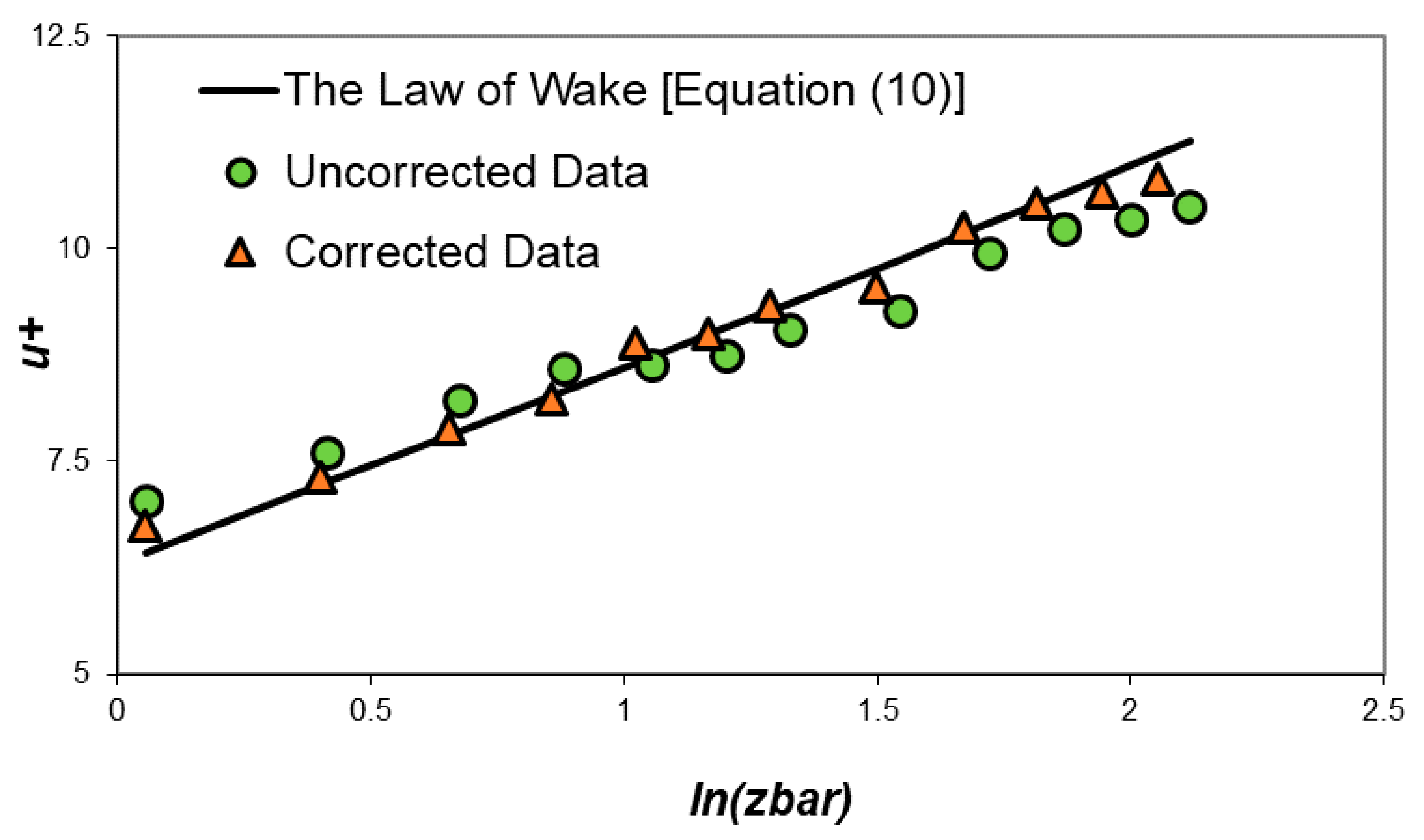
The flow velocity distributions within different well-packed rough bed and sediment transport-induced water-worked bed experiments were analysed, where the studied flow region was focused on z/h ratios of <0.4 to identify different bedform impacts towards the flow. In our comparison, the normalised uniform velocity distribution governed by the law of wake was also utilised as shown below:
where , , is the shear velocity, and zo is the flow reference vertical location from the rough bed crest where zo = 0.25 ks was found to estimate the reference level well. For the rough bed flow, κ = 0.44, Br = 7.4 and П = 0.0792 were used, while κ = 0.44, Br = 6.3 and П = 0.0767 were set for the water-worked bed flow [18]. The shear velocity was estimated as , where g is the gravitational acceleration, R is the hydraulic radius, and So is the bed slope.
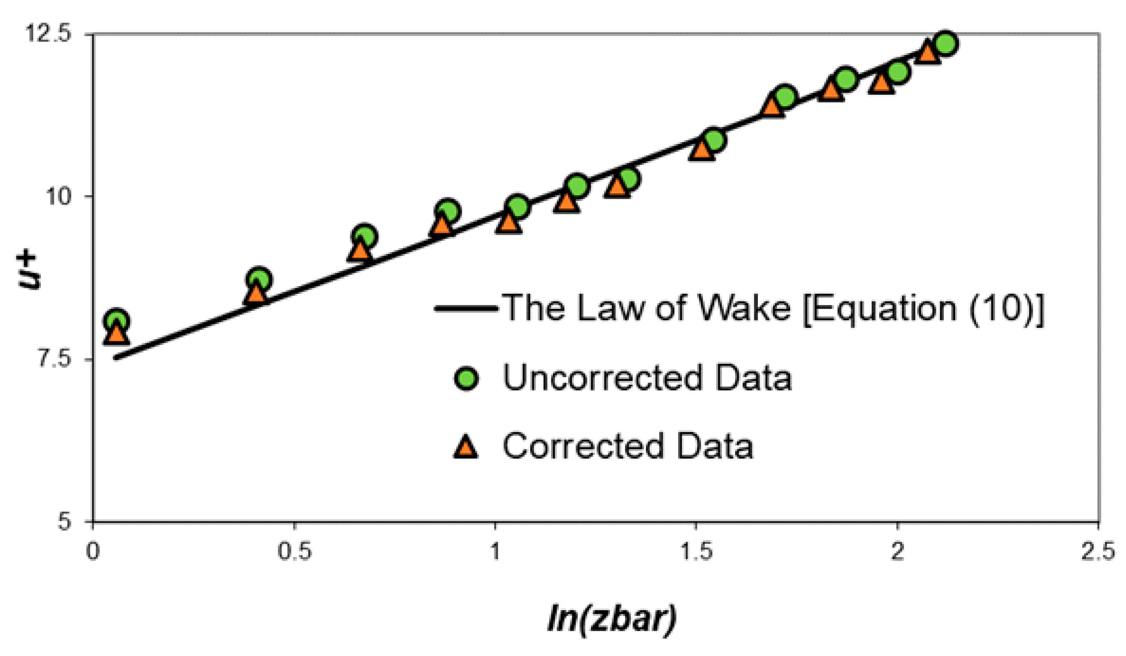
In Figure 4 and Figure 5, the velocity profiles for the rough bed and water-worked bed flows are presented. Comparing the uncorrected and corrected data for the rough bed flow in Figure 4, the latter show a better agreement with the law of wake. The uncorrected data present a regression coefficient of r2 = 0.88, whereas the corrected data show a regression coefficient of r2 = 0.93 when benchmarked by the law of wake. This comparison evidenced that the suggested realignment technique improves the averaged velocity from the measurements; however, the improvement has been proven to be not too significant. In Figure 5, the same comparison has been performed for the corrected and uncorrected data for the water-worked bed after long sediment flushing and settling. The uncorrected data give a regression coefficient of r2 = 0.71 compared to the law of wake; but this regression has been enhanced to r2 = 0.94 for the corrected data. With this finding, we can conclude that the proposed realignment method works reasonably well on the rough bed flow, but it improves the velocity point-measurement data of the water-worked bed more clearly.
The bedform created by the water-worked bed had a higher ks value and more unpredictable law of wake’s constants and therefore present a more difficulty scenario for accurate near-bed velocity profile measurements especially at z/h ≤ 0.2 (as suggested by Cooper and Tait [14]; Pu et al. [18]). Referred to Figure 5, the near-bed velocity correction has been well performed to achieve high agreement with the calculated law of wake, and this demonstrates that the proposed method works for the flow within the sediment transport-induced water-worked bed. Practically, the presented method can also be used in field measurements to improve the real-world flow data.
4.2. Turbulent Intensity Comparison
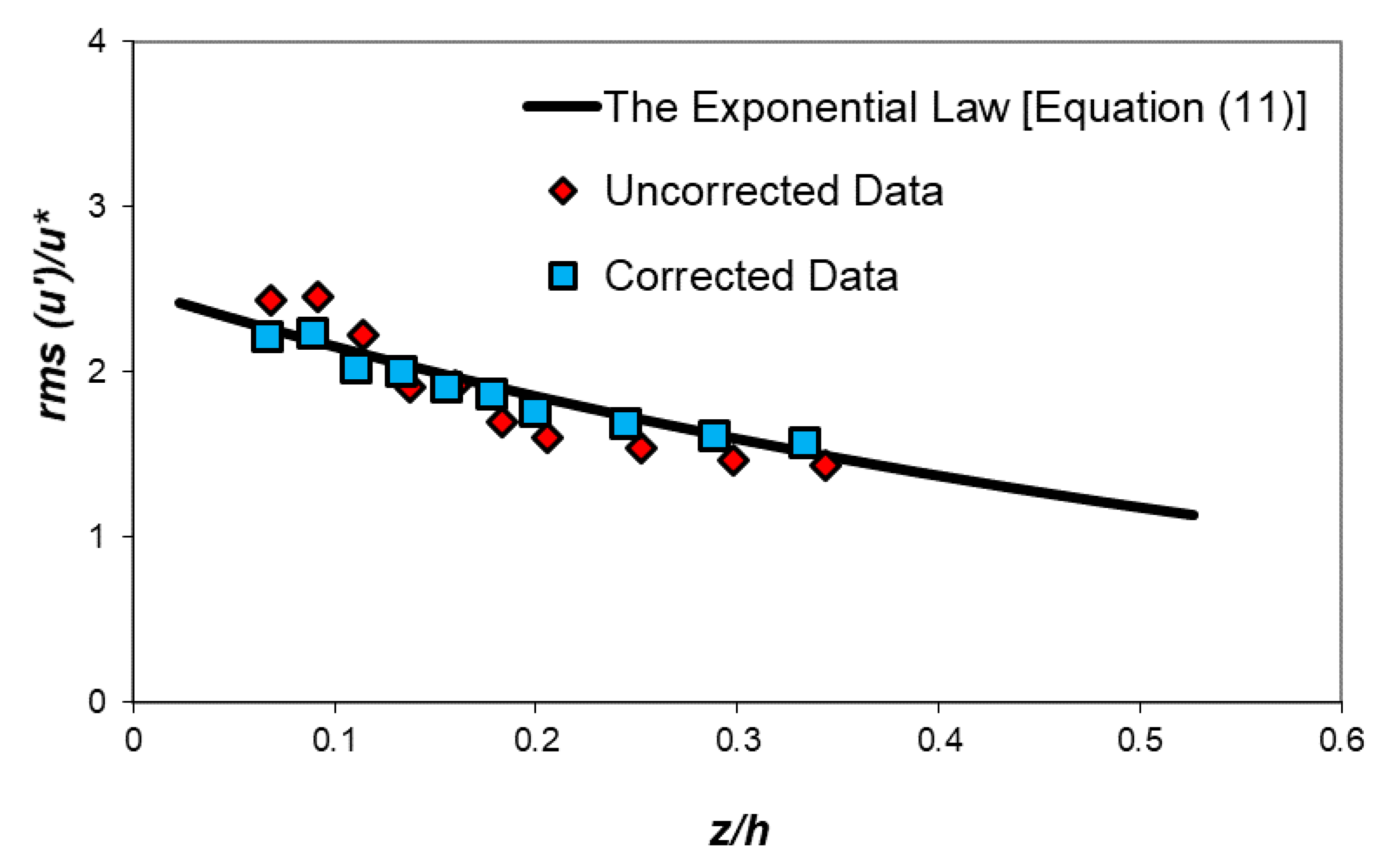
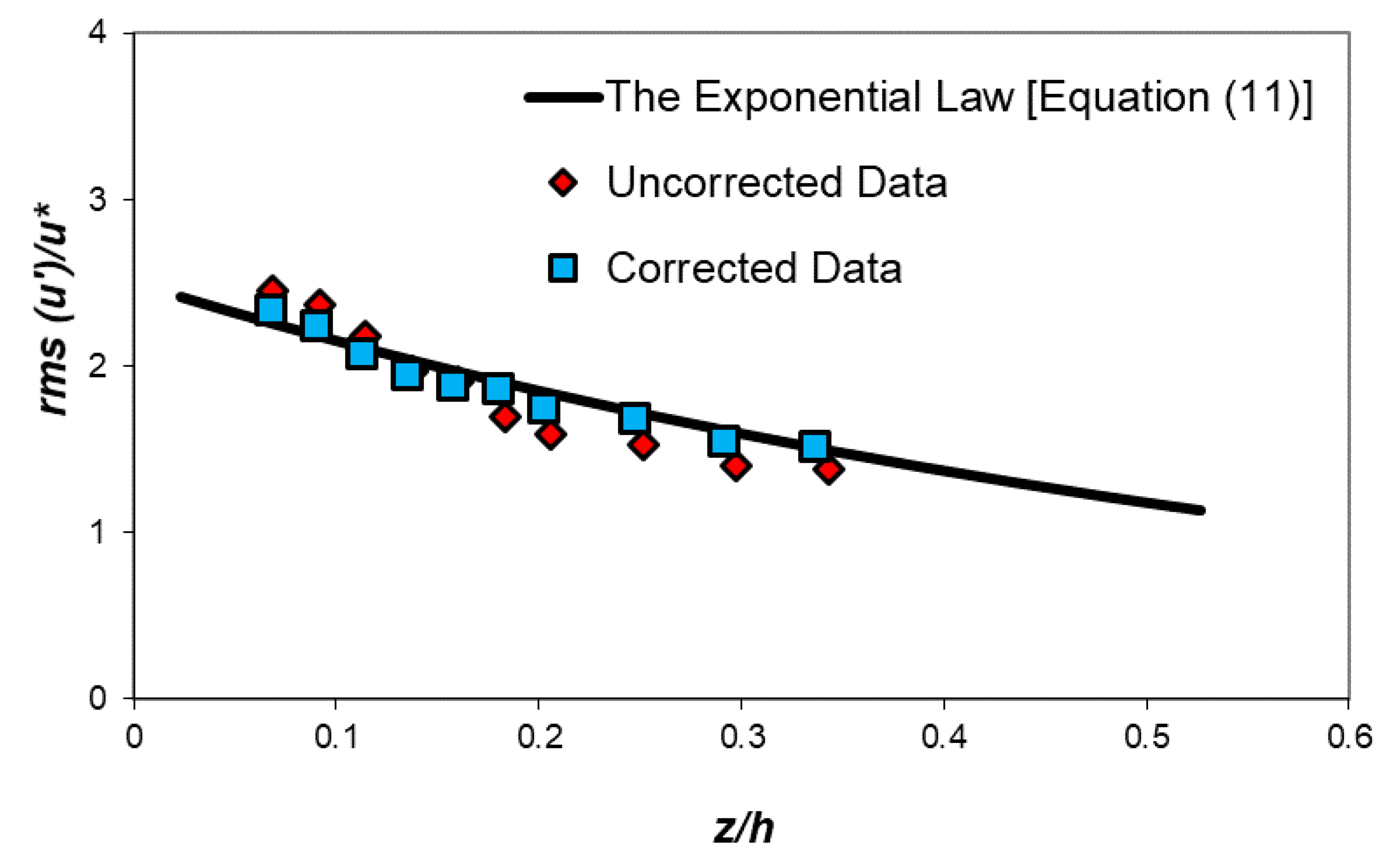
Theoretically, the streamwise turbulent intensity represents a more dominant element compared to the transverse and vertical turbulent intensities in a flow. However, it is also more sensitive towards point measurement anomalies or misalignment [11,19]. We carried out the comparison of the measured turbulent intensity data to the reported exponential law to investigate their discrepancy. The utilised turbulence intensity’s exponential law has been proposed by Nezu and Nakagawa [20] as below:
where u′ is the velocity fluctuations in streamwise direction, and A and λ are empirical constants for turbulence intensities. One can observe from Figure 6 and Figure 7 that the exponential law represents the measured rough and water-worked bed flows’ turbulence intensity profiles well. In Figure 6 for the rough bed, the uncorrected data have a regression coefficient of r2 = 0.79 while the corrected data give r2 = 0.91 based on the comparison with the exponential law. On the other hand, Figure 7 shows the uncorrected and corrected data’s regression coefficients to be r2 = 0.82 and r2 = 0.90, respectively. From Figure 6 and Figure 7, the well-packed rough and water-worked bed flows showed a similar magnitude of improvement in regression coefficient when the proposed realignment method was applied. This proved that the turbulent intensity dictated by the unidirectional velocity fluctuation can be improved by the proposed method; but the improvement on sediment transport-induced bedform (i.e., water-worked bed) is similar to the experimentally prepared bed. Due to this, it will be also crucial to investigate the effectiveness of the proposed approach to correct the multidirectional velocity fluctuations. In the view of this reason, we will be further investigating the Reynolds stress comparison in the coming section.
4.3. Reynolds Stress Comparison
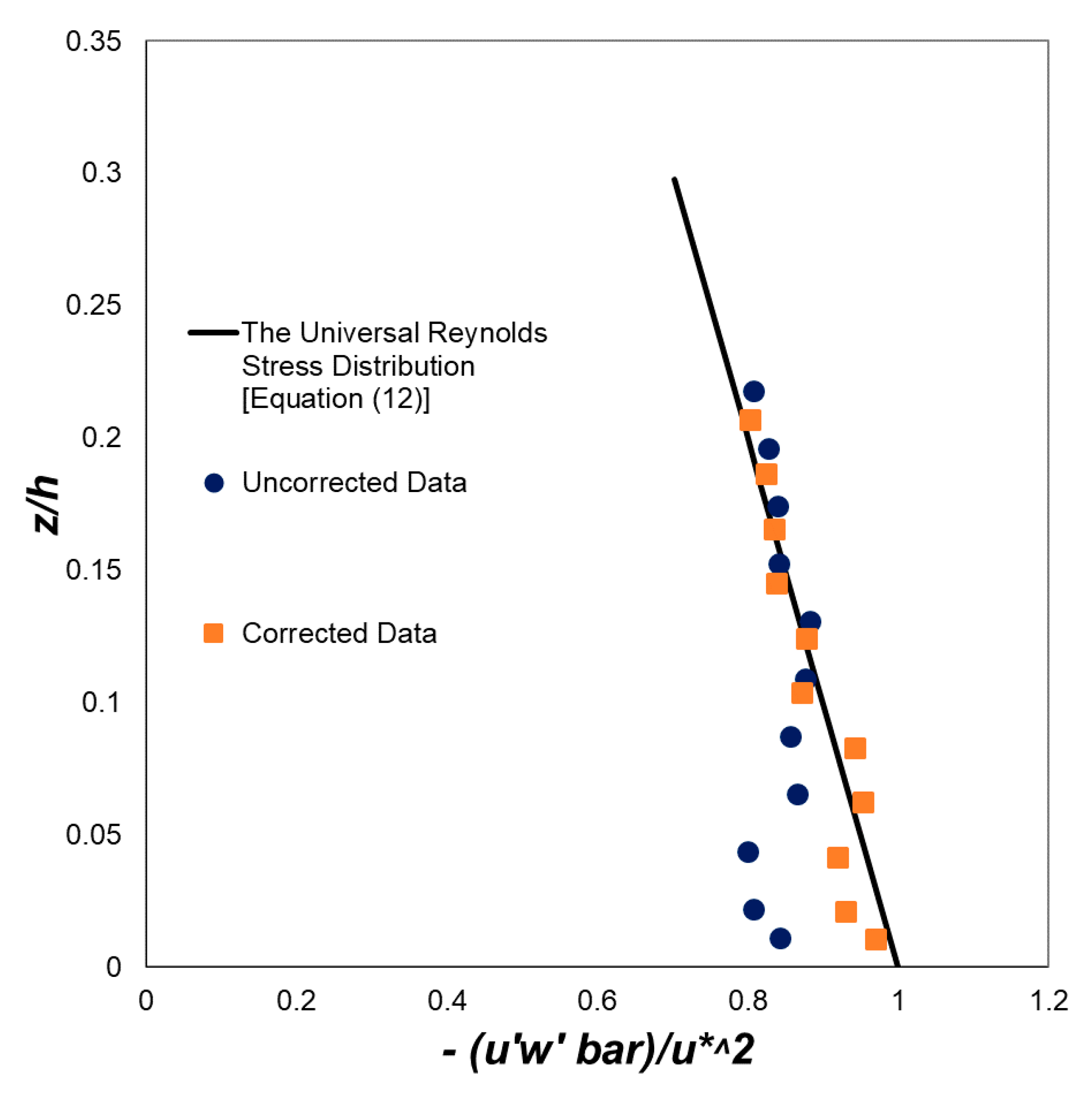
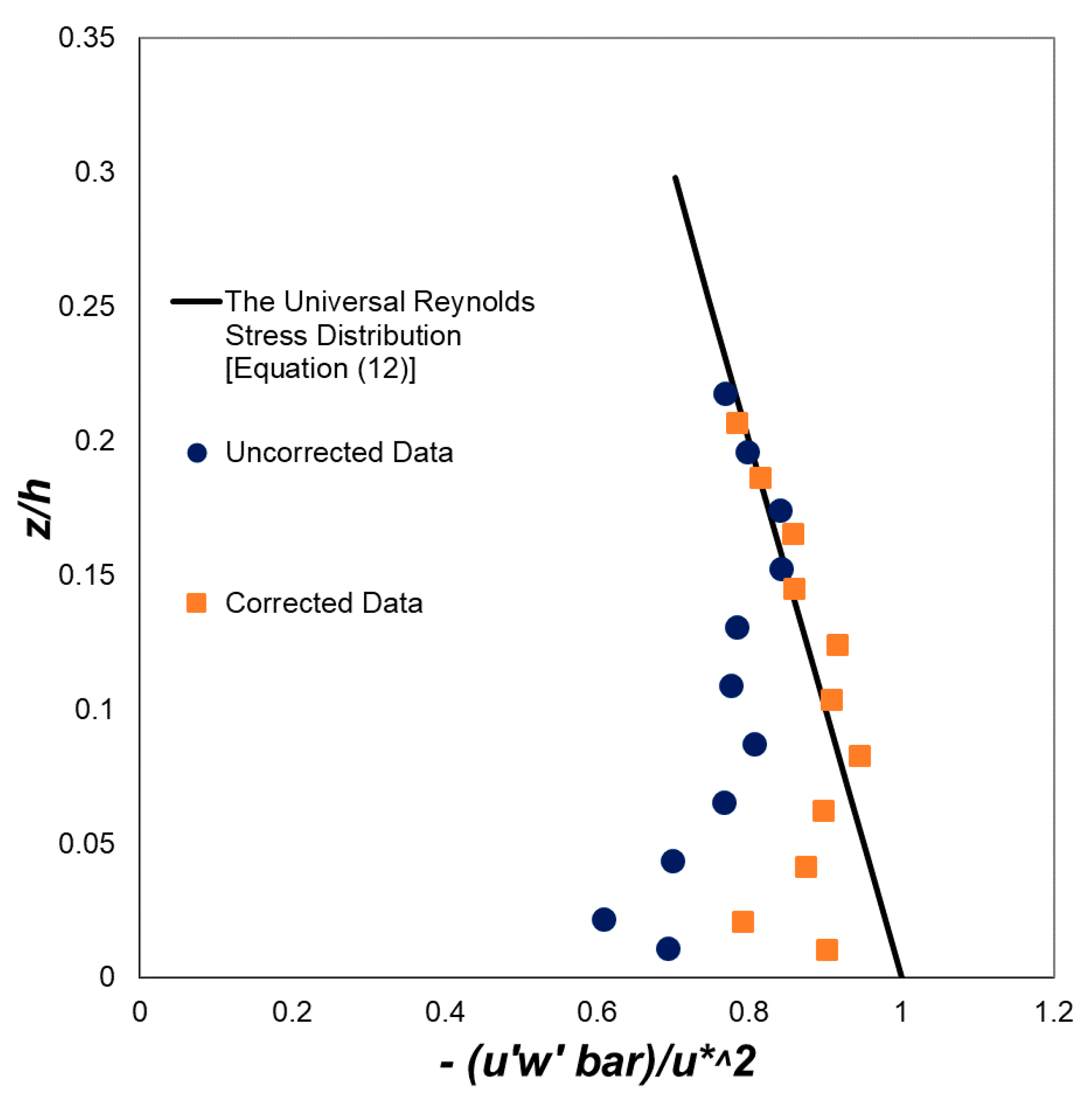
The universal distribution calculation has usually been suggested to represent the normalised Reynolds stress in different bedforms [8,20], which is shown as below:
Figure 8 and Figure 9 were produced to inspect the performance of the proposed realignment method in rectifying the measured velocity fluctuations in U and W components (i.e., in the form of Reynolds stress). The results in Figure 8 and Figure 9 illustrated that the proposed technique improved the measured data (as showing by the comparison between the corrected and uncorrected data). The observation has been focused on z/h ratios of ≤0.2 only, as it was found that the profiles above this limit converged well into the universal distribution.
More specifically, at z/h ratios of ≥0.1 for the rough bed and z/h ratios of ≥0.15 for the water-worked bed, the difference between the universal distribution and the uncorrected measurements was clear. The convergence of the measured data into the universal distribution was improved in the lower location (i.e., by z/h ratio ≈ 0.05 for the rough bed, and z/h ratio ≈ 0.75 for the water-worked bed) for the corrected data, which demonstrated the capability of the proposed realignment method. In addition, the sediment transport-formed water-worked bed created a thicker bed shear layer compared to the well-packed rough bed produced experimentally due to the rougher surface presented by the former. As a result, the Reynolds stress unconverged region in the near-bed region was larger for the water-worked bed flow. As agreed by the recent studies [21,22], both the bedload transport and water-worked bed at experimental and field studies can significantly alter the turbulence structure profile, particularly in the near-bed region. Thus, the enhanced accuracy of near-bed turbulence structure measurements by the proposed approach will aid the researches in achieving trustable data of flow–bed interactions.
5. Conclusions
This paper proposed a bed realignment method to improve the measured velocity-related data of the sediment transport-induced water-worked and experimentally prepared well-packed bed flows. The comparisons by velocity profile, streamwise turbulent intensity and Reynolds stress were investigated to identify the capability of the proposed method at those flows. Through this study’s findings, significant measured data improvement has been achieved in the Reynolds stress data which involve multidirectional velocity fluctuation analysis. For time-averaged velocity and turbulent intensity that involve velocity in a unidimension (i.e., streamwise), the improvement was not as drastic as for the Reynolds stress. Overall, the results validated the functioning of the proposed bed realignment method to correct the measured data by ADV point measurements, in terms of giving a closer correspondence to the theoretical laws.
Funding
This research received no external funding.
Institutional Review Board Statement
Not applicable.
Informed Consent Statement
Not applicable.
Data Availability Statement
The data presented in this study are available on reasonable request from the author.
Conflicts of Interest
The author declares no conflict of interest.
References
- Cea, L.; Puertas, J.; Pena, L. Velocity measurement on highly turbulent free surface flow using ADV. Exp. Fluids 2007, 42, 333–348. [Google Scholar] [CrossRef]
- Goring, D.G.; Nikora, V.I. Despiking acoustic doppler velocimeter data. J. Hydraul. Eng. 2002, 128, 117–126. [Google Scholar] [CrossRef] [Green Version]
- Kraus, N.C.; Lohrmann, A.; Cabrera, R. New acoustic meter for measuring 3D laboratory flows. J. Hydraul. Eng. 1994, 120, 407–412. [Google Scholar] [CrossRef]
- Blanckaert, K.; Lemmin, U. Means of noise reduction in acoustic turbulence measurements. J. Hydraul. Res. 2006, 44, 1–15. [Google Scholar] [CrossRef]
- Pu, J.H.; Pandey, M.; Hanmaiahgari, P.R. Analytical modelling of sidewall turbulence effect on streamwise velocity profile using 2D approach: A comparison of rectangular and trapezoidal open channel flows. J. Hydro Environ. Res. 2020, 32, 17–25. [Google Scholar] [CrossRef]
- Pu, J.H. Turbulent rectangular compound open channel flow study using multi-zonal approach. Environ. Fluid Mech. 2018, 19, 785–800. [Google Scholar] [CrossRef] [Green Version]
- Coles, D. The law of the wake in the turbulent boundary layer. J. Fluid Mech. 1956, 1, 191–226. [Google Scholar] [CrossRef] [Green Version]
- Dey, S.; Raikar, R.V. Characteristics of loose rough boundary streams at near-threshold. J. Hydraul. Eng. 2007, 133, 288–304. [Google Scholar] [CrossRef]
- Song, T.; Chiew, Y.M. Turbulence measurement in nonuniform open-channel flow using acoustics Doppler velocimeter (ADV). J. Eng. Mech. 2001, 127, 219–232. [Google Scholar] [CrossRef]
- Yu, G.; Tan, S.K. Errors in bed shear stress as estimated from vertical velocity profile. J. Irrig. Drain. Eng. 2006, 132, 490–497. [Google Scholar] [CrossRef]
- Pu, J.H. Efficient Finite Volume Numerical Modelling and Experimental Study of 2D Shallow Water Free Surface Turbulent Flows. Ph.D. Dissertation, University of Bradford, Bradford, UK, 2008. [Google Scholar]
- Pu, J.H.; Shao, S. Non-uniform open channel flows study using three-dimensional turbulence measurements. In Proceedings of the 35th International IAHR World Congress, Chengdu, China, 8–13 September 2013; Article A10326. pp. 1–10. [Google Scholar]
- Pu, J.H.; Shao, S.; Huang, Y. Numerical and experimental turbulence studies on shallow open channel flows. J. Hydro Environ. Res. 2014, 8, 9–19. [Google Scholar] [CrossRef] [Green Version]
- Cooper, J.R.; Tait, S.J. The spatial organisation of time-averaged streamwise velocity and its correlation with the surface topography of water-worked gravel beds. Acta Geophys. 2008, 56, 614–642. [Google Scholar] [CrossRef]
- Mori, N.; Suzuki, T.; Kakuno, S. Noise of Acoustic Doppler Velocimeter Data in Bubbly Flows. J. Eng. Mech. 2007, 133, 122–125. [Google Scholar] [CrossRef]
- Franca, M. A Field Study of Turbulent Flows in Shallow Gravel-Bed Rivers. Ph.D. Thesis, École Polytechnique Fédérale De Lausanne, Lausanne, Switzerland, 2005. [Google Scholar]
- Rusello, P.J.; Lohrmann, A.; Siegel, E.; Maddux, T. Improvements in Acoustic Doppler Velocimetery. In Proceedings of the 7th International Conference on Hydroscience and Engineering (ICHE-2006), Philadelphia, PA, USA, 7 July 2006; pp. 1–16. [Google Scholar]
- Pu, J.H.; Wei, J.; Huang, Y. Velocity Distribution and 3D Turbulence Characteristic Analysis for Flow over Water-Worked Rough Bed. Water 2017, 9, 668. [Google Scholar] [CrossRef] [Green Version]
- Pu, J.H.; Tait, S.; Guo, Y.; Huang, Y.; Hanmaiahgari, P.R. Dominant Features in Three-Dimensional Turbulence Structure: Comparison of Non-Uniform Accelerating and Decelerating Flows. Environ. Fluid Mech. 2018, 18, 395–416. [Google Scholar] [CrossRef] [Green Version]
- Nezu, I.; Nakagawa, H. Turbulent Open-Channel Flows; IAHR Monograph, A. A. Balkema: Rotterdam, The Netherlands, 1993. [Google Scholar]
- Cooper, J.R.; Ockleford, A.; Rice, S.P.; Powell, D.M. Does the Permeability of Gravel River Beds Affect Near-bed Hydrodynamics? Earth Surf. Process. Landf. 2018, 43, 943–955. [Google Scholar] [CrossRef] [Green Version]
- Khosravi, K.; Chegini, A.H.N.; Cooper, J.R.; Daggupati, P.; Binns, A.; Mao, L. Uniform and graded bed-load sediment transport in a degrading channel with non-equilibrium conditions. Int. J. Sediment Res. 2020, 35, 115–124. [Google Scholar] [CrossRef]
Figure 1.
Discrepancy between the measured and actual intended flow velocity profiles.

Figure 2.
Working principle of a bistatic acoustic Doppler velocimeter (ADV) configuration.

Figure 3.
Three-dimensional (3D) rotational axes of the bed realignment method.

Figure 4.
Normalised velocity profile over the laboratory-prepared well-packed rough bed.

Figure 5.
Normalised velocity profile over the sediment transport-induced water-worked bed.

Figure 6.
Normalised turbulent intensity over the laboratory-prepared well-packed rough bed.

Figure 7.
Normalised turbulent intensity over the sediment transport-induced water-worked bed.

Figure 8.
Normalised Reynolds stress over the well-packed laboratory-prepared rough bed.

Figure 9.
Normalised Reynolds stress over the sediment transport-induced water-worked bed.


Table 1.
Basic experimental conditions for flow tests.
| Bed Condition | Q (l s−1) | U (m s−1) | h (m) | Fr (-) | u (m s−1) |
|---|---|---|---|---|---|
| Well-packed rough | 40.5 | 0.69 | 0.13 | 0.61 | 0.054 |
| Water-worked | 40.5 | 0.69 | 0.13 | 0.61 | 0.060 |
Publisher’s Note: MDPI stays neutral with regard to jurisdictional claims in published maps and institutional affiliations. |
© 2021 by the author. Licensee MDPI, Basel, Switzerland. This article is an open access article distributed under the terms and conditions of the Creative Commons Attribution (CC BY) license (http://creativecommons.org/licenses/by/4.0/).
Share and Cite
MDPI and ACS Style
Pu, J.H. Velocity Profile and Turbulence Structure Measurement Corrections for Sediment Transport-Induced Water-Worked Bed. Fluids 2021, 6, 86. https://0-doi-org.brum.beds.ac.uk/10.3390/fluids6020086
AMA Style
Pu JH. Velocity Profile and Turbulence Structure Measurement Corrections for Sediment Transport-Induced Water-Worked Bed. Fluids. 2021; 6(2):86. https://0-doi-org.brum.beds.ac.uk/10.3390/fluids6020086
Chicago/Turabian StylePu, Jaan H. 2021. "Velocity Profile and Turbulence Structure Measurement Corrections for Sediment Transport-Induced Water-Worked Bed" Fluids 6, no. 2: 86. https://0-doi-org.brum.beds.ac.uk/10.3390/fluids6020086