
Modeling Immiscible Fluid Displacement in a Porous Medium Using Lattice Boltzmann Method
by
 ,
,
Magzhan Atykhan
1 ,
,
Bagdagul Kabdenova (Dauyeshova)
1,
Ernesto Monaco
2 and
Luis R. Rojas-Solórzano
1,*
1
Department of Mechanical and Aerospace Engineering, School of Engineering and Digital Sciences, Nazarbayev University, Nur-Sultan 010000, Kazakhstan
2
Engineering Software Steyr (ESS), Berggasse 35, 4400 Steyr, Austria
*
Author to whom correspondence should be addressed.
Fluids 2021, 6(2), 89; https://0-doi-org.brum.beds.ac.uk/10.3390/fluids6020089
Submission received: 20 September 2020
/
Revised: 12 January 2021
/
Accepted: 20 January 2021
/
Published: 22 February 2021
(This article belongs to the Special Issue Convective Instability in Porous Media, Volume II)
Abstract
:The numerical investigation of the interpenetrating flow dynamics of a gas injected into a homogeneous porous media saturated with liquid is presented. The analysis is undertaken as a function of the inlet velocity, liquid–gas viscosity ratio (D) and physical properties of the porous medium, such as porous geometry and surface wettability. The study aims to improve understanding of the interaction between the physical parameters involved in complex multiphase flow in porous media (e.g., CO2 sequestration in aquifers). The numerical simulation of a gaseous phase being introduced through a 2D porous medium constructed using seven staggered columns of either circular- or square-shaped micro-obstacles mimicking the solid walls of the pores is performed using the multiphase Lattice Boltzmann Method (LBM). The gas–liquid fingering phenomenon is triggered by a small geometrical asymmetry deliberately introduced in the first column of obstacles. Our study shows that the amount of gas penetration into the porous medium depends on surface wettability and on a set of parameters such as capillary number (Ca), liquid–gas viscosity ratio (D), pore geometry and surface wettability. The results demonstrate that increasing the capillary number and the surface wettability leads to an increase in the effective gas penetration rate, disregarding porous medium configuration, while increasing the viscosity ratio decreases the penetration rate, again disregarding porous medium configuration.
1. Introduction
The increase in greenhouse gas (GHG) concentration in the atmosphere over the past decades has generated strong interest in developing technologies that help in reducing CO2 emissions, especially those generated by fossil fuel combustion in heat and power generation [1,2,3]. Carbon dioxide sequestration, a fundamental part of a larger Carbon Capture and Storage (CCS) initiative [4], is an emerging field of research that is viewed as one of the potential solutions to decrease CO2 concentration in the atmosphere. CCS is based on two main stages [5,6]. Firstly, it requires the capture of carbon dioxide from industrial and energy sources, and, secondly, it needs to transport and store it for long-term sequestration in underground aquifers, which are essentially porous media saturated with saline water isolated from the atmosphere. The penetration of a displacing fluid into a porous medium depends on the capillary and viscous forces at work, as well as the physical properties of the porous medium itself [7]. The displacement of the non-wetting fluid by the wetting phase is essential and affects CO2 sequestration in terms of storage efficiency, capacity, and security. However, it is a rather complex phenomenon, difficult to study in laboratory or through purely analytical means. Numerical modeling is a complementary and powerful approach that can greatly help in understanding this phenomenon, provided that the discretized model is capable of capturing the rich physics involved in such a process.
Despite the continuous increase in computational power, modelling multiphase flow in a porous medium is challenging for conventional Computational Fluid Dynamics (CFD) tools due to the complex geometries involved, including small length-scale pores, and, hence, the required use of a computationally prohibitive adapted mesh [8]. For such meso-scale phenomena, the multiphase Lattice Boltzmann Method (LBM) has proved to be a promising alternative to standard CFD techniques [8,9]. Among these techniques, the volume-of-fluid (VOF) [10], the level set (LS) [11] and the phase field (PF) [12] methods are most common. However, according to Yang and Boek [7], these techniques have numerical instabilities at small-scale interface regions.
The LBM reproduces the macroscopic continuous dynamics of fluids, starting from the statistical approach embedded in the Kinetic Theory, in which the microscopic, discrete nature of a fluid can be described by particle distribution functions while avoiding the necessity to track individual molecules [9,10,11]. Additionally, in comparison to traditional CFD tools, the LBM algorithm is intrinsically parallel and effective in dealing with complex boundary geometries [13,14]. Since the very early stages of LBM, several multiphase models have been proposed, namely the color-fluid model, the pseudo-potential model, the free energy model and the mean-field theory model [15,16,17]. Despite the many advantages of LBM, all these multicomponent multiphase models are confined to use for small liquid–gas density ratios due to the presence of spurious currents at the interface, which ultimately promote numerical instabilities [18,19,20,21]. According to Fakhari and Rahiman [22], LBM multicomponent multiphase models have a limited range of gas–liquid density ratios (up to 15) due to these numerical instabilities. Generally, if the magnitude of the unphysical currents corresponds to the order of the local flow velocity, the model generates meaningless results [14].
There have been several attempts to improve the performance of multiphase LBM at high density ratios. For example, Inamuro et al. [23] proposed using a lattice kinetic scheme, which applies a single equilibrium distribution function calibrating the speed of sound, while Lee et al. [24] introduced a new method, which is based on a pressure equation and can be applied to a wide range of density ratios. Additionally, in the approach by Lee et al., spurious velocities at the interface are drastically reduced by increasing the surface thickness. Moreover, Yuan and Schaefer [25] studied the stability of LBM at high density ratios under various equation of states (EOS). It was found that Peng–Robinson (P-R) and Carnahan–Starling (C-S) EOS can model high-density ratios while minimizing the effects of spurious velocities because these EOS allow LBM to correctly capture the fluid flow phenomena in terms of temperature, in addition to other relevant thermodynamic parameters. Furthermore, Fakhari et al. [26] have found that the flow through the pore domain is extremely sensitive to the choice and accuracy of the boundary conditions, especially the entrance conditions.
Well-known numerical studies on porous media apply multiphase color-fluid LBM [6,17,27,28] with a density ratio of 1. However, the pseudo-potential model has shown better performance in terms of stability for fluid flows involving higher density contrasts, as, for example, in the case of CO2 flow in porous media [25]. According to Li et al. [29], Kupershtokh et al. [30], Chen et al. [31] and Yuan-Schaefer [25], the performance of the model depends on EOS and the forcing scheme. There are different forcing schemes, such as velocity-shift, exact difference method (EDM) and Guo’s forcing scheme, depending on how interaction force is introduced into LBM. The accuracy and stability of these forcing schemes have been analyzed in several studies [16,29,30,31]. According to Li et al. [29], EDM is more stable when relaxation time is less than 1, i.e., , while a velocity-shift forcing scheme is more stable when . Li et al. [29] also analyzed the effects of different values of on the coexistence curves. However, in a previous study, Kupershtokh et al. [30] showed that at , EDM and velocity-shift forcing schemes are identical. Due to the fact that LBM is still a newly emerging method, there are contradictions between some studies. Therefore, in this study we compare these two popular forcing schemes in terms of numerical stability and accuracy and make recommendations regarding multiphase flows in complex geometries, where a model’s high stability is crucial.
We use P-R EOS in this study, as it is one of the accurate EOS, which helps specify the fluid thermodynamic properties through their acentric factor. We study the displacement process and its efficiency by applying pseudo-potential LBM instead of the widely used color fluid model. Throughout our work, the gas is injected with a uniform inlet profile into a saturated aquifer at different viscosity ratios, capillary numbers and pore geometry. By changing these parameters, their effects on displacement efficiency are investigated. The liquid–gas density ratio is fixed at 5 to ensure negligible spurious velocities at the interface. This apparently low-density ratio is also consistent with carbon dioxide injection condition in deep saline aquifers, which typically occurs at critical or near-critical regimes.
2. Methodology
2.1. Lattice Boltzmann Method
In this study, the standard two-dimensional Lattice Boltzmann Method (LBM) with a Bhatnagar–Gross–Krook (BGK) collision operator is used. The Lattice Boltzmann Equation (LBE), which describes the rate of change of the particle distribution function in a generic point x on a Cartesian grid at a generic time t on a single direction of a predefined lattice, is given by Equation (1):
where is the particle velocity distribution function associated with i-th direction of the lattice, is the time increment and the lattice speed along the i-th direction. is the body force term. τ expresses the dimensionless relaxation time, which is used to describe the kinematic viscosity . M is the number of discrete velocities and cs is the speed of sound. The number and directions of the set of M speeds define the lattice, which is typically referred to as DnQM, n being space dimensionality. Since the goal is to obtain the Navier–Stokes (NS) equations, a given lattice is acceptable if and only if it possesses enough symmetries to recover 4th-order isotropy of stress–strain tensors [8]. is the corresponding equilibrium distribution function described as follows:
where u is the macroscopic velocity and is the weighting factor [25]. The form of Equation (2) is designed to recover the Euler equation. In this two-dimensional study, we adopt the widely used D2Q9 lattice, which is characterized by the following weighting factors (see Table 1):
These weighting factors are necessary to recover isotropy for lattice models with different velocity vector modules. Macroscopic quantities like density and momentum density can be recovered as discrete moments of the distribution functions, which are given by Equations (3) and (4), respectively. Additionally, in LBM, the incompressible NS equations with pressure are recovered via simple EOS rather than by solving a Poisson equation, as in standard CFD [32]. The ideal EOS with standard LBE is described in Equation (5).
The LBE described so far accounts for single-phase problems; to deal with multiphase flows, non-ideal effects must be introduced. In this study, we chose the pseudo-potential, or Shan–Chen [32], model, which consists of introducing a body force depending on the discrete gradient of a function of density, usually referred to as effective mass (Equation (6)).
where is the Green’s function, which describes the interaction strength between neighbour particles. Depending on its magnitude, the interaction force can be described as repulsive or attractive. is the effective mass, which controls the EOS and, thus, the nature of the non-ideal fluid to be modeled. The SC model leads to the general EOS given by:
The adhesion force between two fluids is expressed by Equation (8):
where is the interaction force between the fluid and solid walls. The interaction can be considered as non-wetting or wetting depending on its magnitude. Specifically, it is considered positive for a non-wetting fluid surface and negative for a wetting fluid surface [33]. To calculate the contact angle, the modified Young’s equation is used as proposed by Huang et al. [34]:
where
is cohesion parameter,
is calculated from Equation (8) and
is the density factor.
The Shan–Chen EOS is widely used for multiphase LBM simulations due to its simplicity (Equation (7)). However, in this study, the Peng–Robinson EOS [35] (Equations (10) and (11)) is preferred because it has proven to be capable of dealing with higher density ratios with a reduction in the instabilities associated with spurious currents [25].
where R is the universal gas constant, a () and b () are species-dependent coefficients, denotes a function of the reduced temperature (, is the critical temperature of the fluid in consideration) and is the so-called acentric factor. In the present work, the values of a, b and R are set as 2/49, 2/21 and 1, respectively; thus, the critical properties of the LBM fluid are evaluated correspondingly.
2.2. Forcing Scheme Analysis
According to Kuperstokh et al. [30], the exact difference method (EDM) considers additional body forces to avoid discrepancies of distribution function at the higher-order terms of conservation laws. EDM can be derived from LBM by discretization of LBE in the velocity space. Finally, the body force term of the distribution function can be written as:
where, is change of mass velocity at a node. is equal to the difference in equilibrium distribution functions during time-step at constant density .
The performance of the pseudo-potential model with both a velocity-shift forcing scheme and an EDM scheme was investigated at different relaxation times. Figure 1 shows the lowest achievable reduced temperature (T/Tc) for both schemes at τ < 1. Results from these tests show that the EDM forcing scheme is more stable. The stability of the velocity-shift scheme rises with increasing τ. When τ ≈ 1, the difference between the stability of the two forcing schemes becomes not so significant, in correspondence with the results of Kupershtokh et al. [30].
Table 2 also compares the maximum values of spurious currents at various temperatures predicted by LBM with both forcing schemes. Overall, some little differences are noticed in the magnitudes of the spurious currents. These results suggest that numerical stability improves, allowing to reach lower temperatures (T/Tc0.79), and that the magnitude of spurious currents decays as relaxation time τ approaches 1.
3. Validation of the Model
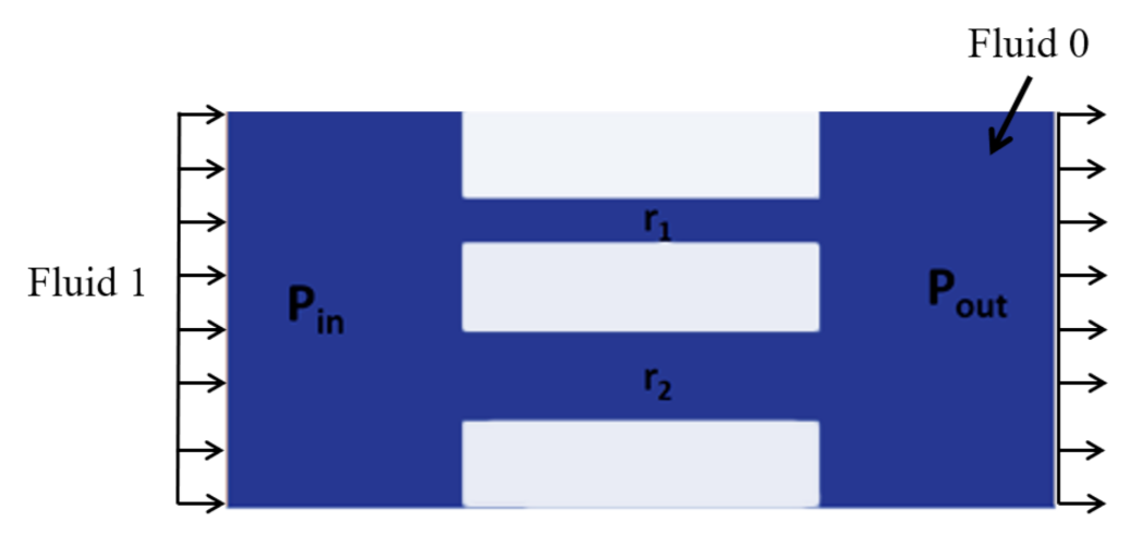
The validation of our model was carried out in consideration of a capillary pressure test with a known analytical solution. The test considered the injection of a gaseous phase from a plenum into two parallel passages (see Figure 2). The inlet and outlet boundary conditions were of uniform velocity and constant pressure, respectively, while the top and bottom walls were prescribed as on-grid bounce-back. The passages had different widths (r1 and r2) and, correspondingly, different capillary pressures (Pc1 and Pc2). Capillary pressure can be calculated by the Young–Laplace equation
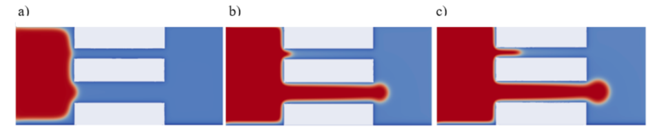
where is the surface tension. Then, the obtained values are compared to the pressure difference (Δp) at the inlet (pin) and the outlet (pout). Depending on the conditions present, the fluid can either enter or not enter the passages (note that passage 1 is narrower than passage 2). When Δp is less than Pc2, the gas cannot enter any of the passages, while if Δp is in the range from Pc1 to Pc2, the gaseous phase can only penetrate through passage 2. Finally, when Δp is larger than Pc1, the gas can fully penetrate through both passages.
The simulations were performed with contact angle θ = 70°, viscosity ratio D = 1 and a liquid–gas density ratio of 5, while r1 and r2 were chosen as 15 and 30, respectively. Three distinct pressure differences were simulated, namely Δp1 = 1.04 × 0−3, Δp2 = 2.13 × 10⁻³ and Δp3 = 4.3 × 10⁻³, where Pc1 and Pc2 are 2.51 × 10⁻³ and 1.25 × 10⁻³, correspondingly. All these quantities are in non-dimensional lattice units (lu).
The computational domain was discretized using 280 lattice units (lu) in the x-direction and 140 lu in the y-direction. The passages 1 and 2 are l00 lu in length by 15 lu-width and 30 lu-width, respectively. Figure 3 shows the excellent agreement between the numerical results and the expected flow behavior.
4. Results and Discussion
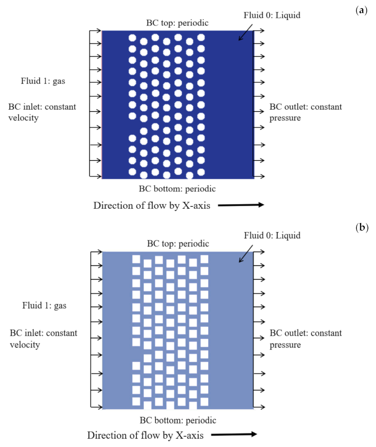
The schematic setup of the porous domain is shown in Figure 4a,b. Inlet and outlet boundary conditions are uniform velocity and constant pressure, respectively, while the top and bottom walls are prescribed as periodic boundary conditions. The computational domain has a size of 401 × 401 (lu2) and is filled with staggered columns of circular pores with a radius of 10 lu or square pores at 20 × 20 (lu2), separated by 10 lu. Each column of pores is spatially arranged uniformly with just a small perturbation (+1 and −1 lu) among contiguous pores to facilitate the break-up of flow symmetry during the simulation and resemble a more realistic flow behavior.
Additionally, one pore is removed from the 1st column to observe its effect on the fingering phenomenon. The uniform size and position of the pores in our study allows us a more precise control of the problem, which is different to what happens in experiments where pores often have different positions, pore sizes or variations in wettability. Initially, the porous medium is filled with the liquid phase, while the gaseous phase is introduced from the left to the right at a constant and uniform velocity. All simulations are conducted at a liquid–gas density ratio of 5, in order to have negligible spurious currents at gas-liquid interfaces [25].
The penetration of the gaseous phase is expected to depend on multiple dimensionless parameters, namely the capillary number (Ca), the viscosity ratio (D) and surface wettability. The capillary number Ca describes the relationship between viscous and interfacial forces:
where and are the average velocity and the dynamic viscosity of the gaseous phase, respectively. The viscosity ratio is defined as the ratio between the viscosity of the liquid and gaseous phases:
where is the dynamic viscosity of the liquid phase.
Furthermore, a common dimensionless time defined in Equation (16) is used in the comparison of gas penetration for cases with different injection velocity.
where is the total time-steps and H is the width of the domain.
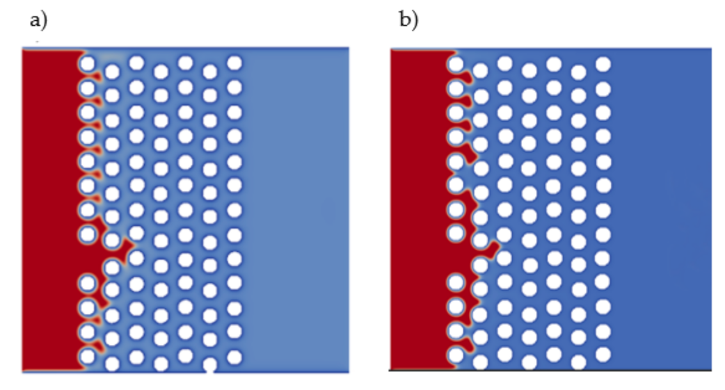
As a first stage in the modeling process, we performed a forcing scheme analysis to ensure its proper selection. For this purpose, the model with surface contact angle θ = 70°, Ca = 0.038 and circular pore geometry was selected. In this test, two different forcing schemes (namely velocity-shift and EDM) were analyzed under the same conditions at τ = 1. As can be seen from Figure 5, all simulations have approximately the same results, as previously proven in Section 2.2. Thus, further calculations at τ = 1 will be presented using the original velocity-shift forcing scheme. Nevertheless, the authors would like to suggest that for low-temperature and low-viscosity ratio fluid flow conditions not within the scope of this paper, the advantages of EDM over velocity-shift should be scrutinized, since the former might possess better numerical stability.
Multiple simulations were performed to identify the effect of Ca on the penetration of the gaseous phase into the porous media. Initially, the viscosity ratio was equal to 1 and the surface contact angle was set to θ = 70°, indicating a wettable condition. Three different capillary numbers were examined in this study, namely Ca1 = 0.038, Ca2 = 0.076 and Ca3 = 0.115. Different Ca can be obtained by varying velocity at the inlet boundary.
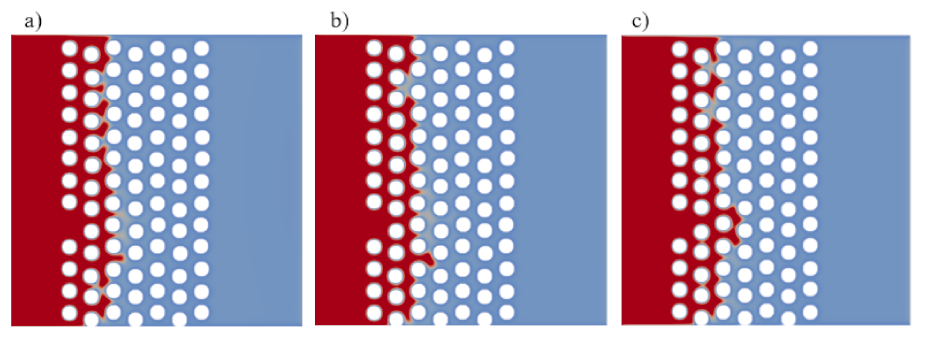
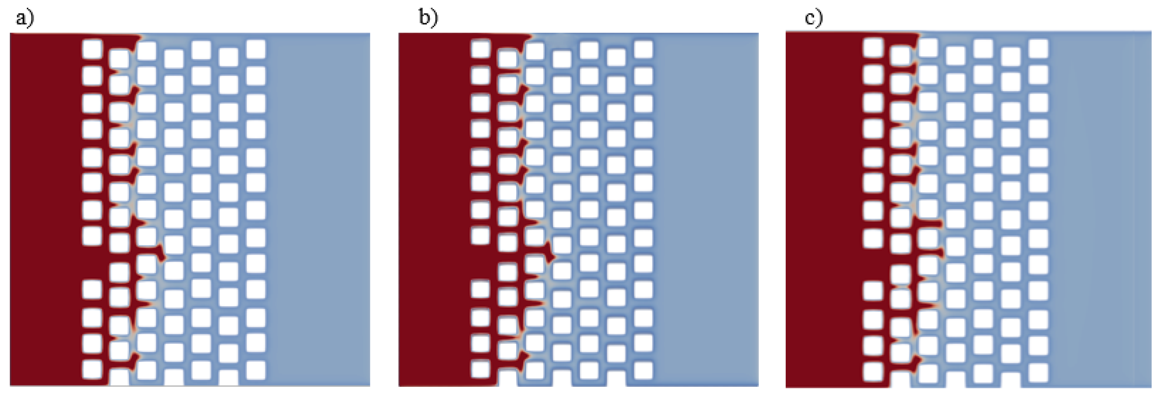
Figure 6 and Figure 7 illustrate the different penetration lengths at the common non-dimensional time = 0.175 at which the same amount of gas has been injected despite the injection velocity. Figure 6 and Figure 7 show that a larger Ca favors faster penetration of the gaseous phase into the porous media, as it was expected. Additionally, the fingering can be observed for each selected array of pore geometry near the entrance of the domain. Furthermore, at a lower Ca (Figure 6a and Figure 7a), it can be observed that the fingering favored the span-wise direction (with a larger pore throat) due to lower entry pressure, while it moved towards the stream-wise (front) faster with increasing Ca. Nevertheless, backward fingering, also known as capillary fingering, is hardly appreciated in our simulations, despite previous works observing that phenomenon being driven by the capillary force [28]. Lenormand et al. [36] also pointed out that capillary fingering may occur through a large pore throat in backward direction due to low entry pressure, but this backward-fingering is more noticeable for non-homogeneous porous media where the difference in pore throat between the cylinders is higher than that of the spacing used in the present investigation.
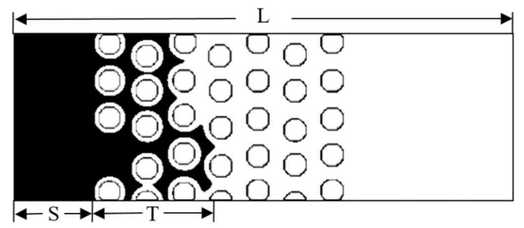
It is evident that, depending on pore geometry, the effective gas penetration, measured by length T (Figure 8), changes slightly, as shown in Table 3. Figure 8 illustrates the domain length (L), the slip distance (S) and the effective penetration length (T). In our case the slip distance is the same for all simulations.
Table 3 shows that, for low Ca, gas penetration is almost the same for both geometries, but as Ca increases, the penetration through the square-shaped pores is augmented significantly more than for the circular pores. We noted that extremely low Ca promotes the growth of spurious currents associated with numerical instabilities, consistent with findings by Raeini et al. [37].
Additionally, our results overcame the limitations found by Lenormand et al. [36], where it was stated that in a heterogeneous pore domain, a high Ca will force the fluid to occupy a limited fraction of the domain. Instead, our model has periodic boundary conditions, uniform size and uniform positioning of pores, removing that pitfall.
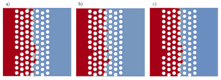
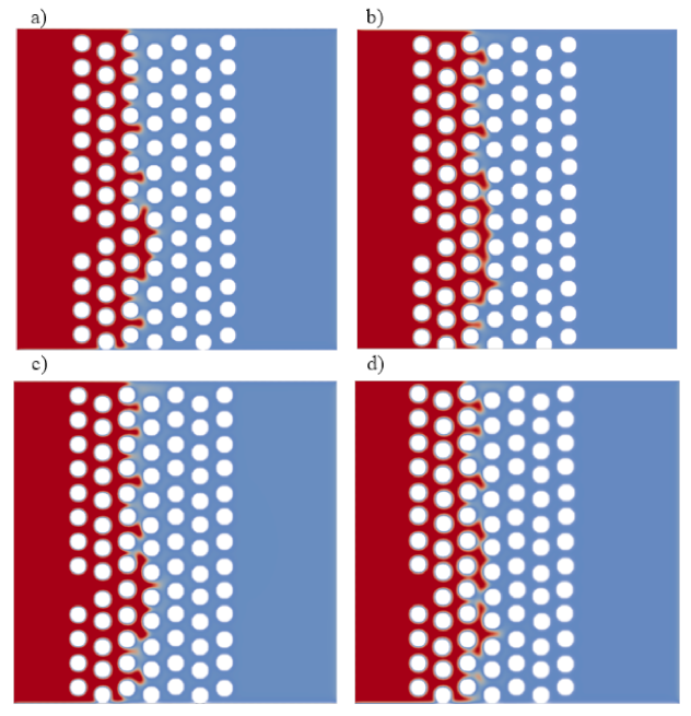
Furthermore, the effect of the viscosity ratio D is examined by varying gaseous phase viscosity while keeping the viscosity of the liquid phase constant. Additionally, Ca and θ are set as constant and equal to 0.038 and 70°, respectively. Figure 9 and Figure 10 show that increasing the viscosity ratio makes the gas injection more difficult and increases the time needed to displace the liquid phase out of the domain. The results corroborate previous studies, indicating that, at low D, the fingering narrows and spreads sideways faster, while it locally thickens when D increases [17]. Moreover, our results show the expected [27] easier front penetration at lower viscosity ratios, depicting how the intruding phase progresses faster in a finger-like manner as shown in Figure 9a and Figure 10a. Our results also corroborated that increasing the viscosity ratio favors a uniform frontal displacement (Figure 9c and Figure 10c). It should be noted that pore geometry affects the effective gas penetration length. According to Table 4, in the circular-shape pore domain, the gas penetration length is shorter than in the square-shape pore domain.
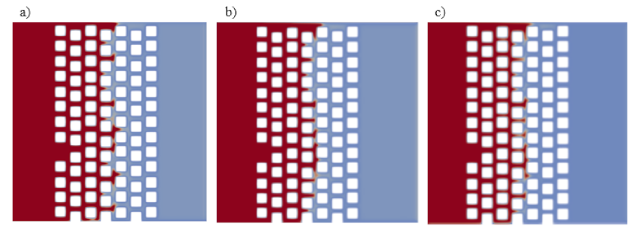
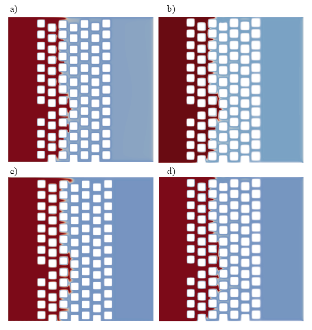
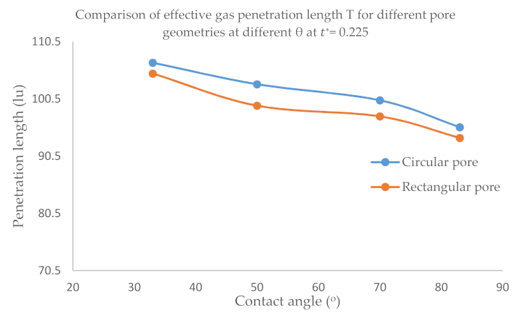
The effect of contact angle on gas penetration is investigated by changing the adhesion parameter between wall and fluid. As was previously discussed, depending on capillary pressure (Equation (13)), the gross evolution of the gaseous phase through the pores might be predicted. Consequently, the surface contact angle effectively affects the displacement of the gaseous phase into the liquid-filled porous domain. Previous studies [6,17] on porous media were done on a constant contact angle. Therefore, multiple simulations with various surface contact angles, namely = 83°, = 70°, = 50° and = 33° at fixed Ca, were carried out. Figure 9 demonstrates the evolution of the gaseous phase into the porous domain at = 0.225. All simulations were performed for wetting conditions, i.e., < 90°. Figure 9 shows how gas penetration length increases while the surface contact angle decreases, as was expected. However, the effective gas penetration in the circular-pore domain (Figure 11) is higher than that in the square-pore domain (Figure 12) due to the narrower inter-pore pas-sages (see Figure 13).
5. Conclusions
A multiphase LBM model was employed to study the influence of capillary number, viscosity ratio and surface contact angle on the hydrodynamics of gas penetration into a homogeneous 2D porous medium saturated with liquid. Previous studies [6,17,27,28] were done based on the phase-field (PF) method in a framework of a color-fluid multiphase LBM model with a density ratio of 1. In the present work, the Peng–Robinson EOS was successfully integrated into LBM in order to increase the stability of the model. As a result, P-R EOS enables the modeling of the gas penetration phenomenon with a liquid–gas density ratio of 5, resulting in negligible instabilities (i.e., spurious currents) at the interface. Additionally, the validity of the prescribed forcing scheme was assessed as one the main strategies to increase the stability of the model. It was found that at τ = 1 the velocity-shift and EDM forcing schemes performed similarly in terms of stability, and, therefore, the former was chosen to develop the whole set of simulations in porous media.
The numerical results demonstrated that increasing the capillary number (Ca) and surface wettability enhanced the effective gas penetration at constant viscosity ratio D, while an opposite effect is noticed when increasing D whilst maintaining constant Ca and wettability. Furthermore, the shape of the pores influences fingering length and effective gas penetration. In the present study, the effective gas penetration was higher in the square-pore domain than that in the circle-pore domain by approximately 10% and 4% for explored Ca,max and Dmin, respectively. Moreover, for the largest wettability explored in this study, the effective gas penetration in the square-pore domain was less than 3% than that in the circle-pore domain. Future work is planned to investigate gas–liquid penetration behavior in heterogeneous pore domains while increasing the viscosity ratio. What is more, in future study, we intend to use the EDM forcing scheme for better stability at low relaxation times.
Author Contributions
M.A.: developed the model set-up, simulations, and most of the analysis as lead author; B.K.: reviewed the model formulation and collaborated in the analysis of the results; E.M.: reviewed the model formulation and the literature review and collaborated in the analysis of the results; L.R.R.-S.: reviewed the model formulation and hypothesis statement and collaborated in the analysis of the results and overall content as supervisor. All authors have read and agreed to the published version of the manuscript.
Funding
This work was supported by Nazarbayev University MSc and PhD studentships of Magzhan Atykhan and Bagdagul Kabdenova (Dauyeshova), respectively, funded by the Ministry of Education and Science of the Republic of Kazakhstan. This work is also funded within the project NU Faculty Development Competitive Research Grants 2018, “Simulation of CO2 flow in porous media using Lattice Boltzmann Model”, #-090118FD5321.
Institutional Review Board Statement
Not applicable.
Informed Consent Statement
Not applicable.
Data Availability Statement
The data presented in this study are available in the displayed figures and tables within the article, but can also be obtained on request from the corresponding author within a reasonable time-frame.
Acknowledgments
The results reported in this study were obtained by using a modified version of the DL_MESO LBM package https://www.scd.stfc.ac.uk. The authors acknowledge M. Seaton for providing the original version of the code.
Conflicts of Interest
The authors declare no conflict of interest.
References
- Otomo, H.; Fan, H.; Li, Y.; Dressler, M.; Staroselsky, I.; Zhang, R.; Chen, H. Studies of accurate multi-component lattice Boltzmann models on benchmark cases required for engineering applications. J. Comput. Sci. 2016, 17, 334–339. [Google Scholar] [CrossRef] [Green Version]
- Lal, R. Carbon sequestration. Philos. Trans. R. Soc. B Biol. Sci. 2007, 363, 815–830. [Google Scholar] [CrossRef] [PubMed]
- Tsang, C.; Benson, S.M.; Kobelski, B.; Smith, R.E. Scientific considerations related to regulation development for CO2 sequestration in brine formations. Environ. Earth Sci. 2002, 42, 275–281. [Google Scholar] [CrossRef]
- Saxena, R.; Singh, V.K.; Kumar, E.A.; Kumar, E.A. Carbon Dioxide Capture and Sequestration by Adsorption on Activated Carbon. Energy Procedia 2014, 54, 320–329. [Google Scholar] [CrossRef] [Green Version]
- Taghilou, M.; Rahimian, M.H. Investigation of two-phase flow in porous media using lattice Boltzmann method. Comput. Math. Appl. 2014, 67, 424–436. [Google Scholar] [CrossRef]
- Liu, H.; Zhang, Y.; Valocchi, A.J. Lattice Boltzmann simulation of immiscible fluid displacement in porous media: Homogeneous versus heterogeneous pore network. Phys. Fluids 2015, 27, 052103. [Google Scholar] [CrossRef] [Green Version]
- Yang, J.; Boek, E.S. A comparison study of multi-component Lattice Boltzmann models for flow in porous media applications. Comput. Math. Appl. 2013, 65, 882–890. [Google Scholar] [CrossRef]
- Begum, R.; Basit, M.A. Lattice Boltzmann Method and its Applications to Fluid Flow Problems. Eur. J. Sci. Res. 2008, 22, 216–231. [Google Scholar]
- Gu, Q.; Liu, H.; Zhang, Y. Lattice Boltzmann Simulation of Immiscible Two-Phase Displacement in Two-Dimensional Berea Sandstone. Appl. Sci. 2018, 8, 1497. [Google Scholar] [CrossRef] [Green Version]
- Hirt, C.; Nichols, B. Volume of fluid (VOF) method for the dynamics of free boundaries. J. Comput. Phys. 1981, 39, 201–225. [Google Scholar] [CrossRef]
- Sussman, M.; Smereka, P.; Osher, S. A Level Set Approach for Computing Solutions to Incompressible Two-Phase Flow. J. Comput. Phys. 1994, 114, 146–159. [Google Scholar] [CrossRef]
- Jacqmin, D. Calculation of Two-Phase Navier–Stokes Flows Using Phase-Field Modeling. J. Comput. Phys. 1999, 155, 96–127. [Google Scholar] [CrossRef]
- Gunstensen, A.K.; Rothman, D.H.; Zaleski, S.; Zanetti, G. Lattice Boltzmann model of immiscible fluids. Phys. Rev. A 1991, 43, 4320–4327. [Google Scholar] [CrossRef]
- Dauyeshova, B.K.; Rojas-Solórzano, L.R.; Monaco, E. Numerical simulation of diffusion process in T-shaped micromixer using Shan-Chen Lattice Boltzmann Method. Comput. Fluids 2018, 167, 229–240. [Google Scholar] [CrossRef]
- Meakin, P.; Tartakovsky, A.M. Modeling and simulation of pore-scale multiphase fluid flow and reactive transport in fractured and porous media. Rev. Geophys. 2009, 47, RG3002. [Google Scholar] [CrossRef]
- Huang, H.; Krafczyk, M.; Lu, X. Forcing term in single-phase and Shan-Chen-type multiphase lattice Boltzmann models. Phys. Rev. E 2011, 84, 046710. [Google Scholar] [CrossRef] [Green Version]
- Liu, H.; Valocchi, A.J.; Werth, C.J.; Kang, Q.; Oostrom, M. Pore-scale simulation of liquid CO2 displacement of water using a two-phase lattice Boltzmann model. Adv. Water Resour. 2014, 73, 144–158. [Google Scholar] [CrossRef] [Green Version]
- Holtzman, R. Effects of Pore-Scale Disorder on Fluid Displacement in Partially-Wettable Porous Media. Sci. Rep. 2016, 6, 36221. [Google Scholar] [CrossRef]
- Hou, P.; Ju, Y.; Gao, F.; Wang, J.; He, J. Simulation and visualization of the displacement between CO2 and formation fluids at pore-scale levels and its application to the recovery of shale gas. Int. J. Coal Sci. Technol. 2016, 3, 351–369. [Google Scholar] [CrossRef] [Green Version]
- Isfahani, A.M.; Afrand, M. Experiment and Lattice Boltzmann numerical study on nanofluids flow in a micromodel as porous medium. Phys. E Low-Dimens. Syst. Nanostruct. 2017, 94, 15–21. [Google Scholar] [CrossRef]
- Tursynkhan, M.; Dauyeshova, B.; Adair, D.; Monaco, E.; Rojas-Solórzano, L. Simulation of Viscous Fingering in Microchannels With Hybrid-Patterned Surface Using Lattice Boltzmann Method. In Proceedings of the Volume 7: Fluids Engineering, ASME Meeting, Salt Lake City, UT, USA, 11–14 November 2019. [Google Scholar] [CrossRef]
- Fakhari, A.; Rahimian, M.H. Phase-field modeling by the method of lattice Boltzmann equations. Phys. Rev. E 2010, 81, 036707. [Google Scholar] [CrossRef] [PubMed]
- Inamuro, T.; Yokoyama, T.; Tanaka, K.; Taniguchi, M. An improved lattice Boltzmann method for incompressible two-phase flows with large density differences. Comput. Fluids 2016, 137, 55–69. [Google Scholar] [CrossRef]
- Lee, T.; Liu, L. Lattice Boltzmann simulations of micron-scale drop impact on dry surfaces. J. Comput. Phys. 2010, 229, 8045–8063. [Google Scholar] [CrossRef]
- Yuan, P.; Schaefer, L. Equations of state in a lattice Boltzmann model. Phys. Fluids 2006, 18, 042101. [Google Scholar] [CrossRef]
- Fakhari, A.; Li, Y.; Bolster, D.; Christensen, K.T. A phase-field lattice Boltzmann model for simulating multiphase flows in porous media: Application and comparison to experiments of CO2 sequestration at pore scale. Adv. Water Resour. 2018, 114, 119–134. [Google Scholar] [CrossRef]
- Liu, H.; Valocchi, A.; Kang, Q.; Werth, C.J. Pore-Scale Simulations of Gas Displacing Liquid in a Homogeneous Pore Network Using the Lattice Boltzmann Method. Transp. Porous Media 2013, 99, 555–580. [Google Scholar] [CrossRef]
- Zhao, H.; Ning, Z.; Kang, Q.; Chen, L.; Zhao, T. Relative permeability of two immiscible fluids flowing through porous media determined by lattice Boltzmann method. Int. Commun. Heat Mass Transf. 2017, 85, 53–61. [Google Scholar] [CrossRef]
- Li, Q.; Luo, K.H.; Li, X.J. Forcing scheme in pseudopotential lattice Boltzmann model for multiphase flows. Phys. Rev. E 2012, 86, 016709. [Google Scholar] [CrossRef] [Green Version]
- Kupershtokh, A.; Medvedev, D.; I Karpov, D. On equations of state in a lattice Boltzmann method. Comput. Math. Appl. 2009, 58, 965–974. [Google Scholar] [CrossRef] [Green Version]
- Chen, L.; Kang, Q.; Mu, Y.; Tong, Z.-X.; Tao, W.-Q. A critical review of the pseudopotential multiphase lattice Boltzmann model: Methods and applications. Int. J. Heat Mass Transf. 2014, 76, 210–236. [Google Scholar] [CrossRef]
- Shan, X.; Chen, H. Lattice Boltzmann model for simulating flows with multiple phases and components. Phys. Rev. E 1993, 47, 1815–1819. [Google Scholar] [CrossRef] [PubMed] [Green Version]
- Martys, N.S.; Chen, H. Simulation of multicomponent fluids in complex three-dimensional geometries by the lattice Boltzmann method. Phys. Rev. E 1996, 53, 743–750. [Google Scholar] [CrossRef] [PubMed]
- Huang, H.; Thorne, D.T.; Schaap, M.G.; Sukop, M.C. Proposed approximation for contact angles in Shan-and-Chen-type multicomponent multiphase lattice Boltzmann models. Phys. Rev. E 2007, 76, 066701. [Google Scholar] [CrossRef] [PubMed] [Green Version]
- Peng, D.-Y.; Robinson, D.B. A New Two-Constant Equation of State. Ind. Eng. Chem. Fundam. 1976, 15, 59–64. [Google Scholar] [CrossRef]
- Lenormand, R.; Touboul, E.; Zarcone, C. Numerical models and experiments on immiscible displacements in porous media. J. Fluid Mech. 1988, 189, 165–187. [Google Scholar] [CrossRef]
- Raeini, A.Q.; Bijeljic, B.; Blunt, M.J. Numerical Modelling of Sub-pore Scale Events in Two-Phase Flow through Porous Media. Transp. Porous Media 2013, 101, 191–213. [Google Scholar] [CrossRef]
Figure 1.
Comparison between the achievable lowest temperature with different forcing schemes at various relaxation times. Velocity-shift force scheme is presented in the graph as S-C.
Figure 1.
Comparison between the achievable lowest temperature with different forcing schemes at various relaxation times. Velocity-shift force scheme is presented in the graph as S-C.

Figure 2.
Initial setup for the capillary pressure test.

Figure 3.
Capillary pressure test results at different Δp: (a) Δp1 = 1.04 × 10⁻³; (b) Δp2 = 2.13 × 10⁻³; (c) Δp3 = 4.3 × 10⁻³.
Figure 3.
Capillary pressure test results at different Δp: (a) Δp1 = 1.04 × 10⁻³; (b) Δp2 = 2.13 × 10⁻³; (c) Δp3 = 4.3 × 10⁻³.

Figure 4.
(a) Initial and boundary conditions for the circular pore domain (white circles are pores with radius = 10 lu); (b) Initial and boundary conditions for the rectangular pore domain (white squares are pores with side = 20 lu).
Figure 4.
(a) Initial and boundary conditions for the circular pore domain (white circles are pores with radius = 10 lu); (b) Initial and boundary conditions for the rectangular pore domain (white squares are pores with side = 20 lu).

Figure 5.
Gaseous phase (red) penetration for circular pores at the 12,500th time-step, Ca = 0.038 with different forcing schemes: (a) velocity-shift; (b) EDM.
Figure 5.
Gaseous phase (red) penetration for circular pores at the 12,500th time-step, Ca = 0.038 with different forcing schemes: (a) velocity-shift; (b) EDM.

Figure 6.
Gaseous phase (red) penetration for circular pores at = 0.175 with different Ca: (a) Ca = 0.038; (b) Ca = 0.076; (c) Ca = 0.115.
Figure 6.
Gaseous phase (red) penetration for circular pores at = 0.175 with different Ca: (a) Ca = 0.038; (b) Ca = 0.076; (c) Ca = 0.115.

Figure 7.
Gaseous phase (red) penetration for rectangular pores at = 0.175 with different Ca: (a) Ca = 0.038; (b) Ca = 0.076; (c) Ca = 0.115.
Figure 7.
Gaseous phase (red) penetration for rectangular pores at = 0.175 with different Ca: (a) Ca = 0.038; (b) Ca = 0.076; (c) Ca = 0.115.

Figure 8.
Schematic illustration of gas penetration.

Figure 9.
Gaseous phase penetration for circular pores at = 0.275, Ca = 0.038, at: (a) D = 1; (b) D = 2; (c) D = 3.
Figure 9.
Gaseous phase penetration for circular pores at = 0.275, Ca = 0.038, at: (a) D = 1; (b) D = 2; (c) D = 3.

Figure 10.
Gaseous phase penetration for square pores at = 0.275, Ca = 0.038, at: (a) D = 1; (b) D = 2; (c) D = 3.
Figure 10.
Gaseous phase penetration for square pores at = 0.275, Ca = 0.038, at: (a) D = 1; (b) D = 2; (c) D = 3.

Figure 11.
Gaseous phase penetration at = 0.225 with fixed Ca = 0.038, D = 1, for various contact angles: (a) = 83°; (b) = 70°; (c) = 50°; (d) = 33°.
Figure 11.
Gaseous phase penetration at = 0.225 with fixed Ca = 0.038, D = 1, for various contact angles: (a) = 83°; (b) = 70°; (c) = 50°; (d) = 33°.

Figure 12.
Gaseous phase penetration for square pores at = 0.225 time-step with fixed Ca = 0.038, D = 1, for various contact angles: (a) = 83°; (b) = 70°; (c) = 50°; (d) = 33°.
Figure 12.
Gaseous phase penetration for square pores at = 0.225 time-step with fixed Ca = 0.038, D = 1, for various contact angles: (a) = 83°; (b) = 70°; (c) = 50°; (d) = 33°.

Figure 13.
Comparison of effective gas penetration length T for different pore geometries at different θ at = 0.225.
Figure 13.
Comparison of effective gas penetration length T for different pore geometries at different θ at = 0.225.


Table 1.
Weighting factors for D2Q9.
| I | wi |
|---|---|
| 0 | 4/9 |
| 1,3,5,7 | 1/9 |
| 2,4,6,8 | 1/36 |
Table 2.
Comparison of the maximum spurious currents for different forcing schemes.
| T/Tc | Velocity-Shift | EDM |
|---|---|---|
| 0.90 | 0.0693 | 0.0643 |
| 0.85 | 0.1126 | 0.1000 |
| 0.82 | 0.1399 | 0.1399 |
Table 3.
Comparison of effective penetration length T for different pore geometries at different Ca and = 0.175.
Table 3.
Comparison of effective penetration length T for different pore geometries at different Ca and = 0.175.
| Pore Geometry | Ca | T (lu) |
|---|---|---|
| Circular | 0.038 | 84.322 |
| Rectangular | 0.038 | 93.691 |
| Circular | 0.076 | 89.931 |
| Rectangular | 0.076 | 97.447 |
| Circular | 0.115 | 92.812 |
| Rectangular | 0.115 | 103.107 |
Table 4.
Comparison of effective penetration length T for different pore geometries at different D and = 0.275.
Table 4.
Comparison of effective penetration length T for different pore geometries at different D and = 0.275.
| Pore Geometry | D | T (lu) |
|---|---|---|
| Circular | 1 | 119.937 |
| Rectangular | 1 | 126.201 |
| Circular | 2 | 113.468 |
| Rectangular | 2 | 118.933 |
| Circular | 3 | 106.619 |
| Rectangular | 3 | 110.051 |
Publisher’s Note: MDPI stays neutral with regard to jurisdictional claims in published maps and institutional affiliations. |
© 2021 by the authors. Licensee MDPI, Basel, Switzerland. This article is an open access article distributed under the terms and conditions of the Creative Commons Attribution (CC BY) license (http://creativecommons.org/licenses/by/4.0/).
Share and Cite
MDPI and ACS Style
Atykhan, M.; Kabdenova, B.; Monaco, E.; Rojas-Solórzano, L.R. Modeling Immiscible Fluid Displacement in a Porous Medium Using Lattice Boltzmann Method. Fluids 2021, 6, 89. https://0-doi-org.brum.beds.ac.uk/10.3390/fluids6020089
AMA Style
Atykhan M, Kabdenova B, Monaco E, Rojas-Solórzano LR. Modeling Immiscible Fluid Displacement in a Porous Medium Using Lattice Boltzmann Method. Fluids. 2021; 6(2):89. https://0-doi-org.brum.beds.ac.uk/10.3390/fluids6020089
Chicago/Turabian StyleAtykhan, Magzhan, Bagdagul Kabdenova (Dauyeshova), Ernesto Monaco, and Luis R. Rojas-Solórzano. 2021. "Modeling Immiscible Fluid Displacement in a Porous Medium Using Lattice Boltzmann Method" Fluids 6, no. 2: 89. https://0-doi-org.brum.beds.ac.uk/10.3390/fluids6020089