
Thermal Conductivity of Ionic Liquids and IoNanofluids. Can Molecular Theory Help?


1
Centro de Química Estrutural, Faculdade de Ciências, Universidade de Lisboa, Campo Grande, 1749-016 Lisboa, Portugal
2
Chemical Engineering Department, Imperial College London, London SW7 2BY, UK
*
Author to whom correspondence should be addressed.
Fluids 2021, 6(3), 116; https://0-doi-org.brum.beds.ac.uk/10.3390/fluids6030116
Submission received: 5 February 2021
/
Revised: 25 February 2021
/
Accepted: 9 March 2021
/
Published: 12 March 2021
(This article belongs to the Special Issue Thermophysical Properties of Nanofluids - From Measurement to Interpretation)
Abstract
:Ionic liquids have been suggested as new engineering fluids, specifically in the area of heat transfer, and as alternatives to current biphenyl and diphenyl oxide, alkylated aromatics and dimethyl polysiloxane oils, which degrade above 200 °C, posing some environmental problems. Addition of nanoparticles to produce stable dispersions/gels of ionic liquids has proved to increase the thermal conductivity of the base ionic liquid, potentially contributing to better efficiency of heat transfer fluids. It is the purpose of this paper to analyze the prediction and estimation of the thermal conductivity of ionic liquids and IoNanofluids as a function of temperature, using the molecular theory of Bridgman and estimation methods previously developed for the base fluid. In addition, we consider methods that emphasize the importance of the interfacial area IL-NM in modelling the thermal conductivity enhancement. Results obtained show that it is not currently possible to predict or estimate the thermal conductivity of ionic liquids with an uncertainty commensurate with the best experimental values. The models of Maxwell and Hamilton are not capable of estimating the thermal conductivity enhancement of IoNanofluids, and it is clear that the Murshed, Leong and Yang model is not practical, if no additional information, either using imaging techniques at nanoscale or molecular dynamics simulations, is available.
1. Introduction
Ionic liquids appeared in the last two decades as one of the most promising categories of fluids for chemistry, chemical engineering, and medical applications. Composed of at least one cation and one anion, they are low temperature molten salts, capable of crystalizing at temperatures below room temperature and maintaining thermal and kinetic stability up to 550 K, restricted for most of them by their organic carbon content. From a molecular point of view, they are very interesting liquids because most of the well-known intra and intermolecular forces are present that, consequently, have a fundamental role in the structure and properties of these low temperature ionic melts.
For chemical processing operations, like extraction, separation, fluid movement, heat and mass transfer and reaction engineering, the properties of ionic liquids and of their mixtures with molecular and associating solvents are needed to design and operate the chemical plants. Additionally, their production at a reasonable price, needs optimization and scaling up of current laboratory type synthesis.
Owing to the large number of existing cations and anions, the number of combinations of them in ionic liquids is immense. To obtain the values of the thermophysical properties necessary for optimal process design, such as density, heat capacity, viscosity, and thermal conductivity, three alternatives exist: experimental measurements, predictive/estimation methods, and molecular simulation [1,2,3,4,5]. Being “target oriented” or “duty oriented” materials, the evaluation of their properties needs not only experimental measurements (very limited and time consuming), but theoretical developments and computer simulation, in order to develop sustainable and useful tools for project design, which we have carried through for molecular liquids. These arguments pave the way to predictive/estimation methods, a fundamental tool to be developed and incorporated in process design simulators. With the current knowledge of molecular simulation techniques, the understanding of ionic liquid structure and properties of ionic liquids and their mixtures is currently progressing, making ionic liquids a fundamental class of liquids for study and use in the next decades.
The concept of using dispersed nanomaterials (NM), particularly those that are carbon based, in ionic liquids [6], termed IoNanofluids, opened, a decade ago, the potential to use these nanofluids in several operations of heat transfer and storage, owing to the enhancement found in their thermal properties, especially their effective thermal conductivity. In addition to the molecular/ionic interactions in ionic liquids, it became interesting to study a new aspect, the interfacial area IL-NM, and its contribution to thermal conductivity enhancement.
It is the purpose of this paper to analyze the methods of prediction and estimation of the thermal conductivity of ionic liquids and IoNanofluids as a function of temperature. An attempt is made to clarify the use and misuse of terms in the literature. The term prediction has been widely used in the past to name methodologies that have totally different levels of theoretical or empirical support, while estimation is also used indiscriminately for purely based empirical schemes and for methods with some theoretical insight.
2. Concepts of Prediction and Estimation
The most recently available tool for the design of chemical process equipment and the simulation of its control and operation make use of very many features of process systems engineering implemented in extensive software codes that are closed to user examination. The evaluation of the thermophysical properties of the materials involved in the process are embedded within this software and are equally inaccessible. There is therefore an increased need for engineers using these tools to be aware of the limitations of the thermophysical data generated in this way. There is, equally an increased responsibility upon the scientists who provide this information to be clear about its pedigree and its likely reliability. Generally, such software packages offer choices between levels of sophistication and supposed accuracy for the various means of generating the requisite thermophysical property data which may include tables or correlations of experimental data, calculations on the basis of molecular theory and entirely empirical estimation procedures with no theoretical support. For the user a clear hierarchy for the nomenclature of all these processes is an invaluable guide to their likely reliability [7]. Some time ago we provided such a clear hierarchy of schemes for the generation of values for the transport properties of fluids [8]. However, since that time new fluids, such as ionic liquids have become much more common in the discourse around the chemical industry and that has been added to by the addition of nanofluids generally and IoNanofluids in particular. The scientists and engineers involved with these new materials have rather less familiarity with the background and implementation of such a hierarchy and there is therefore a danger of considerable confusion in both the literature and quality of schemes for the generation of thermophysical property data for such systems. We therefore wish to repeat our suggestions for a hierarchy in this new context.
First, we note that the reliance on accurate experimental data alone is not possible owing to the sheer numbers of materials and their mixtures that it would be necessary to study. Secondly, although it is perhaps desirable the application of rigorous molecular theory with known intermolecular potentials to calculate properties from first principles is possible only for systems no more complicated than methane gas in the dilute gaseous state. If both of these statements were true of simple fluids, they are even more valid for systems as complicated as ionic liquids and IoNanofluids. Certainly, in the latter case, as an example, the current enormous scatter of experimental measurements of the thermal conductivity of such fluids means that even this route is dangerous. As a consequence, all the alternative approaches we examined in our earlier work within the hierarchy are more prominent.
These alternatives, have been the object of pragmatic developments in the past by many authors, based on three basic approaches: approximate solutions of the fundamental theoretical equations, heuristic extensions of the theory (Van der Waals model, free volume theory) or on totally empirical information. Included in the latter group are group contribution methods, compiled in a series of excellent books, published since 1958 by McGraw-Hill, the latest being Poling et al. 5th edition [7]. It is still today a very helpful tool for all those that need, in the absence of accurate experimental data, to calculate the properties of pure and mixed compounds.
In the interest of clarity with set out in Figure 1 the scheme that was first proposed by Nieto Nieto de Castro and Wakeham [8] to characterize the pedigree of various schemes of generation of thermophysical property using their reliance upon molecular theory as the primary discriminant. This idea was further developed by Millat et al. [9], in chapter 3 of this reference. As a corollary, it has been demonstrated that the uncertainty of the generated thermophysical property data increases as the procedure departs more from a sound theoretical basis. The scheme relies entirely upon the correct interpretation of prediction, estimation, and correlation which are often used interchangeably and incorrectly in the literature. This is particularly true now in the field of ionic liquids whether they contain nanoparticles or not and justifies repetition of the correct description of these terms, established more than 30 years ago [8].
Prediction is defined as a scheme that has a rigorous theoretical framework and which requires as input information only physically meaningful quantities derived from a minimum set of accurate experiments or calculated from other fundamental sources. As mentioned above, the most effective substitute for direct measurement of the transport properties of fluids would be a complete, rigorous statistical-mechanical theory that enabled the calculation of the properties of the macroscopic ensemble of molecules from a knowledge of molecular properties and of the forces between the molecules (or ions). However, this approach is still limited to the calculation of the transport properties of dilute gases of simple molecules and their mixtures, using the kinetic theory of gases initiated by Boltzmann in 1872 and developed by Chapman-Enskog, with its extension to polyatomic species [9,10]. It is important to note that the same theory allows consistency tests between several transport properties and thereby the certification of state-of-art measurement instruments.
We designate as semi-theoretical predictions a subset of predictive schemes where a rigorous theory exists, which is devoid of approximations or contains approximations that are well characterized. Such a theory may lead to relationships between properties that enable one property that is hard to measure well from another for which is more easily measured. On example is the Eucken Factor for dilute gas properties [4]. Alternatively, the same approach allows an approximation at a molecular level in the theory to make calculations of properties tractable. The first example of this approach is the Mason and Monchick theory of the thermal conductivity of polyatomic gases [11,12]. Two further examples are afforded by the use of assumed intermolecular pair potential models for the evaluation of dilute gas viscosity data for polar gases [13] or the first density coefficient of viscosity and thermal conductivity of moderately dense non-polar gases [14,15,16].
When the rigor of theory is maintained, it is possible to develop less exact predictive schemes, which have considerable utility, even for low density phases. These predictive methods generally invoke a physical model of the interactions between the molecules in the system (homo and heteronuclear) and are designated by prediction methods and models. The best known of these schemes, departing the least from absolute rigor, is the Extended Law of Corresponding States—ELCS, based on the dimensional analysis of the Chapman-Enskog theory and its collision integrals, which considers that the spherical intermolecular pair potentials for among the species can be rendered conformal by a suitable choice of scaling parameters for energy ε and distance σ, developed by Kestin and co-workers in the 60′s [17], later extended to viscosity and binary diffusion of gaseous mixtures [18]. A detailed analysis, including extensions to thermal conductivity and viscosity of polyatomic gases, has been reported by Uribe and Mason [19]. The scheme can be applied to mixtures, predicting binary diffusion coefficients from viscosity data, to the viscosity of multicomponent gas mixtures, the thermal conductivity of multicomponent monoatomic gas mixtures, to the binary diffusion of multicomponent gas mixtures and other extensions to more complicated polyatomic molecules.
Estimation procedures are frequently thought of as those which are simply less accurate than the type of methods discussed above. However, we would like to define estimation in terms of the degree of departure from a sound theoretical basis, so that it is then possible to distinguish a hierarchy of levels of procedure and, consequently, identify our level of confidence in the scheme, with direct reflection in the uncertainty of the estimation. In that case, we can have four levels of confidence, namely: semi-theoretical estimation, approximate theoretical models, semi-empirical estimation, and empirical estimation.
In semi-theoretical estimation, the theory is maintained but some parameters within it have to be estimated without the benefit of accurate measurement. Self-evidently, the property data generated in this way are less accurate than if experimental data were used to estimate these parameters. On the other hand, the use of the correct theory guarantees that the results obtained retain structure which is essentially correct. As an example, we may cite the use of mixing laws to calculate the unlike pair interaction parameters from the like interaction parameters, in the application of the ELCS to mixtures [4,13]. A second class of theoretically inspired estimation methods occurs when a formal theory exists but its application to the interpretation of experimental data or estimation of properties is not possible, because of a combination of mathematical difficulty and inadequate knowledge of other necessary physical quantities. This is the case of the transport properties of simple liquids. The statistical mechanical theory developed by Bearman and Kirkwood (1958) [20] among others expresses their transport coefficients in terms of many particle distribution functions and intermolecular potentials. Since neither of these quantities are known, the theory cannot be applied at present (otherwise it would be classified as prediction).
Approximate theoretical models are designated as those where the procedures are founded upon an inexact theory. The theory may be inexact because simplifications were made in its development or because it is based upon a particular model. The classical example of this situation procedure in thermodynamics is the van der Waals equation of state and all those inspired in it, such as Redlich-Kwong, Peng and Robinson, Soave [7], etc., equations of state. In the field of transport properties of liquids, a similar type of procedure is the van der Waals model [21], based on the Enskog dense hard-sphere theory [22,23]. Another would be Bridgman’s model for the thermal conductivity of liquids, to which we shall give attention later [24], which assumed that liquid molecules are arranged in a cubic lattice and that energy is transferred from one lattice plane to the next at the speed at which sound travels through the fluid of interest (parallel to the original Maxwell elementary kinetic theory of gases). The model is simple and, to calculate the thermal conductivity of the fluid, data on the density, speed of sound and adiabatic compressibility (or the isothermal compressibility) are needed. Biddle et al. [25] applied this model to predict the thermal conductivity of supercooled water with a relative success. This model was recently applied to [C2mim][CH3SO3] [26], the calculated value for the polyatomic liquid being around 30% lower than the experimental value.
When an approximate theory is linked with behavior determined from experiment alone, other schemes evolve, herein designated by semi-empirical estimation. One such scheme is the extended corresponding states method of Hanley, Ely et al. [27,28,29,30,31,32,33] for non-polar fluids, refrigerants and molten salts, that converge in one of the most powerful software packages for thermodynamic and transport properties of fluids, REFPROP, now in version 10.0 [34]. A simplified, yet approximate, version of the exact theory is combined with dimensional analysis to lead to a corresponding-states procedure in terms of reduced, macroscopic variables, its implementation requiring a knowledge of the properties of a reference fluid. The empirical determination of the behavior of the reference substance provides the means to determine adjustable parameters (shape-factors) for a large number of other fluids from a limited set of information. The advantages of this kind of procedure lies in their generality and ability to make estimations over a wide range of states and classes of pure substances and mixtures. Extensions of such procedures by means of further empirical steps relating the requisite parameters of substances to critical point parameters and/or molecular structure then enable estimations of the transport properties of substances to be made for which no direct measurement exists.
The final subset of estimation methods is defined as that for which there is presently no theoretical justification, but which are based upon empirical observations of relationships between the experimental thermodynamic and transport properties of fluids and other macroscopic quantities for the same fluids. This type of estimation is designated by the term empirical estimation. They are by far the most numerous but, also, the most uncertain methods that exist. Most of the methods developed to calculate the thermophysical properties of gases at high densities and liquids belong to this subset of techniques [7,35]. An example is the representation of the reciprocal of liquid viscosity, the fluidity, as a function of its molar volume, proposed by Hildebrand (1971) [36], tested for several liquids, and extended to relations with other properties, like diffusion coefficients and electrolytic conduction.
All the methods based on group contributions, whereby properties of groups of atoms or molecular moieties are selected to contribute to the value of the property of the molecule fall into this category of scheme. In the case of thermal conductivity, the method of Koller et al. [37], based on an empirical relation between thermal conductivity and density, also applied in our recent publication [26] is a further example. No parameter is related to the molecular structure of the compound, and parameters are only obtained by n-functional fits to experimental data. Such correlations are formulated on a considerable body of data over a moderate temperature range and then applied universally to all fluids. Their success is not usually explained theoretically but calculated values are sometimes reasonable. However, procedures of this type have obvious deficiencies in terms of the accuracy of their estimates, are normally valid for a particular set of compounds and, furthermore, no indication is usually given of the possibility of extending to any number of components without further heuristic approximations. They are also obviously dependent on the quality of the experimental data that is used as the input. For some of the systems we examine here this is obviously an important fact. The sole advantage of such schemes lies in the fact that they may be applied to any chemical compound, independently of the molecular complexity of the system studied, although the risk of assuming using these values can be very high.
Unfortunately, the words prediction and estimation, are two terms used in current literature interchangeably, without making any reference to their origin and confidence. In particular, it is rare to have the word estimation included in the titles of papers, the authors (and reviewers) preferring the seemingly more erudite word prediction. We summarize in Figure 2 the relation between prediction, estimation, and uncertainty of property calculation schemes. The arrows also define the direction of each contribution (theory, experiment, confidence, universality, guess and specificity) for the magnitude of the expected uncertainty of the property calculation scheme. Values of uncertainties for molecular liquids are given only as an example. For ionic liquids they can, as we shall show below, easily be multiplied by a factor of three. They will also change from property to property.
A final comment is related with the word correlation. The correlation of different properties as a function of independent variable such as temperature or pressure can be merely empirical or developed with some theoretical insight. Fortunately, this last approach has been used in the last twenty years, for the thermophysical properties of selected commonly encountered fluids, over wide ranges of temperature and pressure. These correlations need a trustworthy EOS, and many examples can be seen in the Journal of Physical and Chemical Reference Data. However, in the literature, the use of correlation is very often restricted to a narrow range of temperature (and sometimes pressure) and to a single properties, obtained experimentally. Such correlations cannot generally be use outside of the range of conditions for which there are data and are therefore of limited utility [9].
3. The Case of Ionic Liquids—Tools for Prediction and Estimation of Thermophysical Properties
The nature of the low temperature melting salts is governed by a complex combination of Coulombic, hydrogen bonding and Van der Waals interactions of their ions. In simple salts the interactions are controlled by long-range Coulomb forces between the net charges of the ions. In addition, with ions composed mostly by organic moieties, their bulky size and asymmetric charge distribution softens the Coulombic forces and generates highly directional interactions of shorter range (see Table 1 for a short list of monovalent cations and anions present in ionic liquids). Consequently, the interaction potential depends not only on the distance r of the ions, but on a set of angles Ω for their mutual orientation, causing non-spherical interactions, the case being worse when hydrogen bonding is present. These forces give rise to several phenomena, like conformational equilibria in cations, the formation of ion pairs and large ion clusters in the liquid phase, which affect the dynamics of the molecule movement, especially important for transport properties, like viscosity, thermal conductivity, electrical conductivity and ion-diffusion.
The number of combinations of cations and anions is immense, ~1018, and the structure of the cations (usually non-symmetric) and anions varies very much. Therefore, charge distributions are not simple to calculate, and all these facts complicate modelling or theory development. The packing of molecules in ionic liquids is similar to a crystal in the first 2–3 coordination spheres, with a well-defined peak cation-anion (well-defined peaks at r ~ 0.4 and 0.8 nm—distance of the imidazolium ring to chlorine ion), and a cation-cation ill-defined peak at r ~ 0.92 nm as observed by Hardacre et al. [38] with neutron and X-ray diffraction studies of [dmim][Cl], which melts at 401 K and gives a relatively simple structure of an ionic liquid (Figure 3a).
Canongia Lopes and Padua in 2006 [39], using computer simulation, showed that an all-atom force field predicted that pure ionic liquids of the 1-alkyl-3-methylimidazolium family [Cnmim][PF6] (n = 2 to 12), have structuring of their liquid phases in a manner that is analogous to microphase separation between polar and nonpolar domains, as shown in Figure 3b for n = 2 and 6. It was observed that the polar domain has the structure of a three-dimensional network of ionic channels, whereas the non-polar domain is arranged as a dispersed microphase for 1-ethyl-3-methylimidazolium ILs and as a continuous one for longer side-chains, such as hexyl, octyl, or dodecyl; the butyl side-chain marks the onset of the transition from one type of structure to the other.
Can we use the methodology described in Section 2 for Ionic Liquids? Generalizations are impossible owing to our limited current understanding at a nanoscale, of the existing intermolecular forces and the supporting theories, it is extremely difficult to develop theoretically based predictive schemes. Even if we now understand the structure of IL’s in the liquid state (mostly with imidazolium rings) we cannot yet calculate properties, except by modelling the interactions and performing molecular dynamics experiments.
A series of estimation methods that enable the calculation of transport properties, therefore have to be developed, based on:
- (a)
- approximate theoretical models (e.g., Bridgman model),
- (b)
- heuristic extensions of the theory (e.g., Van der Waals model, free volume theory),
- (c)
- totally empirical information, such as the behavior of a given property for a group of structural similar compounds (e.g., group contribution methods), or empirical relations between thermophysical properties (e.g., Koller method).
A brief description of each approach is described below, with especial emphasis on the Bridgman, Van der Waals and Koller methods.
3.1. Bridgman Model
As explained above, Bridgman [24] assumed that liquid molecules are arranged in a cubic lattice and that energy is transferred from one lattice plane to the next at the speed at which sound travels through the fluid of interest. The cubic lattice was chosen to have a center-to-center spacing given by (v*) 1/3, v* being the volume per molecule (the molecular volume). The distance travelled between two consecutive collisions and so the distance between neighboring planes, is equal to the center-to-center spacing.
The development is based on a reinterpretation of the kinetic theory of gases (rigid spheres), and can be found on the book by Hirschfelder, Curtiss and Bird [40], leading to:
where λ is the thermal conductivity of the liquid; kB is the Boltzmann constant; u the speed of sound in the limit of zero frequency. The numerical coefficient was initially 3 but was empirically modified to 2.8 to secure better agreement with experimental data. Using the thermodynamic relation:
in the absence of speed of sound data, where ρ is the density and κS the adiabatic compressibility, we obtain:
Because the adiabatic compressibility is very difficult to obtain, the method uses Eyring’s modification [34], as described by Biddle et al. [25]:
where κT the isothermal compressibility, a quantity that is much simpler to obtain.
This equation is limited to densities well above the critical density because it assumes that each molecule oscillates in a “cage” formed by its nearest neighbours. It was derived for monatomic liquids, for which CV = 3 kB/m, m being the mass of a molecule, which is less than the heat capacities of polyatomic liquids. Therefore, Equation (4) underestimates the calculated value of thermal conductivity and we shall discuss this point in Section 5.1. This model is quite unrealistic for simple fluids where computer simulation does not support the notion of a cage of molecules with occasional long-distance jumps, but the structure within IL’s means that it may be more appropriate for them. This model was applied for the first time by Lozano-Martín et al. (2020) [26] for the ionic liquid [C2mim][CH3SO3] and will be pursued in this paper for other ionic liquids.
3.2. Van der Waals Model
The application of a hard-sphere scheme to the estimation of the viscosity and thermal conductivity of ionic liquids has been reported by Gaciño et al. in 2014 [41], with success. A database of 461 viscosity and 170 thermal-conductivity measurements for 19 ionic liquids was used. Expanded uncertainty at the 95% confidence level was 4.6% and 6.3%. According to the model, the reduced thermal conductivity, λ*, is defined in Equation (5) as:
This reduced thermal conductivity is a function of the reduced molar volume Vr = V/V0, where V is the molar volume and V0 is a characteristic molar volume of the liquid, weakly dependent on temperature (originally considered as a close-packed volume). M represents the molecular mass and R the universal gas constant. The parameter Rλ, introduced for polyatomic molecules, accounts for deviations from the behavior of smooth hard spheres [23]. Because the viscosity is more sensitive to the characteristic molar volume, V0 was obtained from viscosity data. The method uses a correlation of the experimental data available for the ionic liquids considered, with coefficients that are listed in Tables 1 and 7 of reference [41]. The method is limited to systems for which density data for the ionic liquids exist, but this is not a very serious limitation, because it is the most commonly available thermophysical property [42]. Moreover, if the thermal-conductivity roughness factor, Rλ, is allowed to be temperature dependent, then the average absolute deviation of all ionic liquid thermal conductivity data can be reduced to 0.91% for the thermal conductivity, and the expanded uncertainty at the 95% confidence level to 1.82%, which is a very good result. Figure 4 shows the deviation of the experimental data from the proposed correlating scheme, as a function of the reduced molar volume. If this scheme is used for estimating the thermal conductivity of the 19 ionic liquids used in the development, a maximum error of ±4% is found. It is worth pointing out that deviations of this size are smaller than the likely experimental uncertainty in the transport property measurements, particularly for the thermal conductivity but also the viscosity.
3.3. Koller Method
From among the purely empirical methods, based on relations between other thermophysical properties and thermal conductivity, we can select the Mohanty relationship, based on the Andrade theory for liquid viscosity [43] and the Bridgman theory for molecular collisions described above. Mohanty [44] proposed a very simple relationship between thermal conductivity and viscosity, Mλ/η = Const, with the constant having an average value of 10.8 for organic liquids at room temperature. This relationship was explored by Tomida et al. [45], for [C4mim][PF6], [C6mim][PF6], and [C8mim][PF6] from 294 to 335 K at pressures up to 20 MPa. They arrived at the conclusion that the Mohanty constant was, in practice, a function of molecular mass for the ionic liquids, and obtained Equation (6):
However, in order to maintain agreement with the data for n-alkanes, which are much less viscous, it was necessary to multiply by 2 the value of the molecular mass of the ionic liquids, i.e., M’ = 2 M, which is most unsatisfactory from a fundamental perspective.
Fröba et al. [46] discussed Equation (6) and found that it could not estimate correctly the thermal conductivities of a series of [C2mim]-based ionic liquids (ILs) having the anions [(CF3SO2)2N], [CH3OCO], [N(CN)2], [C(CN)3], [C1OHPO2], [C2OSO3] or [C8OSO3], and in addition for ILs with the [(CF3SO2)2N]− anion having the cations [C6mim], [OMA], or [BBIM]. They therefore proposed a relation between thermal conductivity, density, and molecular mass, giving Equation (7):
In this equation the parameters A and B where obtained by least-squares fitting of all the experimental results existing at the time, at a temperature of 293.15 K and atmospheric pressure. For this case the coefficients in Equation (7) are A = 1.244 and B = 18.84, when all quantities expressed in SI units. A standard percentage deviation of 7.8% (15.6% at 95% confidence level) was found. This equation was also adapted by Ferreira et al. [47] for phosphonium and ammonium cations, using values of A = 1.36 and B = 8.533, with standard percentage deviation of 4% (8% at 95% confidence level). Figure 5 shows the deviations for the thermal conductivity of [P66614]+ ionic liquids with different anions, Ferreira et al.[47], Ge et al. [48] and França et al. [49]. It can be seen, that apart from bis(2,4,4-trimethylpentyl)phosphinate, already noted by Ferreira et al. [47], the deviations for the other ionic liquids vary between −5% and +15%. However, these results show a definite trend with temperature, probably because the methods, such as that of Fröba et al. [46] equation, do not account for different temperature variation of density and thermal conductivity.
The Erlangen group tried to resolve this situation, by introducing a correction to accommodate the temperature variation, reported by Koller et al. [37]. Their relation based upon the existing thermal conductivity data for 53 ILs, is expressed by Equation (8):
where λ is the calculated thermal conductivity, ρ is the density and M the molar mass, all expressed in SI units. The parameters they report are A = 0.0960, B = 21.43, C = 0.826 and Tref = 293.15 K, with quantities expressed in SI units. This equation has a claimed AARD (average absolute relative deviation) of 6.3% (12.6% at a 95% confidence level) and also includes many ammonium and phosphonium liquids, the object of the analysis of Ferreira et al. [47]. These results are very good, as most of the experimental data used in the development have uncertainties of this order of magnitude. Deviations for compounds not used in the development, like [C2mim][CH3SO3] [26], underestimated the thermal conductivity 8% at 293 K and 14% at 343 K, an interesting result.
3.4. Group Contribution Methods
The discussion of group contribution methods will be brief, because they will not be applied in this paper. Many of them involve other thermophysical properties, such as the isobaric heat capacity CP.
Gardas and Coutinho developed group contribution methods for estimating the thermophysical and transport properties of ILs for viscosity, electrical conductivity, thermal conductivity, refractive index, isobaric expansivity and isothermal compressibility [50]. The parameters of the group contribution methods were determined for imidazolium-, pyridinium-, pyrrolidinium-, piperidinium-, phosphonium-, and ammonium-based ionic liquids. For thermal conductivity 16 IL’s, the average absolute relative deviation, AARD, was found to be 1.06%, with deviations of ±2–4%, for lower and higher thermal conductivities, a very good result. Group contributions were calculated for a limited number of cations, anions and methylene and methyl groups, owing to the scarcity of thermal conductivity data at the time of publication. In spite of its simplicity, the method has no capacity to estimate the properties for fluids with cations and anions not in the base set, as for example for DCA or P66614 ions.
Wu et al. [51] adopted a new equation, similar in form to Reidel equation [52], to correlate the thermal conductivity of ionic liquids, based on reduced temperature, with boiling and critical temperatures estimated from Valderama et al. formulas [53]. However, these parameters are obtained with high uncertainty owing to the small vapor pressure of ionic liquids, which decompose before reaching their vapor-liquid critical point. 36 ionic liquids were covered. Group contributions were optimized for groups with rings and without rings, and the reader is referred to Table 1 of reference [51]. For the ionic liquids studied, the overall AARD was found to be 1.66% (3.3% at 95% confidence level), with a maximum deviation less than 11 (22%). Again, this application is limited to IL’s where the groups constituting the anion and cation were evaluated by the authors.
The method of Wu et al. [51] was optimized by Oster et al. [54], by using DFT calculations to optimize charge distribution and structural contributions, and using recent data for new ionic liquids, a total of 55. The model developed used a novel approach to include the impact of cation core atom on the structure and physical properties of the ionic liquids. The overall AARD, for all data sets used is 1.66% (3.3% at a 95% confidence level), much better than the average uncertainty of used experimental data, with maximum AARD of 7.16% for 1,3-dibutylimidazolium bis[(trifluoromethyl)sulfonyl]imide, [C4C4im][(CF3SO2)2N]. Tables 2 and 3 of reference [54] show the ionic liquids covered and the new parameters for the Wu model equation.
4. The Case of IoNanofluids—Tools for Calculating Thermal Conductivity Enhancement
Dispersions of nanoparticles in several fluids were firstly studied by Yang and Maa [55] in 1984 in their boiling heat transfer study and Masuda et al. [56] in studying the viscosity and the effective thermal conductivity of Al2O3, SiO2 and TiO2 (anatase) ultra-fine particles (13, 12 and 27 nm, respectively) dispersed in water. This effective thermal conductivity is not a true thermal conductivity because the systems studied are two-phase at least, and some authors designate it as apparent thermal conductivity. However, these authors identified what seemed to be one of the most sensitive phenomena in heat transfer in the last century, the enhancement of thermal conductivity of the media with respect to the original base fluid. The impact of nanofluids in current science and technology was catalysed by the work of Choi et al. using classical heat transfer fluids, like water, ethylene glycol and engine oil [57], whose results (now shown to be very substantial overestimates), contributed however to a revolution of research on heat transfer fluids. The use of composites of carbon nanomaterials in ionic liquids, namely multi-walled carbon nanotubes (MWCNTs) was first reported by Aida et al. [58] who mixed ionic liquids with carbon nanotubes (CNTs), forming highly viscous gels, called Bucky Gels, a tribute to the architect Richard Buckminster Fuller (Bucky), famous for his geodesic domes. These nanosystems are now designated IoNanofluids [6], a stable dispersion of nanomaterials in ionic liquids. Those and related systems have a number of applications including in new materials, processes, and electronic or electrochemical devices. Ionic liquids supported in gels are relevant as membranes for separations [59], can be designed as solvents for exfoliation [60,61] of carbon nanomaterials, leading to stable suspensions and new ways to functionalize or manipulate those nanomaterials, or new composite phases. Applications of lower viscosity IoNanofluids are today widely contemplated. The interface between ionic liquids and carbon nanomaterials is relevant in many contexts, for example in the development of better electrolytic supercapacitors [62], by design of the organic electrolyte or by the electrode nanoporous carbon material [63], the use of carbon nanofibers in IL-based catalytic beds to improve the specific surface area [64] or the performance enhancement of dye-sensitized solar cells with IL electrolytes using carbon dots [65].
Dispersions of nanomaterials in ionic liquids have already been studied by our group in different systems [6,66,67,68,69,70,71,72,73,74,75,76,77], both from experimental and theoretical points of view; the systems have involved MWCNTs, melanin (natural nanomaterial [66]) and graphene. The thermophysical properties of the IoNanofluids were measured and an interpretation of the unexpected enhancement in thermal conductivity was explained with regard to the effect of the particle surface chemistry and of the interphase particle/fluid structure.
In this paper we will restrict the analysis to the systems based on dispersions of MWCNTs in ionic liquids. In our first paper [6], the Maxwell model [77] and the Leong et al. [78,79] models for spherical nanoparticles were used to explain the thermal conductivity enhancement in several IoNanofluids. However, in the second of these models, calculations are strongly affected by the values assumed for the thermal conductivity of the interfacial layer and for its thickness [49,69,70,71]. As an example, for an interfacial thickness of 2 nm, the model of Leong et al. can only be applied to systems with an enhancement higher than 20%, which usually happens only for high volumetric nanoparticle fractions (>3%). In our system with [C4mim][(C2F5)3PF3][76], a very small value of enhancement (6.2%) was found.
Figure 6 summarizes the average thermal conductivity enhancements found for all the IoNanofluids studied in our laboratory, between 293 and 353 K, for a concentration of 1% (w/w) of MWCNT’s. Values vary between 2 and 12%, which are rather modest effects; and no dependence on molecular structure of the cations or anions can be identified.
For example, if we select just the effective thermal conductivity of liquids with the same cation, [C4mim]+, and compare them with the values of the thermal conductivity of the base fluid, the result is displayed in Figure 7.
The order for the enhancement decreases as shown in the Figure 7a, while the thermal conductivity of the corresponding ionic liquid varies randomly (7b). In Figure 8 we show the variation of the thermal conductivity enhancement with the same cation, [C2mim]+, (a) and with the same anion, [(CF3SO2)2N]−, (b). The ion size does not seem to have a specific effect, as was discussed for thermal conductivity dependence of the same liquids [77]. The sequence obtained for the thermal conductivity was: [(CN)2N]− > [C(CN)3]− ≈ [SCN]− > [BF4]− > [PF6]− > [CF3SO3]− > [(CF3SO2)2N]− > [(C2F5)3PF3]−. A bulky ion like [(C2F5)3PF3]−, which is much less mobile, seems to contribute to a very low thermal conductivity. Cyano-anions introduce a much higher value for the thermal conductivity, and a stronger dependence on temperature. The thermal conductivity of [C4mim][BF4], with the smallest anion, is high, but lower than that of cyano-compounds, especially at the lower temperatures. For the other ILs the value of the thermal conductivity increases with decrease of the anion size. Smaller anions have, in principle, better mobility, increasing the ionic interactions and consequently promoting more heat paths.
It seems that the mechanism of thermal energy transfer in the IoNanofluid, reflected macroscopically in the thermal conductivity, is not very dependent on the properties of the base ionic liquid. However, it has been argued that it may depend on the interactions between the ionic liquid moieties and the surface of the nanomaterial (interface particle/fluid) and on the surface chemistry involved. This result was a conclusion of our publication [49], as well as the Belfast/Manchester group [80] and the Katowice group [81]. Other possible contributions to the thermal conductivity enhancement in IoNanofluids containing MWCNTs were not considered.
França et al. [75] showed that, for the atoms of ionic liquids and carbon nanomaterials interacting among themselves, attraction is stronger for cations (than for anions) above and below the π-system of the nanomaterials, whereas anions show stronger attraction for the hydrogenated edges. The ordering of ions around and inside (7, 7) and (10, 10) single-walled nanotubes, and near a stack of graphene sheets, was analysed in terms of density distribution functions. The anions, as well as cations, were found in the first interfacial layer interacting with the carbon nanomaterials, which is surprising given the interaction potential surfaces used. The thermal conductivity of the ionic liquids and of composite systems containing one nanotube or one graphene stack in suspension was calculated using non-equilibrium molecular dynamics. In the composite systems containing the nanotube there is an enhancement of the overall thermal conductivity, with calculated values comparing well with experiments on nanotube suspensions, namely in terms of the order of the different ionic liquids.
A very detailed review of the existing models to calculate the effective thermal conductivity of solid particle suspensions (λeff), like nanofluids, particularly with CNT’s, can be seen in references [82,83,84,85,86], and no detailed discussion will be performed here. Most of them have a mechanistic base, regarding the dispersion of well-dispersed solid particles in a continuous medium, originating from the pioneering work of Maxwell [77] analogous electrical problem. This treatment was valid only for spherical particles. Hamilton and Crosser [86], modified it for non-spherical particles and shape factors for particles, such as cylinders, were introduced. The latter model shows that the enhancement in thermal conductivity for non-spherical particles is higher than for spherical particles. These classical models were found to be unable to predict and explain the experimental thermal conductivity of nanofluids, namely the dependence on temperature and particle volume fraction [81,84,87]. Despite a large research effort devoted in the last decade to identify the mechanisms and to develop theoretical models for heat transfer in nanofluids, current knowledge on the real heat transfer mechanisms is scarce and controversial [49,84].
Generally, additional mechanisms have been proposed to explain, at least qualitatively, the observed enhancement of the effective thermal conductivity of nanofluids beyond that predicted by these classical models. These additional mechanisms include Brownian motion of nanoparticles (for spherical shape), interfacial nanolayer at the surface of nanoparticle/base fluid interface, and nanoparticle clustering or aggregation. These mechanisms are well discussed in the literature [83,84,88] and will not be elaborated further here. Among these mechanisms, the interfacial nanolayer has been suggested as the major factor behind the increase in the effective thermal conductivity of nanofluids [79]. The liquid molecules near the particle surface interact and/or are absorbed at the nanoparticle surface creating a layered structure, which shows characteristics of an organized “solid” like system [80,81,82,83,84,85,88,89]. Figure 9 shows a schematic drawing of this concept, and its realization using molecular dynamics by João França et al. (2017) [75,90], for a simulation with SWCNT + [C4mim][C(CN)3], at 363 K. This observation lent credibility to our previous understanding of the feasibility of the model of Leong et al. [73,79] and similar models, that an interface exists in a CNT-IL system with a temperature jump, at the surface of the tube affecting the heat transfer mechanism. The existence of the layer was confirmed by its application to ionic liquids, not only for SWCNT, but also for graphene. Within the models of Leong et al. it is then possible to use this theoretical development for the calculation of the thermal conductivity of IoNanofluid with carbon tubes, once we know, experimentally or by using empirical estimation techniques, the thermal conductivity of the base ionic liquid, as well as the properties of the interfacial layer, specifically its thickness and thermal conductivity. Of course, the entire process is limited by the uncertainty of the experimental values of the thermal conductivity used.
A brief description of the main equations for the models used in this study is necessary. The Maxwell model [78] predicts the effective thermal conductivity of liquid-solid suspensions for spherical particles and results in Equation (9):
where λp and λIL are, respectively, the thermal conductivity of the nanoparticles and of the base ionic liquid, λINF is the effective thermal conductivity of the IoNanofluid, and ϕp is the volume fraction of the nanoparticles in the IoNanofluid. Hamilton and Crosser [86] modified Maxwell’s model for both spherical and non-spherical particles by applying a shape factor n, that considers the shape of the dispersed particles. This shape factor is a function of the sphericity, used previously to characterize the shape for particles falling through liquids [91]. Sphericity, ψ, is defined as the ratio of the surface area of a sphere with volume equal to that of the nanoparticle, to the surface area of the nanoparticle. The Hamilton and Crosser model results in Equation (10):
As mentioned above, this model reveals an increase in thermal conductivity for non-spherical particles (with the same volume fraction) higher than that for spherical particles. This expression reduces to the Maxwell model for spherical particles (n = 1).
Leong et al. [78,79] developed two models by considering the effects of particle size, its concentration, and added an interfacial nanolayer, for nanofluids containing spherical and cylindrical nanoparticles. Their model (MLY) [92] for nanofluids containing cylindrical/tube nanoparticles for calculating the effective thermal conductivity of our IoNanofluid, λINF has the form:
And defining F as:
we obtain for the thermal conductivity enhancement, ,
where λp and λIL are the thermal conductivity of the nanoparticles and of the base ionic liquid, ϕp is the volume fraction of the nanoparticles in the IoNanofluid, ω = λlr/λIL, γ = 1 + h/rp, and γ1 = 1 + h/(2rp), h and λlr are the thickness and the thermal conductivity of interfacial nanolayer, respectively, and rp is the radius of the nanoparticle.
The values of λp and λIL can be obtained from the literature (or estimated, if necessary), if the nanoparticles used are well characterized. However, values of h and λlr significantly influence the value calculated for the thermal conductivity of the IoNanofluid. The order and orientation of fluid molecules absorbed on the nanoparticle surface seems to lead to a value for the thermal conductivity of the nanolayer which is intermediate between that of the solid and the base fluid; i.e., λIL < λlr < λp. For CNT’s, their thermal conductivity is of the order of 3000 W·m−1·K−1, as measured using a micro fabricated suspended device [93], a factor of 20,000 greater than the average thermal conductivity of an ionic liquid. However, this value is controversial, as many authors, with different methods, arrived at values for the thermal conductivity of individual or bundle single walled and MWCNTs in the range of from 20 to 6000 W·m−1·K−1 [94,95,96,97]. Our MWCNTs were furnished at no cost by Bayer (Baytubes® C150HP, CAS Nr. 308068-56-6), with lengths varying from 1–10 µm, with an average outside diameter of 13–16 nm, a bulk density of 140–230 kg·m−3 and a purity ≥ 99%. The tubes are entangled and look similar to chains in polymers [98], as shown in Figure 10. In the absence of an experimental measurement, we estimated a value between 2000–3000 W·m−1·K−1 for this type of MWCNTs in our previous publications, which is consistent with that used by others [80,81].
5. Results
In this section we examine the performance of the schemes proposed for the estimation of the thermal conductivity of nanofluids and IoNanofluids.
5.1. Thermal Conductivity of Ionic Liquids
As mentioned in Section 3.1, the Bridgman model makes the thermal conductivity only dependent on the density and on the speed of sound of the ionic liquid (Equation (1)). This model was applied to all the ionic liquids studied, for which speed of sound was available (no data for [C2mim][(CN)2N] and [C4mim][C(CN)3]) or at some higher temperatures for other IL’s (eg. [C2mim][SCN] at temperatures greater than 323 K). As mentioned in our application for [C2mim][CH3SO3] [26], the Bridgman model underestimates the thermal conductivity of this ionic liquid. Figure 11 displays λexp as a function of λcalc, and many points are underestimated by more than 50% (e.g., [C6mim][(CF3SO2)2N], [C8mim][(CF3SO2)2N], [C4mim][FAP]), while for others the deviations are smaller than 10% (e.g., [C4mpyrr][(CN)2N] and [C2mim][SCN]). No relation was found allowing us to explain the reasons for the deviations, either molecular or ionic. A modification by Eyring to the Bridgman formula [40], given by Equation (14), introduces the ratio γ = CP/CV, between the heat capacities of the liquid at constant pressure and constant volume.
The ratio, γ, varies very much from liquid to liquid, because it is a macroscopic consequence of contribution of the internal degrees of freedom to the heat capacities. For example, it is near 2 for liquid argon at 77 K, 1.01 for liquid water at 300 K, 1.06 for [C6mim][(CF3SO2)2N] at 325 K and 1.28 for [C2mim][EtOSO3] at 293 K. It is a weak function of temperature and introducing its value in Equation (14), no improvement is found over that for the original Bridgman equation. Actually, any value greater than 1 reduces the estimated value. This might be caused by the theoretical deficiencies in the Bridgman model, which does not use a rigorous theory for hard spheres, and it assumes only the heat capacity of the spheres without accounting for internal structure. Additionally, and as introduced in the Van der Waals model, no restriction to molecule (ion) rotation in the dense liquid was used in the rough hard-spheres concept. According to the discussion above on the structure of the ionic liquids, although strictly static, this result is not surprising and further work is necessary. Table SM1 of Supplementary Material includes the references for density, speed of sound and thermal conductivity used for all the tests here in performed.
Gaciño et al. [41] studied 13 ionic liquids considered here, developing Tait equations for the density of each fluid, from literature data. Absolute average deviations, AAD, of the estimations of the thermal conductivity from experimental values were smaller than 6.42% (for [C6mim][(CF3SO2)2N]), and an overall average of 3.15% (with 30 out 170 data points with deviations >5%) a value that justifies our recommendation to extend their correlation to other ionic liquids.
Equation (8), Kohler’s formula, has been applied to all the ionic liquids that we have measured in the laboratory, and the results are displayed in Figure 12 and Figure 13. In Figure 12 the percentage deviation, DEVIATION = 100(λexp − λcalc)/λcalc, is shown as a function of temperatures. Deviations are usually negative, but well within the mutual uncertainty of the correlation and of the experimental data, at a 95% confidence level (12.6 and 10%). Figure 13 displays λexp as a function of λcalc. It can be seen that most of the data are estimated within ±20%, again within mutual uncertainty. However, for some of the ILs, like [C4mpyr][(CN)2N], some points for [C4mim][(CN)2N] and one point for [C2mim][SCN] deviations can be as much as ±35%. Nevertheless, Equation (8) is suitable for a rapid calculation of the thermal conductivity of an ionic liquid, for which there is no experimental data available.
The dependence on temperature assumed for the parameter C looks correct (most of deviations are parallel to zero line), but the formula is not very sensitive to this exponent. Parameters A and B control the absolute value of the estimated thermal conductivity. By changing the value of A to A = 0.082, the deviation of our data leads to a standard deviation of 9.2%, well within the mutual uncertainty of the correlation and of experiment. Greater refinement of this formula might be achieved in the future, using accurate thermal conductivity data for more ionic liquids.
5.2. Thermal Conductivity of IoNanofluids
Our data was used to test the applicability of the models of Maxwell [77], Hamilton and Crosser [86] and the MLY model [78,79,92] for cylindrical particles, and their capability to estimate the thermal conductivity of IoNanofluids. It is noteworthy to say that these models are static (particles are assumed not to be moving) and the MLY model assumes infinite length for the nanotubes of cylindrical geometry. Thus, no parameter for CNT’ length or size distribution is present. This is a limitation, because for MWCNT’s, apart from having lengths up to 10 µm, they curl, and have linear cylindrical shapes for about 50 nm, being capable of generating additional heat transfer paths, not included in any of these models. For the application of the Hamilton and Crosser model, the sphericity was calculated from the Baytubes® specifications [98], for a length of 1 µm and rp = 7.5 nm. The value found was ψ = 0.323 and therefore the shape factor n = 9.28. In addition, there is no molecular insight of these models, which also restricts any further development for its application to molecular or ionic liquids.
We present, in Figure 14, the result of our analysis for the MLY model, for the same cation, [C4mim]+ (a), for the same anion, [(CF3SO2)2N]− (b), and for the remaining ionic liquids (c). It is clear that no molecular trends can be identified, as already mentioned in Section 4. In addition, for each of these families, the theoretical prediction of the MLY model is not sensitive to any molecular structure of both the cation and the anion. Actually, the model uses only experimental information about the density and thermal conductivity of the base ionic liquid. To apply this model several parameters, need to be known or guessed, the most important being the properties of the interface IL-CNT, specifically its thickness, h, and thermal conductivity λlr.
In our previous applications we have used values of h of 1 and 2 nm, and the results of molecular simulations for SWCNT (8.17 nm long, rp = 0.69 nm for the (10, 10) and 8.16 nm long, rp = 0.48 nm, for the (7, 7)) in cyano-ILs [75], suggested h ≈ 0.9 nm, while recent work of Jóźwiak et al. [81], using cryo-TEM, found h = 4 nm for [C2mim][SCN]. In addition, the thermal conductivity of the interphase IL-CNT was considered earlier an adjustable parameter to fit the model. Here we have used our molecular simulation result, ω ≈ 1.2. The results are also shown in Figure 15 for the pairs (ω = 1.2; h = 0.9 nm) and (ω = 1.2; h = 4 nm). It is clear that none of these combinations can reproduce the experimental data.
However, if we reduce the value of ω < 1, a value of ω = 0.5 can reproduce the data. This means in terms of the model, that the thermal conductivity of the interfacial layer is 1/2 of that of the ionic liquid. Figure 8 for [C4mim][N(CN)2], Figure S15 for [C4mim][SCN] and Figure S16 for [C4mim][C(CN)3] in reference [75] show the cylindrical distribution function (CDF) for the (10, 10) and the (7, 7) SWCNTs, and, independently of the anion. It is clear that outside the nanotube there is a symmetric organization by comparison to structure on the inside of the nanotube (cation head-groups, NA and CR atoms, and anions, N3A and NZA atoms, are closer to the inner wall of the nanotube, while the terminal C atom of the alkyl chain is found near the centre of the nanotube, caused by the strong interactions between the imidazolium ring and the nanotube). The interfacial layer has a first part without molecules (void, Figure 9c, 0.2 nm (2 Å)), then a second part composed by anions and cations head-groups, separated by approximately 0.37 Å (distance of peaks N3A e NA), while the alkyl chains are preferentially directed to the bulk liquid, with 0.7 nm (7 Å), a total of 0.9 nm (9 Å).
This might explain a local density of the ionic liquid smaller than that of the bulk liquid, so a smaller number of molecules are interacting with the MWCNT’s surface, and therefore, the average thermal conductivity of the interphase being smaller than the bulk value. If we take again Figure 9, namely 9c, where a model of the simulation is presented, consistent with the snapshot 9b), the interfacial layers between the CNT walls and IL (in and out) are clearly seen, including void spaces (no ions). Of course, in the real nanotube, the interfacial layer is an envelope to the tube, along its axial length and there can be axial effects of conduction as well as radial effects.
These findings contradict many assumptions found for nanofluids based upon non-ionic liquids. A method used by Pal [99] to estimate the value of ω from combined measurements of the intrinsic viscosity and intrinsic thermal conductivity of a bulk nanofluid suggests values of ω for nanofluids of Cu and TiO2/EG between 2 and 4, while molecular dynamics simulations by Liang and Tsai [100] found that interfacial layers have thermal conductivity in a range 1.6 to 2.5 × λnf, for h = 1 nm. Recently, Jóźwiak et al. [81] found the thermal conductivity of the nanolayer to be 2.7 to 45.6 times higher than that of the base IL, using the MLY model, with h = 4 nm. Our results of molecular dynamics simulation for a simulation for [C4mim][(CF3SO2)2N], [C4mim][SCN][C4mim][N(CN)2] and [C4mim][C(CN)3], at 363 K, suggest values of ω between 1.15 and 1.30. Figure 15 shows the results for all the ionic liquids, where it can be seen that this model can only be used, for the IoNanofluids studied, for ω = 0.5 for h = 0.9 nm.
It is very interesting to compare these results with those obtained with the Maxwell [77] and Hamilton and Crosser [86] models. The results obtained are also shown in Figure 15. The Maxwell model agrees with MLY model for ω = 1.2; h = 4 nm, while the Hamilton and Crosser estimates a much higher thermal conductivity enhancement than those found experimentally. None of these methods can be used for calculating the thermal conductivity enhancement of IoNanofluids with confidence.
These calculations were done for a temperature of 293 K. It is known that the thermal conductivity enhancement varies with temperature, normally increasing with it. The MLY model has two parameters that are function of temperature, namely the density and the thermal conductivity of the base fluid, in our case the ionic liquid.
As an example, for [C2mim][C2H5OSO3], for a weight fraction of MWCNTs of 1%, the enhancement found experimentally varies from 8.6% at 293.8 to 11.2 at 343.4 K, the corresponding values for a 3% weight fraction being 20.5% and 24.8%. This corresponds roughly to a change of 25–30% in the enhancement for 50 K temperature variation. The model, for the adjusted case of ω = 0.5 and h = 0.9 nm, for 1% weight fraction yields 6.8% at 293.8 K and 6.6% at 343.4 K, and for 3% weight fraction gives 20.8% at 293.8 K and 20.2% at 343.4 K, almost constant within the uncertainty of the experimental measurements [69]. The same results were obtained for the other IoNanofluids, so that we can conclude that MLY model is insensitive to temperature variations, while being sensitive, as shown above, to the values of ω and h, parameters which are usually unknown. This affects the practicality of its use for estimating the thermal conductivity enhancement of IoNanofluids, a result that can easily be extended to other nanofluids. However, if the values of the adjustable parameters are known experimentally or by molecular simulation, it can be used to estimate the thermal conductivity of selected IoNanofluids, as an approximate theoretical estimation method.
6. Conclusions and Recommendations
The prediction, estimation, and correlation of thermophysical properties of fluids is a very important task for science and engineering applications. However, the confidence that can currently be attached to any calculation of these properties is highly dependent on the methods used. As explained here, a molecular basis should be the pillar for the accuracy and confidence of prediction. A review of the state of art of prediction and estimation techniques for the thermal conductivity of ionic liquids and multi-walled carbon nanotubes has been presented.
At present it is not possible to use complete molecular models and theory to predict the thermal conductivity of ionic liquids. So, the word prediction should not be used in the relevant literature. A series of estimation methods that enable the calculation of the thermal conductivity can be used and were discussed in this paper, based on approximate theoretical models (e.g., Bridgman model, with underestimates of up to 50%), heuristic extensions of the theory (e.g., Van der Waals model, free volume theory, only applicable to certain ionic liquids that were the basis of the scheme) or totally empirical information, such as group contribution methods, or empirical relations between thermophysical properties (e.g., Koller et al. method, with deviations of the order of ±20%). Among these estimation models, the van der Waals model seems to be the most successful and its extension to more ionic liquids is recommended.
In the case of IoNanofluids of multi-walled carbon nanotubes, especially those covered by this study, no clear dependence on the molecular structure of the cations and anions of the base fluid could be discerned. Therefore, the mechanism of enhanced thermal energy transfer, reflected macroscopically by the thermal conductivity of the IoNanofluid, is not very dependent on the base ionic liquid (in contrast to the base fluid’s dependence on it), but within the MLY model, very dependent on the interactions between the ionic liquid moieties and the nanoparticles interface (tube walls), a fact also proved by molecular simulations. The use of the MLY model showed that it is not sensitive to the observed variation of the thermal conductivity enhancement with temperature, and very dependent on the interfacial properties of the nanosystem, namely interface thickness and thermal conductivity, its adjustable parameters.
The MLY model cannot be used without adjustable parameters. However, it can be used to estimate the thermal conductivity of IoNanofluids if some information can be obtained experimentally or by molecular simulation, which is only rarely available. In this case the model falls into the category of estimation by using approximate theoretical methods.
Finally, we should offer a final recommendation. When developing any kind of estimation schemes, the quality of experimental data used must be assessed. This has been discussed recently by Antoniadis et al. [101], who considered the necessary conditions to secure accurate measurement of the effective thermal conductivity of two-phase systems comprising nanoscale particles of one material suspended in a fluid phase of a different material, using the transient hot-wire method. Tersinidou et al. [102] have reported, new data for ethylene glycol with added CuO, TiO2, and Al2O3 nanoparticles and for water with TiO2, and Al2O3 nanoparticles or MWCNTs, using both the transient hot-wire and hot-disk instruments. In addition, Nieto Nieto de Castro and Lourenço [103], have critically reviewed the best available techniques for the measurement of thermal conductivity of fluids, with special emphasis on transient methods and their application to ionic liquids, nanofluids, and molten salts.
The risks following from using all available data, without assessing its quality, can restrict the usefulness and validity of correlations and estimation procedures developed and cause several problems in the design of industrial equipment and processes.
Supplementary Materials
The following are available online https://0-www-mdpi-com.brum.beds.ac.uk/2311-5521/6/3/116/s1. Table SM1—Literature references for experimental data for density, speed of sound and thermal conductivity used for all the tests performed.
Author Contributions
X.P., M.J.L. collected all the model and experimental information necessary, analyzing with C.N.d.C. the main structure of the document and final interpretations. M.J.L. and C.N.d.C. supervised the group work on thermal conductivity of ionic liquids and IoNanofluids. All the authors participated in the data discussion. C.N.d.C. wrote the first draft of the manuscript, concluded, and revised with W.W. All authors have read and agreed to the published version of the manuscript.
Funding
This research received no external funding.
Data Availability Statement
Data used in this paper has been published elsewhere, the corresponding citations being in the text, as references.
Acknowledgments
Fundação para a Ciência e para a Tecnologia, Portugal, by its support through grant (CCMM), grant PEST OE/saQUI/UI100/2013, UID/QUIM/0100/2019 and UIDB/QUIM/0100/2020.
Conflicts of Interest
The authors declare no conflict of interest.
References
- Wasserscheid, P.; Welton, T. (Eds.) Ionic Liquids in Synthesis; Wiley-VCH Verlag GmbH & Co. KGaA: Weinheim, Germany, 2003. [Google Scholar]
- Alexander, K. (Ed.) Ionic Liquids: Theory, Properties, New Approaches; Intech: Rijeka, Croatia, 2011; ISBN 978-953-307-349-1. [Google Scholar]
- Seddon, K.R.; Gaune-Escard, M. (Eds.) Ionic Liquids and Molten Salts: Never the Twain; John Wiley & Sons: New York, NY, USA, 2010; ISBN 978-0-471-77392-4. [Google Scholar]
- Kadokawa, J. (Ed.) Ionic Liquids—New Aspects for the Future; Intech: Rijeka, Croatia, 2013; ISBN 980-953-307-626-8. [Google Scholar]
- MacFarlane, D.R.; Kar, M.; Pringle, J.M. Fundamentals of Ionic Liquids: From Chemistry to Applications; Wiley-VCH Verlag GmbH & Co. KGaA: Weinheim, Germany, 2017; ISBN 978-352-733-999-0. [Google Scholar]
- Nieto Nieto de Castro, C.A.; Lourenço, M.J.V.; Ribeiro, A.P.C.; Langa, E.; Vieira, S.I.C.; Goodrich, P.; Hardacre, C. Thermal Properties of Ionic Liquids and IoNanofluids of Imidazolium and Pyrrolidinium Liquids. J. Chem. Eng. Data 2009, 55, 653–661. [Google Scholar] [CrossRef]
- Poling, B.E.; Prausnitz, J.M.; O’Connell, J.P. The Properties of Gases and Liquids, 5th ed.; McGraw-Hill International Edition: New York, NY, USA, 2001; ISBN 9780070116825. [Google Scholar]
- Nieto Nieto de Castro, C.A.; Wakeham, W.A. The prediction of transport properties of fluids. Fluid Phase Equilibria 1992, 79, 265–276. [Google Scholar] [CrossRef]
- The Transport Properties of Fluids—Their Correlation, Prediction and Estimation; Millat, J.D.; John, H.; Nieto Nieto de Castro, C.A. (Eds.) Cambridge University Press: London, UK, 1996; ISBN1 9780521461788. Student Edition; Cambridge University Press: London, UK, 2005; ISBN2 9780521022903. [Google Scholar]
- Assael, M.J.; Goodwin, A.R.H.; Vesovic, V.; Wakeham, W.A. (Eds.) Experimental Thermodynamics Volume IX: Advances in Transport Properties of Fluids; The Royal Society of Chemistry: London, UK, 2014; ISBN 978-1-84973-677-0. [Google Scholar]
- Mason, E.A.; Monchick, L. Heat Conductivity of Polyatomic and Polar Gases. J. Chem. Phys. 1962, 36, 1622–1639. [Google Scholar] [CrossRef]
- Monchick, L.; Pereira, A.N.G.; Mason, E.A. Heat Conductivity of Polyatomic and Polar Gases and Gas Mixtures. J. Chem. Phys. 1965, 42, 3241–3256. [Google Scholar] [CrossRef]
- Monchick, L.; Mason, E.A. Transport Properties of Polar Gases. J. Chem. Phys. 1961, 35, 1676–1697. [Google Scholar] [CrossRef]
- Friend, D.G.; Rainwater, J.C. Transport properties of a moderately dense gas. Chem. Phys. Lett. 1984, 107, 590–594. [Google Scholar] [CrossRef]
- Rainwater, J.C.; Friend, D.G. Second viscosity and thermal-conductivity virial coefficients of gases: Extension to low reduced temperature. Phys. Rev. A 1987, 36, 4062–4066. [Google Scholar] [CrossRef]
- Nieto Nieto de Castro, C.A.; Friend, D.G.; Perkins, R.A.; Rainwater, J.C. Thermal conductivity of a moderately dense gas. Chem. Phys. 1990, 145, 19–26. [Google Scholar] [CrossRef]
- Kestin, J.; Ro, S.; Wakeham, W. An extended law of corresponding states for the equilibrium and transport properties of the noble gases. Physica 1972, 58, 165–211. [Google Scholar] [CrossRef]
- Kestin, J.; Khalifa, H.; Ro, S.; Wakeham, W. The viscosity and diffusion coefficients of eighteen binary gaseous systems. Phys. A Stat. Mech. Appl. 1977, 88, 242–260. [Google Scholar] [CrossRef]
- Mason, E.A.; Uribe, F.J. The Corresponding-States Principle: Dilute gases. Chapter 9; In The Transport Properties of Fluids—Their Correlation, Prediction and Estimation; Millat, J., Dymond, J.H., Nieto Nieto de Castro, C.A., Eds.; Cambridge University Press: London, UK, 1996. [Google Scholar]
- Bearman, R.J.; Kirkwood, J.G. Statistical Mechanics of Transport Processes. XI. Equations of Transport in Multicomponent Systems. J. Chem. Phys. 1958, 28, 136. [Google Scholar] [CrossRef]
- Dymond, J. The interpretation of transport coefficients on the basis of the Van der Waals model. Phys. 1974, 75, 100–114. [Google Scholar] [CrossRef]
- Enskog, D. Kinetische Theorie der Wärmeleitung, Reibung and Selbst-diffusion in gewissen verdichteten Gases and Flüssigkeiten. Kungl. Svenska. Vet.-Ak. Handtl. 1922, 63, 4. [Google Scholar]
- Dymond, J.H.; Assael, M.J. Modified Hard-Spheres Scheme. Chapter 10; In The Transport Properties of Fluids—Their Correlation, Prediction and Estimation; Millat, J., Dymond, J.H., Nieto Nieto de Castro, C.A., Eds.; Cambridge University Press: London, UK, 1996. [Google Scholar]
- Bridgman, P.W. The Thermal Conductivity of Liquids. Proc. Natl. Acad. Sci. USA 1923, 9, 341–345. [Google Scholar] [CrossRef] [Green Version]
- Biddle, J.W.; Holten, V.; Sengers, J.V.; Anisimov, M.A. Thermal conductivity of supercooled water. Phys. Rev. E 2013, 87, 042302. [Google Scholar] [CrossRef] [PubMed] [Green Version]
- Lozano-Martín, D.; Vieira, S.I.C.; Paredes, X.; Lourenço, M.J.V.; Nieto Nieto de Castro, C.A.; Sengers, J.V.; Massonne, K. Thermal Conductivity of Metastable Ionic Liquid [C2mim][CH3SO3]. Molecules 2020, 25, 4290. [Google Scholar] [CrossRef]
- Ely, J.F.; Hanley, H.J.M. Prediction of transport properties. 1. Viscosity of fluids and mixtures. Ind. Eng. Chem. Fundam. 1981, 20, 323–332. [Google Scholar] [CrossRef]
- Ely, J.F.; Hanley, H.J.M. Prediction of transport properties. 2. Thermal conductivity of pure fluids and mixtures. Ind. Eng. Chem. Fundam. 1983, 22, 90–97. [Google Scholar] [CrossRef]
- Hubet, M.L.; Ely, J.F. Prediction of viscosity of refrigerants and refrigerant mixtures. Fluid Phase Equilibria 1992, 80, 239–248. [Google Scholar] [CrossRef]
- Galamba, N.; Nieto Nieto de Castro, C.A.; Marrucho, I.; Ely, J. A corresponding-states approach for the calculation of the transport properties of uni-univalent molten salts. High Temp. Press. 2001, 33, 397–404. [Google Scholar] [CrossRef]
- Galamba, N.; Nieto Nieto de Castro, C.A.; Marrucho, I.; Ely, J. A corresponding states approach for the prediction of surface tension of molten alkali halides. Fluid Phase Equilibria 2001, 183-184, 239–245. [Google Scholar] [CrossRef]
- Pai-Panandiker, R.S.; Nieto Nieto de Castro, C.A.; Marrucho, I.; Ely, J.F. Development of an Extended Corresponding States Principle Method for Volumetric Property Predictions Based on a Lee–Kesler Reference Fluid. Int. J. Thermophys. 2002, 23, 771–785. [Google Scholar] [CrossRef]
- Huber, M.L.; Hanley, H.J.M. The Corresponding States Principle: Dense Fluids. Chapter 12; In The Transport Properties of Fluids—Their Correlation, Prediction and Estimation; Millat, J., Dymond, J.H., Nieto Nieto de Castro, C.A., Eds.; Cambridge University Press: London, UK, 1996. [Google Scholar]
- Lemmon, E.W.; Bell, I.H.; Huber, M.L.; McLinden, M.O. NIST Standard Reference Database 23: Reference Fluid Thermodynamic and Transport Properties-REFPROP; Version 10.0; NIST: Gaithersburg, MD, USA, 2018; p. 20899. [Google Scholar]
- Pooling, B.E. Empirical Estimation. Chapter 13; In The Transport Properties of Fluids—Their Correlation, Prediction and Estimation; Millat, J., Dymond, J.H., Nieto Nieto de Castro, C.A., Eds.; Cambridge University Press: London, UK, 1996. [Google Scholar]
- Hildebrand, J.H. Motions of Molecules in Liquids: Viscosity and Diffusivity. Science 1971, 174, 490–493. [Google Scholar] [CrossRef]
- Koller, T.M.; Schmid, S.R.; Sachnov, S.J.; Rausch, M.H.; Wasserscheid, P.; Fröba, A.P. Measurement and Prediction of the Thermal Conductivity of Tricyanomethanide- and Tetracyanoborate-Based Imidazolium Ionic Liquids. Int. J. Thermophys. 2014, 35, 195–217. [Google Scholar] [CrossRef]
- Hardacre, C.; Holbrey, J.; McMath, S.E.J.; Bowron, D.T.; Soper, A.K. Structure of molten 1,3-dimethylimidazolium chloride using neutron diffraction. J. Chem. Phys. 2003, 118, 273–278. [Google Scholar] [CrossRef]
- Lopes, J.N.A.C.; Pádua, A.A.H. Nanostructural Organization in Ionic Liquids. J. Phys. Chem. B 2006, 110, 3330–3335. [Google Scholar] [CrossRef]
- Hirschfelder, J.O.; Curtiss, C.F.; Bird, R.B. Molecular Theory of Gases and Liquids; Wiley: New York, NY, USA; Chapman & Hall: London, UK, 1954; pp. 633–634. ISBN 978-0-471-40065-3. [Google Scholar]
- Gaciño, F.M.; Comuñas, M.J.P.; Fernández, J.; Mylona, S.K.; Assael, M.J. Correlation and Prediction of Dense Fluid Transport Coefficients. IX. Ionic Liquids. Int. J. Thermophys. 2014, 35, 812–829. [Google Scholar] [CrossRef]
- Paredes, X.; Queirós, C.S.G.P.; Santos, F.J.V.; Santos, A.F.; Santos, M.S.C.S.; Lourenço, M.J.V.; Nieto Nieto de Castro, C.A. Thermophysical Properties of 1-Hexyl-3-methylimidazolium bis(trifluoromethylsulfonyl)imide, [C6mim][(CF3SO2)2N]—New Data, Reference Data, and Reference Correlations. J. Phys. Chem. Ref. Data 2020, 49, 043101. [Google Scholar] [CrossRef]
- Andrade, E.N.C. A theory of the viscosity of liquids. Part I. Philos. Mag. 1934, 17, 497–511. [Google Scholar] [CrossRef]
- Mohanty, S.R. A Relationship between Heat Conductivity and Viscosity of Liquids. Nat. Cell Biol. 1951, 168, 42. [Google Scholar] [CrossRef]
- Tomida, D.; Kenmochi, S.; Tsukada, T.; Qiao, K.; Yokoyama, C. Thermal Conductivities of [bmim][PF6], [hmim][PF6], and [omim][PF6] from 294 to 335 K at Pressures up to 20 MPa. Int. J. Thermophys. 2007, 28, 1147–1160. [Google Scholar] [CrossRef]
- Fröba, A.P.; Rausch, M.H.; Krzeminski, K.; Assenbaum, D.; Wasserscheid, P.; Leipertz, A. Thermal Conductivity of Ionic Liquids: Measurement and Prediction. Int. J. Thermophys. 2010, 31, 2059–2077. [Google Scholar] [CrossRef]
- Ferreira, A.; Simões, P.; Fonseca, M.; Oliveira, M.; Trino, A. Transport and thermal properties of quaternary phosphonium ionic liquids and IoNanofluids. J. Chem. Thermodyn. 2013, 64, 80–92. [Google Scholar] [CrossRef]
- Ge, R.; Hardacre, C.; Nancarrow, A.P.; Rooney, D.W. Thermal Conductivities of Ionic Liquids over the Temperature Range from 293 K to 353 K. J. Chem. Eng. Data 2007, 52, 1819–1823. [Google Scholar] [CrossRef]
- França, J.M.P.M.; Lourenço, M.J.V.; Murshed, S.M.S.; Pádua, A.A.H.; Nieto Nieto de Castro, C.A. Thermal Conductivity of Ionic Liquids and IoNanofluids and Their Feasibility as Heat Transfer Fluids. Ind. Eng. Chem. Res. 2018, 57, 6516–6529. [Google Scholar] [CrossRef]
- Gardas, R.L.; Coutinho, J.A.P. Group contribution methods for the prediction of thermophysical and transport properties of ionic liquids. AIChE J. 2009, 55, 1274–1290. [Google Scholar] [CrossRef] [Green Version]
- Wu, K.-J.; Zhao, C.-X.; He, C.-H. Development of a group contribution method for determination of thermal conductivity of ionic liquids. Fluid Phase Equilibria 2013, 339, 10–14. [Google Scholar] [CrossRef]
- Riedel, L. New thermal conductivity measurements on organic liquids. Chem. Ing. Tech. 1951, 23, 321–324. [Google Scholar] [CrossRef]
- Valderrama, J.O.; Forero, L.A.; Rojas, R.E. Critical Properties and Normal Boiling Temperature of Ionic Liquids. Update and a New Consistency Test. Ind. Eng. Chem. Res. 2011, 51, 7838–7844. [Google Scholar] [CrossRef]
- Oster, K.; Jacquemin, J.; Hardacre, C.; Ribeiro, A.; ElSinawi, A. Further development of the predictive models for physical properties of pure ionic liquids: Thermal conductivity and heat capacity. J. Chem. Thermodyn. 2018, 118, 1–15. [Google Scholar] [CrossRef] [Green Version]
- Yang, Y.M.; Maa, J.R. Boiling of suspension of solid particles in water. Int. J. Heat Mass Transf. 1984, 27, 145–147. [Google Scholar] [CrossRef]
- Masuda, H.; Ebata, A.; Teramae, K.; Hishinuma, N. Alteration of Thermal Conductivity and Viscosity of Liquid by Dispersing Ultra-Fine Particles. Dispersion of Al2O3, SiO2 and TiO2 Ultra-Fine Particles. Netsu Bussei 1993, 7, 227–233. [Google Scholar] [CrossRef]
- Choi, S.U.S.; Zhang, Z.G.; Keblinski, P. Enhancing thermal conductivity of fluids with nanoparticles. In Developments and Applications of Non-Newtonian Flows; Siginer, D.A., Wang, H.P., Eds.; ASME: New York, NY, USA, 1995; pp. 99–105. [Google Scholar]
- Fukushima, T.; Aida, T. Ionic Liquids for Soft Functional Materials with Carbon Nanotubes. Chem. A Eur. J. 2007, 13, 5048–5058. [Google Scholar] [CrossRef] [PubMed]
- Le Bideau, J.; Viau, L.; Vioux, A. Ionogels, ionic liquid based hybrid materials. Chem. Soc. Rev. 2011, 40, 907–925. [Google Scholar] [CrossRef] [PubMed]
- Ravula, S.; Baker, S.N.; Kamath, G.K.; Baker, G.A. Ionic liquid-assisted exfoliation and dispersion: Stripping graphene and its two-dimensional layered inorganic counterparts of their inhibitions. Nanoscale 2015, 7, 4338–4353. [Google Scholar] [CrossRef] [PubMed] [Green Version]
- Matsumoto, M.; Saito, Y.; Park, C.; Fukushima, T.; Aida, T. Ultrahigh-throughput exfoliation of graphite into pristine ‘single-layer’ graphene using microwaves and molecularly engineered ionic liquids. Nat. Chem. 2015, 7, 730–736. [Google Scholar] [CrossRef] [PubMed]
- Armand, M.; Endres, F.; Macfarlane, D.R.; Ohno, H.; Scrosati, B. Ionic-liquid materials for the electrochemical challenges of the future. Nat. Mater. 2009, 8, 621–629. [Google Scholar] [CrossRef] [PubMed]
- Merlet, C.; Rotenberg, B.; Madden, P.A.; Taberna, P.-L.; Simon, P.; Gogotsi, Y.; Salanne, M. On the molecular origin of supercapacitance in nanoporous carbon electrodes. Nat. Mater. 2012, 11, 306–310. [Google Scholar] [CrossRef] [PubMed] [Green Version]
- Ruta, M.; Yuranov, I.; Dyson, P.; Laurenczy, G.; Kiwiminsker, L. Structured fiber supports for ionic liquid-phase catalysis used in gas-phase continuous hydrogenation. J. Catal. 2007, 247, 269–276. [Google Scholar] [CrossRef]
- Xiong, H.; Zhang, X.; Dong, B.; Lu, H.; Zhao, L.; Wan, L.; Dai, G.; Wang, S. The preparation of carbon dots/ionic liquids-based electrolytes and their applications in quasi-solid-state dye-sensitized solar cells. Electrochim. Acta 2013, 88, 100–106. [Google Scholar] [CrossRef]
- Vieira, S.; Araujo, M.; André, R.; Madeira, P.; Humanes, M.; Lourenço, M.; Nieto de Castro, N.C. Sepia Melanin: A New Class of Nanomaterial with Anomalously High Heat Storage Capacity Obtained from a Natural Nanofluid. J. Nanofluids 2013, 2, 104–111. [Google Scholar] [CrossRef]
- Nieto Nieto de Castro, C.A.; Ribeiro, A.P.C.; Vieira, S.I.C.; França, J.P.M.; Lourenço, M.J.V.; Santos, F.V.; Murshed, S.S.M.; Goodrich, P.; Hardacre, C. Synthesis, Properties and Physical Applications of IoNanofluids. Chap. 7. In Ionic Liquids—New Aspects for the Future; Jun-ichi, K., Ed.; Intech: Rijeka, Croatia, 2013; pp. 165–193. [Google Scholar]
- Nieto Nieto de Castro, C.A.; Murshed, S.; Lourenço, M.; Santos, F.; Lopes, M.; França, J. Enhanced thermal conductivity and specific heat capacity of carbon nanotubes IoNanofluids. Int. J. Therm. Sci. 2012, 62, 34–39. [Google Scholar] [CrossRef]
- França, J.M.P.; Vieira, S.I.C.; Lourenço, M.J.V.; Murshed, S.M.S.; Nieto Nieto de Castro, C.A. Thermal Conductivity of [C4mim][(CF3SO2)2N] and [C2mim][EtSO4] and Their IoNanofluids with Carbon Nanotubes: Experiment and Theory. J. Chem. Eng. Data 2013, 58, 467–476. [Google Scholar] [CrossRef]
- França, J.; Reis, F.; Vieira, S.; Lourenço, M.; Santos, F.; Nieto Nieto de Castro, C.A.; Pádua, A. Thermophysical properties of ionic liquid dicyanamide (DCA) nanosystems. J. Chem. Thermodyn. 2014, 79, 248–257. [Google Scholar] [CrossRef]
- Ribeiro, A.P.C.; Vieira, S.I.C.; Goodrich, P.; Hardacre, C.; Lourenço, M.J.V.; Nieto Nieto de Castro, C.A. Thermal Conductivity of [Cnmim][(CF3SO2)2N] and [C4mim][BF4] IoNanofluids with Carbon Nanotubes—Measurement, Theory and Structural Characterization. J. Nanofluids 2013, 2, 55–62. [Google Scholar] [CrossRef]
- Patil, V.S.; Cera-Manjarres, A.; Salavera, D.; Rode, C.V.; Patil, K.R.; Nieto Nieto de Castro, C.A.; Coronas, A. Ru-Imidazolium Halide IoNanofluids: Synthesis, Structural, Morphological and Thermophysical Properties. J. Nanofluids 2016, 5, 191–208. [Google Scholar] [CrossRef]
- Nieto Nieto de Castro, C.A.; Paredes, X.; Vieira, S.I.C.; Murshed, S.M.S.; Lourenço, M.J.V.; Santos, F.J.V. IoNanofluids: Innovative Agents for Sustainable Development. In Nanotechnology for Energy Sustainability; Baldev, R.M., Van de Voorde, Y.M., Eds.; WILEY-VCH Verlag GmbH & Co. KGaA: Weinheim, Germany, 2017; Volume 3, pp. 911–936. ISBN 978-3-527-34014-9. [Google Scholar]
- Nieto Nieto de Castro, C.A.; Vieira, S.C.; Lourenço, M.; Murshed, S.M.S. Understanding Stability, Measurements, and Mechanisms of Thermal Conductivity of Nanofluids. J. Nanofluids 2017, 6, 804–811. [Google Scholar] [CrossRef]
- França, J.M.P.; Nieto Nieto de Castro, C.A.; Pádua, A.A.H. Molecular interactions and thermal transport in ionic liquids with carbon nanomaterials. Phys. Chem. Chem. Phys. 2017, 19, 17075–17087. [Google Scholar] [CrossRef]
- Nieto Nieto de Castro, C.A.; Ribeiro, A.P.D.C.; Figueiras, A.O.; Langa, E.; Vieira, S.I.C.; Lourenço, M.J.V.; dos Santos, Â.F.S.; dos Santos, F.J.V.; Lampreia, I.M.S.; Goodrich, P.; et al. Thermophysical Properties of 1-Butyl-3-methylimidazolium tris(pentafluoroethyl)trifluorophosphate, [C4mim][(C2F5)3PF3], and of Its IoNanofluid with Multi-Walled Carbon Nanotubes. J. Chem. Eng. Data 2021. [Google Scholar] [CrossRef]
- Maxwell, James Clerk. A Treatise on Electricity and Magnetism, 3rd ed.; Clarendon Press: Oxford, UK, 1891. [Google Scholar]
- Leong, K.; Yang, C.; Murshed, S. A model for the thermal conductivity of nanofluids—The effect of interfacial layer. J. Nanoparticle Res. 2006, 8, 245–254. [Google Scholar] [CrossRef]
- Murshed, S.M.S.; Leong, K.C.; Yang, C. A combined model for the effective thermal conductivity of nanofluids. Appl. Therm. Eng. 2009, 29, 2477–2483. [Google Scholar] [CrossRef]
- Oster, K.; Hardacre, C.; Jacquemin, J.; Ribeiro, A.P.C.; ElSinawi, A. Thermal Conductivity Enhancement Phenomena in Ionic Liquid-Based Nanofluids (Ionanofluids). Aust. J. Chem. 2019, 72, 21. [Google Scholar] [CrossRef]
- Jóźwiak, B.; Dzido, G.; Zorȩbski, E.; Kolanowska, A.; Jȩdrysiak, R.; Dziadosz, J.; Libera, M.; Boncel, S.; Dzida, M. Remarkable Thermal Conductivity Enhancement in Carbon-Based Ionanofluids: Effect of Nanoparticle Morphology. ACS Appl. Mater. Interfaces 2020, 12, 38113–38123. [Google Scholar] [CrossRef]
- Murshed, S.M.S.; Nieto de Castro, C.A. Thermophysical Properties and Heat Transfer Characteristics of Carbon Nanotubes Dispersed Nanofluids. Chapter 3; In Nanofluids: Synthesis, Properties and Applications; Sohel Murshed, S.M., Nieto Nieto de Castro, C.A., Eds.; NOVA Science Publishers, Inc.: New York, NY, USA, 2014; pp. 53–76. ISBN 978-1-63321-677-8. [Google Scholar]
- Aybar, H.Ş.; Sharifpur, M.; Azizian, M.R.; Mehrabi, M.; Meyer, J.P. A Review of Thermal Conductivity Models for Nanofluids. Heat Transf. Eng. 2015, 36, 1085–1110. [Google Scholar] [CrossRef] [Green Version]
- Angayarkanni, S.; Philip, J. Review on thermal properties of nanofluids: Recent developments. Adv. Colloid Interface Sci. 2015, 225, 146–176. [Google Scholar] [CrossRef]
- Murshed, S.S.; Nieto Nieto de Castro, C.A. Superior thermal features of carbon nanotubes-based nanofluids—A review. Renew. Sustain. Energy Rev. 2014, 37, 155–167. [Google Scholar] [CrossRef]
- Hamilton, R.L.; Crosser, O.K. Thermal Conductivity of Heterogeneous Two-Component Systems. Ind. Eng. Chem. Fundam. 1962, 1, 187–191. [Google Scholar] [CrossRef]
- Murshed, S.; Leong, K.; Yang, C. Thermophysical and electrokinetic properties of nanofluids—A critical review. Appl. Therm. Eng. 2008, 28, 2109–2125. [Google Scholar] [CrossRef]
- Keblinski, P.; Phillpot, S.; Choi, S.; Eastman, J. Mechanisms of heat flow in suspensions of nano-sized particles (nanofluids). Int. J. Heat Mass Transf. 2002, 45, 855–863. [Google Scholar] [CrossRef]
- Xie, H.; Fujii, M.; Zhang, X. Effect of interfacial nanolayer on the effective thermal conductivity of nanoparticle-fluid mixture. Int. J. Heat Mass Transf. 2005, 48, 2926–2932. [Google Scholar] [CrossRef]
- João Manuel Pedro Moisão, F. Solid-Liquids Interactions in Ionanofluids. Experiments and Molecular Simulation. Ph.D. Thesis, University of Lisbon, Lisbon, Portugal, 2017. Available online: https://repositorio.ul.pt/handle/10451/34058 (accessed on 11 March 2021).
- Brown, George Granger. Unit Operations; John Wiley & Sons: New York, NY, USA, 1950. [Google Scholar]
- Murshed, S.; Leong, K.; Yang, C. Investigations of thermal conductivity and viscosity of nanofluids. Int. J. Therm. Sci. 2008, 47, 560–568. [Google Scholar] [CrossRef]
- Kim, P.; Shi, L.; Majumdar, A.; McEuen, P.L. Thermal Transport Measurements of Individual Multiwalled Nanotubes. Phys. Rev. Lett. 2001, 87, 215502. [Google Scholar] [CrossRef] [Green Version]
- Li, Q.; Liu, C.; Wang, X.; Fan, S. Measuring the thermal conductivity of individual carbon nanotubes by the Raman shift method. Nanotechnology 2009, 20, 145702. [Google Scholar] [CrossRef] [PubMed]
- Balandin, A.A. Thermal properties of graphene and nanostructured carbon materials. Nat. Mater. 2011, 10, 569–581. [Google Scholar] [CrossRef] [Green Version]
- Samani, M.; Khosravian, N.; Chen, G.; Shakerzadeh, M.; Baillargeat, D.; Tay, B.K. Thermal conductivity of individual multiwalled carbon nanotubes. Int. J. Therm. Sci. 2012, 62, 40–43. [Google Scholar] [CrossRef]
- Liu, J.; Wang, H.; Ma, W.; Zhang, X.; Song, Y. Simultaneous measurement of thermal conductivity and thermal contact resistance of individual carbon fibers using Raman spectroscopy. Rev. Sci. Instrum. 2013, 84, 44901. [Google Scholar] [CrossRef]
- Hocke, H. Baytubes®, Carbon Nanotubes @ Bayer • Slide 14. 1 June 2010. Available online: http://www.lidorr.com/_uploads/dbsattachedfiles/baytubesseminartechnicalpresentation2010.pdf (accessed on 18 December 2020).
- Pal, R. A Novel Method to Determine the Thermal Conductivity of Interfacial Layers Surrounding the Nanoparticles of a Nanofluid. Nanomaterials 2014, 4, 844–855. [Google Scholar] [CrossRef] [Green Version]
- Liang, Z.; Tsai, H.-L. Thermal conductivity of interfacial layers in nanofluids. Phys. Rev. E 2011, 83, 0416021–0416028. [Google Scholar] [CrossRef] [PubMed] [Green Version]
- Antoniadis, K.D.; Tertsinidou, G.J.; Assael, M.J.; Wakeham, W.A. Necessary Conditions for Accurate, Transient Hot-Wire Measurements of the Apparent Thermal Conductivity of Nanofluids are Seldom Satisfied. Int. J. Thermophys. 2016, 37, 1–22. [Google Scholar] [CrossRef]
- Tertsinidou, G.J.; Tsolakidou, C.M.; Pantzali, M.; Assael, M.J.; Colla, L.; Fedele, L.; Bobbo, S.; Wakeham, W.A. New Measurements of the Apparent Thermal Conductivity of Nanofluids and Investigation of Their Heat Transfer Capabilities. J. Chem. Eng. Data 2016, 62, 491–507. [Google Scholar] [CrossRef] [Green Version]
- Nieto Nieto de Castro, C.A.; Lourenço, M.J.V. Towards the Correct Measurement of Thermal Conductivity of Ionic Melts and Nanofluids. Energies 2019, 13, 99. [Google Scholar] [CrossRef] [Green Version]
Figure 1.
Scheme of methodology proposed by Nieto de Castro and Wakeham [8].
Figure 1.
Scheme of methodology proposed by Nieto de Castro and Wakeham [8].

Figure 2.
Relation between prediction, estimation, and uncertainty of property calculation schemes. Values of uncertainties are examples for molecular liquids and can be multiplied by a factor of 3 for ionic liquids.
Figure 2.
Relation between prediction, estimation, and uncertainty of property calculation schemes. Values of uncertainties are examples for molecular liquids and can be multiplied by a factor of 3 for ionic liquids.

Figure 3.
Nanostructure of ionic liquids. (a) Neutron and X-ray diffraction, imidazolium ions coordination (yellow) and chlorine ions coordination (green) [32]. Colored pictures gently given by Prof. Christopher Hardacre. (b) Snapshots of simulation boxes containing 700 ions of [C2mim][PF6] and [C6mim][PF6][33]. ⬤—polar domains, ⬤—non-polar domains. Adapted from Figure 5 of Canongia Lopes and Pádua [39].

Figure 4.
Percentage deviations of the thermal conductivity measurements from the values calculated by the scheme of Gaciño et al. [41], as a function of the reduced molar volume, for the 19 ionic liquids studied. Adapted from Figure 5 of the paper. ⬓—[C2mim][C2SO4]; □—[C2mim][CH3CO2]; ◧—[C2mim][CH3OHPO2]; ⬛—[C2mim][N(CN)2]; ⬒—[C2mim][(CF3SO2)2N]; ⭘—[C4mim][BF4]; ◒—[C4mim][CF3SO3]; ⬤—[C4mim][(CF3SO2)2N]; ◓—[C4mim][PF6]; ⬨—[C6mim][BF4]; ⬧—[C6mim][(CF3SO2)2N]; ⬙—[C6mim][PF6]; 🞶—[C8mim][(CF3SO2)2N]; ◭—[C10mim][(CF3SO2)2N]; Δ—[C4mpyrr][(C2F5)3PF3]; ▲—[C4mpyrr][(CF3SO2)2N]; ⦵—[P6,6,6,14][(C2F5)3PF3]; ϕ—[P6,6,6,14][(CF3SO2)2N]; ⊕—[P6,6,6,14][Cl]. Courtesy of the authors.

Figure 5.
Deviations from Equation (7). Data of Ferreira et al. [47], Ge et al. [48] and França et al. [49] for [P66614]+ ionic liquids. Dashed lines represent the uncertainty of the correlation, at a 95% confidence level.

Figure 6.
Thermal conductivity enhancements found for all the IoNanofluids studied in our laboratory, at 298.15 K, and for a concentration of 1% (w/w) of MWCNT’s.
Figure 6.
Thermal conductivity enhancements found for all the IoNanofluids studied in our laboratory, at 298.15 K, and for a concentration of 1% (w/w) of MWCNT’s.

Figure 7.
Thermal conductivity enhancement for ionic liquids with same cation, [C4mim]+, and different anions (a), and thermal conductivity of the respective ionic liquids (b).
Figure 7.
Thermal conductivity enhancement for ionic liquids with same cation, [C4mim]+, and different anions (a), and thermal conductivity of the respective ionic liquids (b).

Figure 8.
Thermal conductivity enhancement for ionic liquids with same cation, (a) [C2mim]+, and different anions, and (b) with the same anion, [(CF3SO2)2N]−.
Figure 8.
Thermal conductivity enhancement for ionic liquids with same cation, (a) [C2mim]+, and different anions, and (b) with the same anion, [(CF3SO2)2N]−.

Figure 9.
(a) Schematic representation of interfacial layer model for a spherical particle. (b) Snapshot of simulation box with SWCNT + [C4mim ][C(CN)3], 363 K [75]. In this simulation there are molecules (ions) of the ionic liquid inside the CNT. The interfacial layers between the CNT walls and IL (in and out) are clearly seen, also showing void spaces (no ions). (c) The simulation approximate dimensions: outer diameter of the SWCNT was 1.4 nm (14 Å); SWCNT inner diameter was 4 Å and the outer diameter 7 Å. Geometry is assumed to be similar along the axial dimension of the nanotube.

Figure 10.
BAYTUBES® C 150 HP, produced by Bayer Material Science, and used in present work. Adapted from [98].
Figure 10.
BAYTUBES® C 150 HP, produced by Bayer Material Science, and used in present work. Adapted from [98].

Figure 11.
Similarity plot for Bridgman model (Equation (4)) [24]. The dashed lines represent deviations of 10% (red), 20% (green) and 50% (blue).
Figure 11.
Similarity plot for Bridgman model (Equation (4)) [24]. The dashed lines represent deviations of 10% (red), 20% (green) and 50% (blue).

Figure 12.
Deviations between the thermal conductivity of ionic liquids published by our group and the values calculated by Koller formula (Equation (8)) [37]. The dashed lines represent the uncertainty of the correlation, at 95% confidence level.
Figure 12.
Deviations between the thermal conductivity of ionic liquids published by our group and the values calculated by Koller formula (Equation (8)) [37]. The dashed lines represent the uncertainty of the correlation, at 95% confidence level.

Figure 13.
Similarity plot for Koller formula (Equation (8)) [37] and our experimental data. The dashed lines represent deviations of ±10% (red), ±20% (green) and ±50% (blue).
Figure 13.
Similarity plot for Koller formula (Equation (8)) [37] and our experimental data. The dashed lines represent deviations of ±10% (red), ±20% (green) and ±50% (blue).

Figure 14.
The effective thermal conductivity of the IoNanofluids with MWCNTs, experiment and MLY model. (a) ILs with the same cation, [C4mim]+; (b) ILs with the same anion, [(CF3SO2)2N]−; (c) Remaining ionic liquids. Lines: full line, experimental data trends; ---- MLY model, (ω = 1.2; h = 4 nm); - - - MLY model, (ω = 1.2; h = 0.9 nm); ⋅⋅⋅⋅ MLY model, (ω = 0.5; h = 0.9 nm).


Figure 15.
The effective thermal conductivity of all IoNanofluids with MWCNTs studied, Maxwell, Hamilton & Crosser and MLY models. Lines: - - - - MLY model, (ω = 1.2; h = 4 nm); - ⋅ - MLY model, (ω = 1.2; h = 0.9 nm); ….. MLY model, (ω = 0.5; h = 0.9 nm); — Maxwell model; — Hamilton & Crosser model.


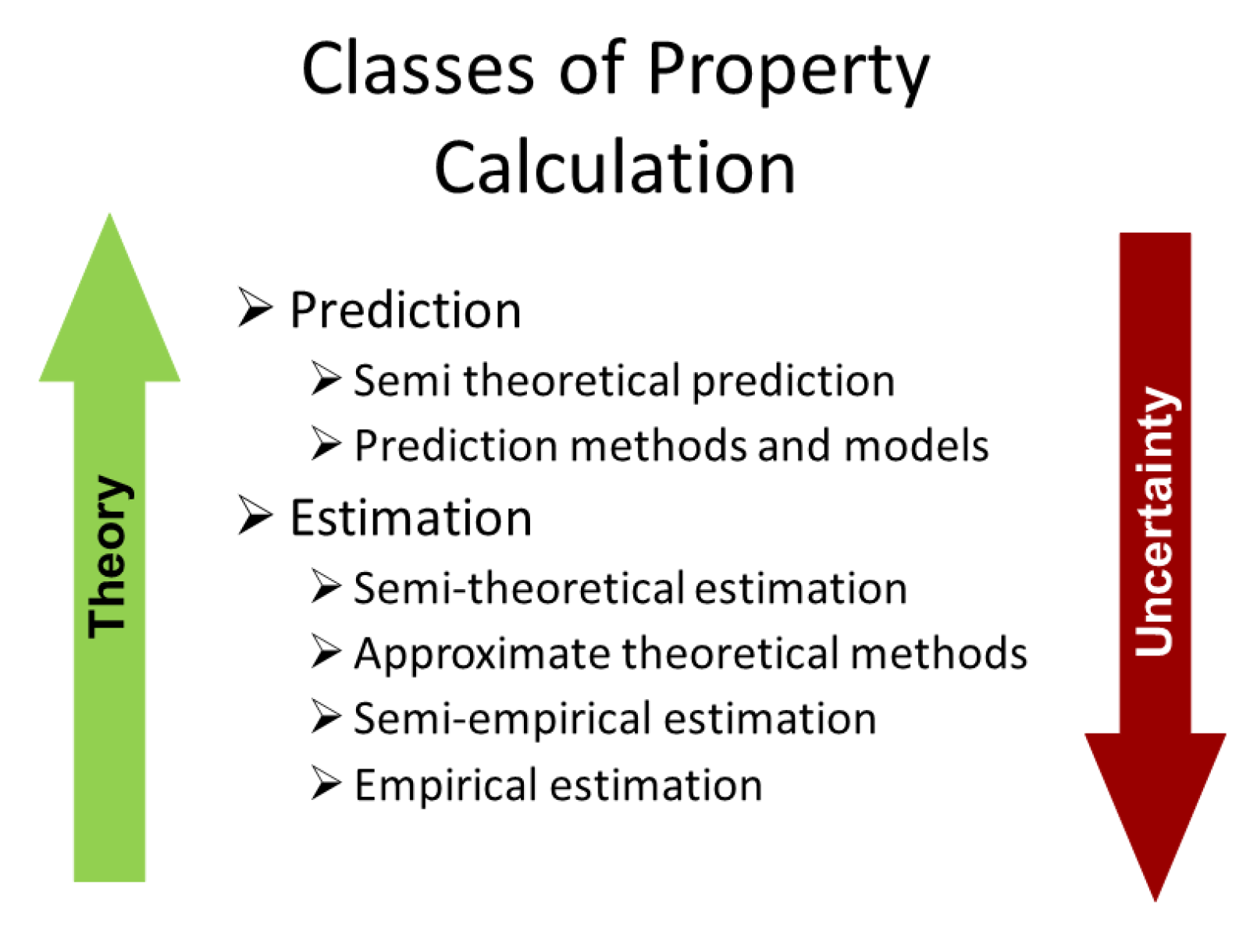
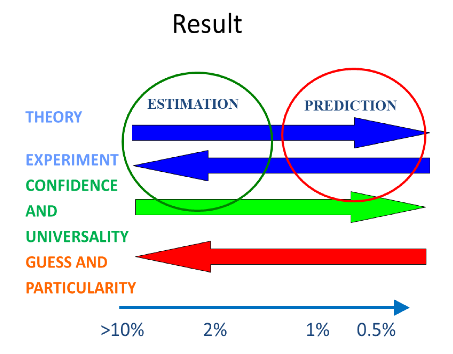
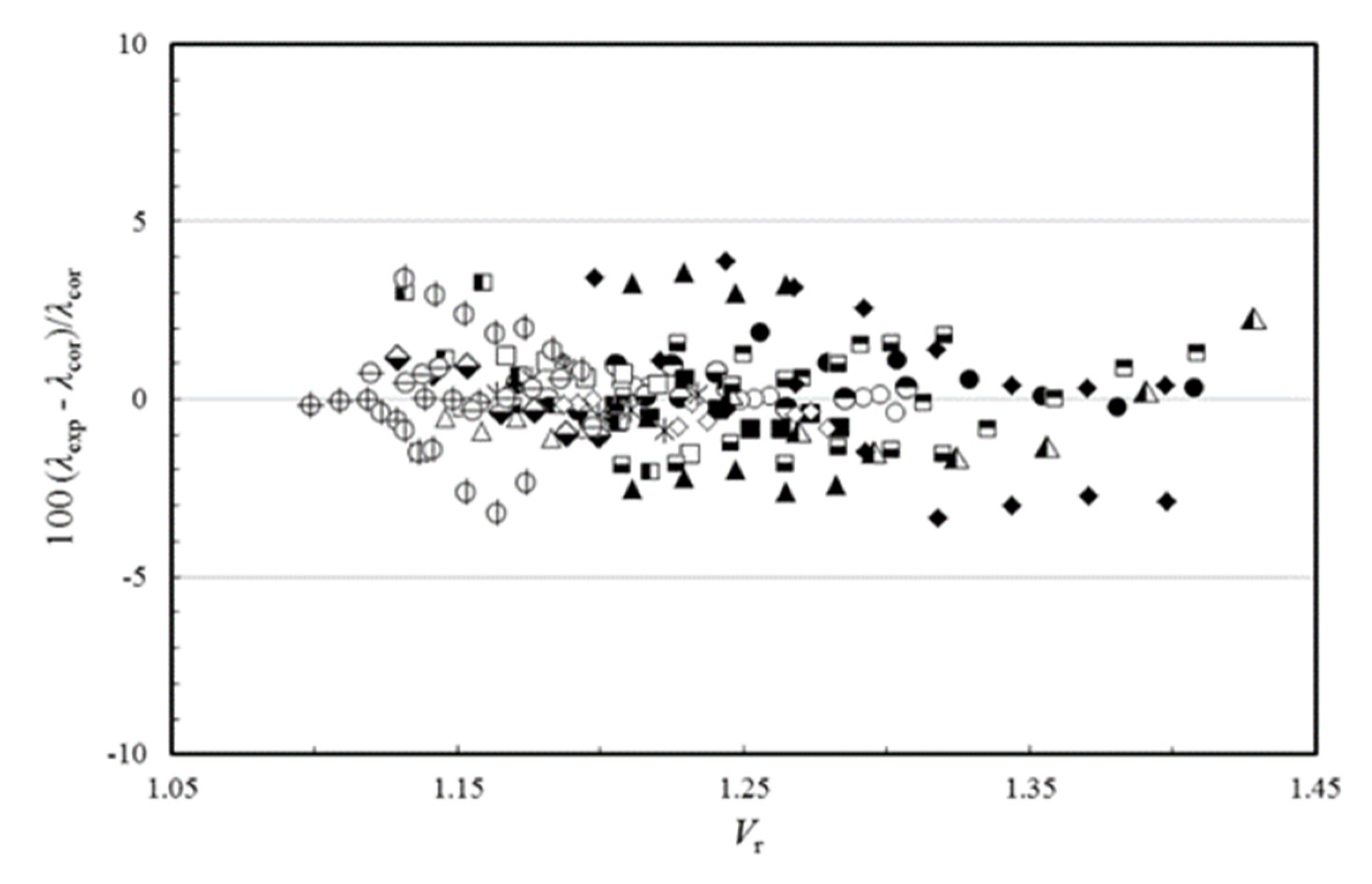
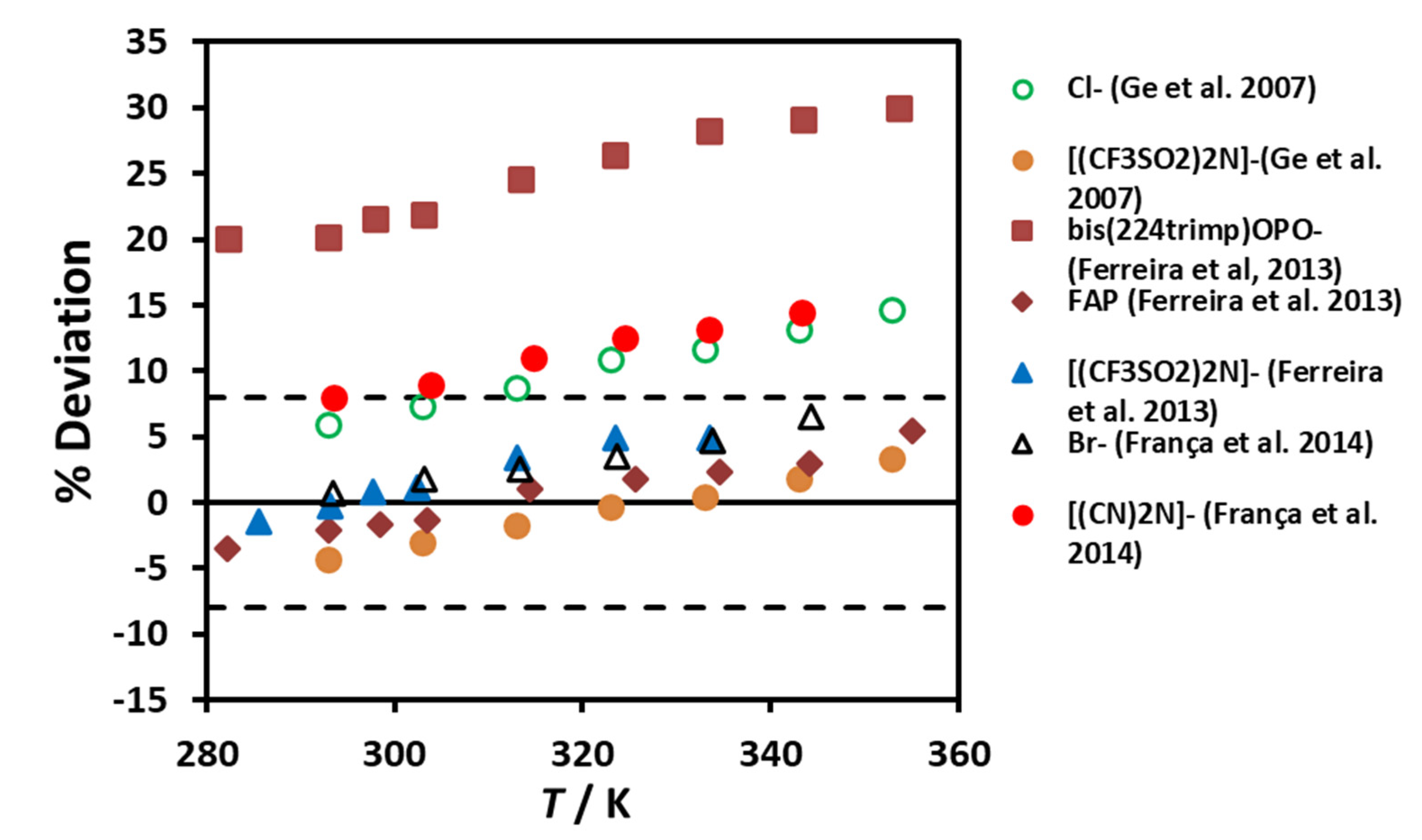
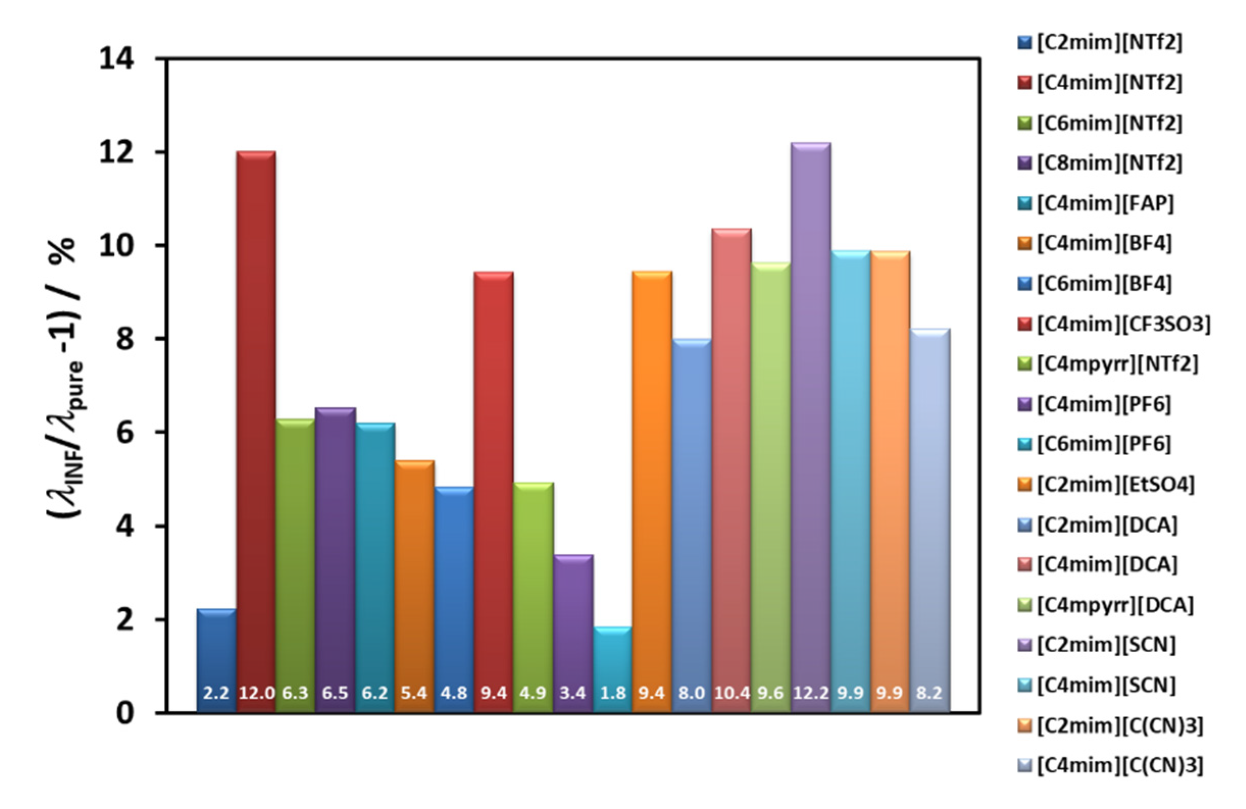
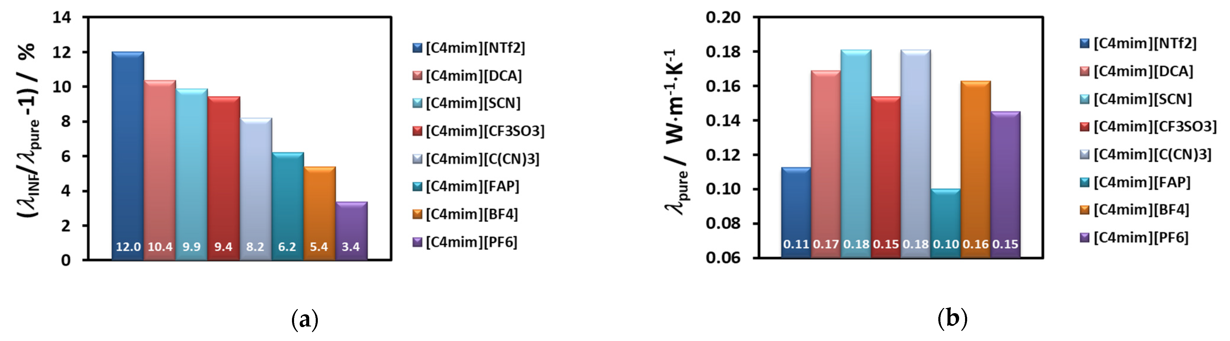
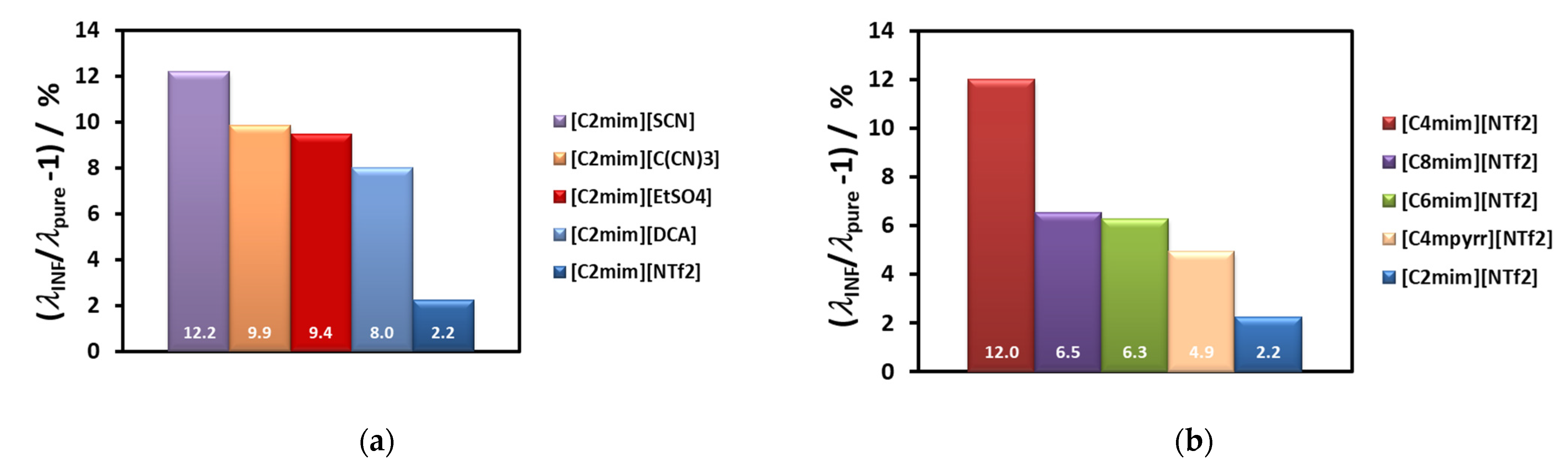
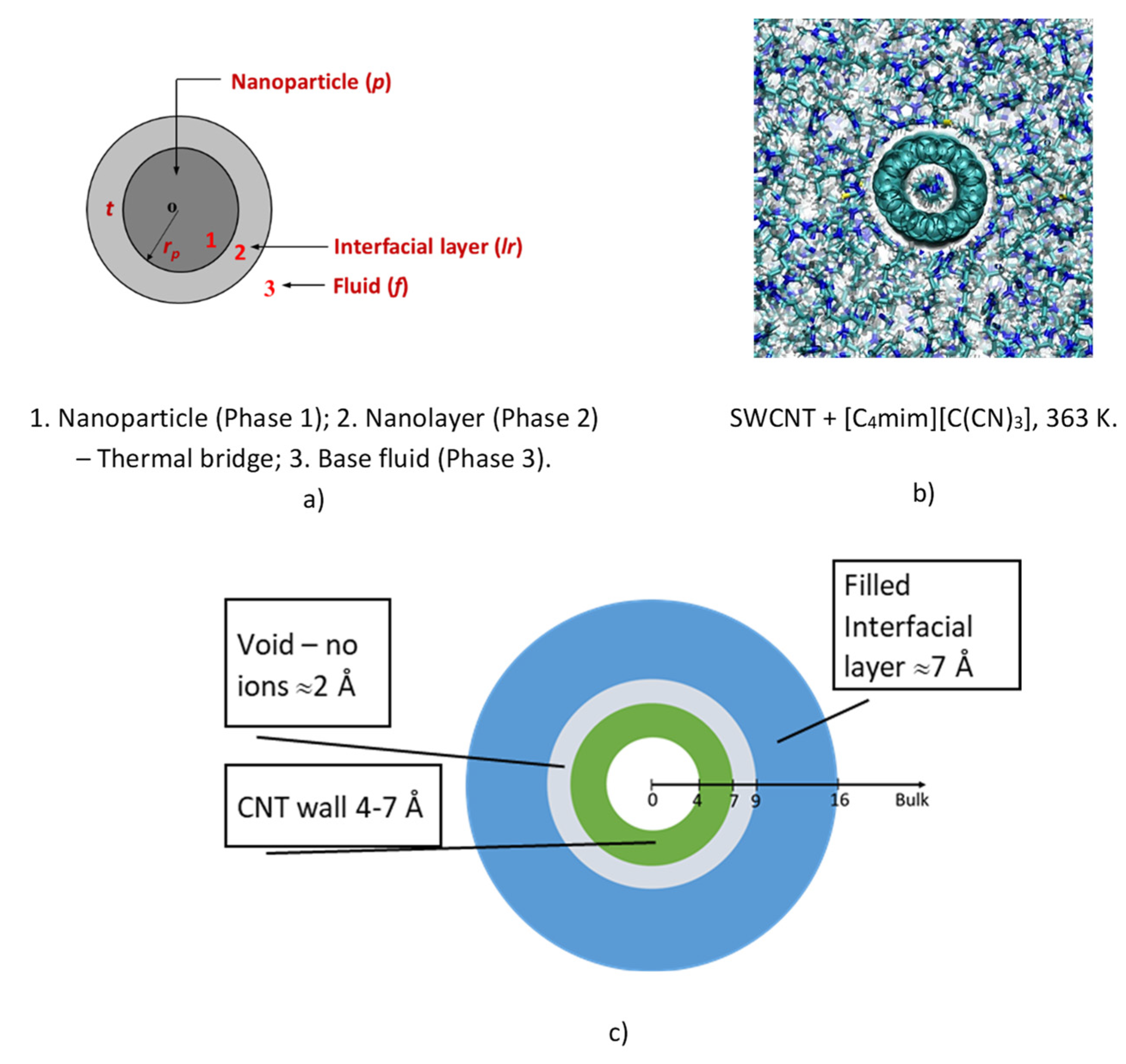
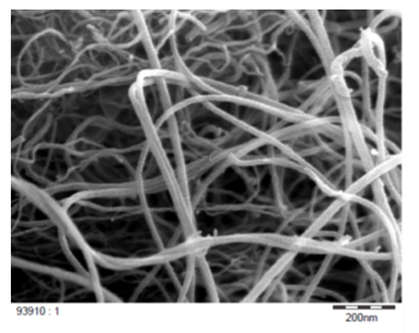
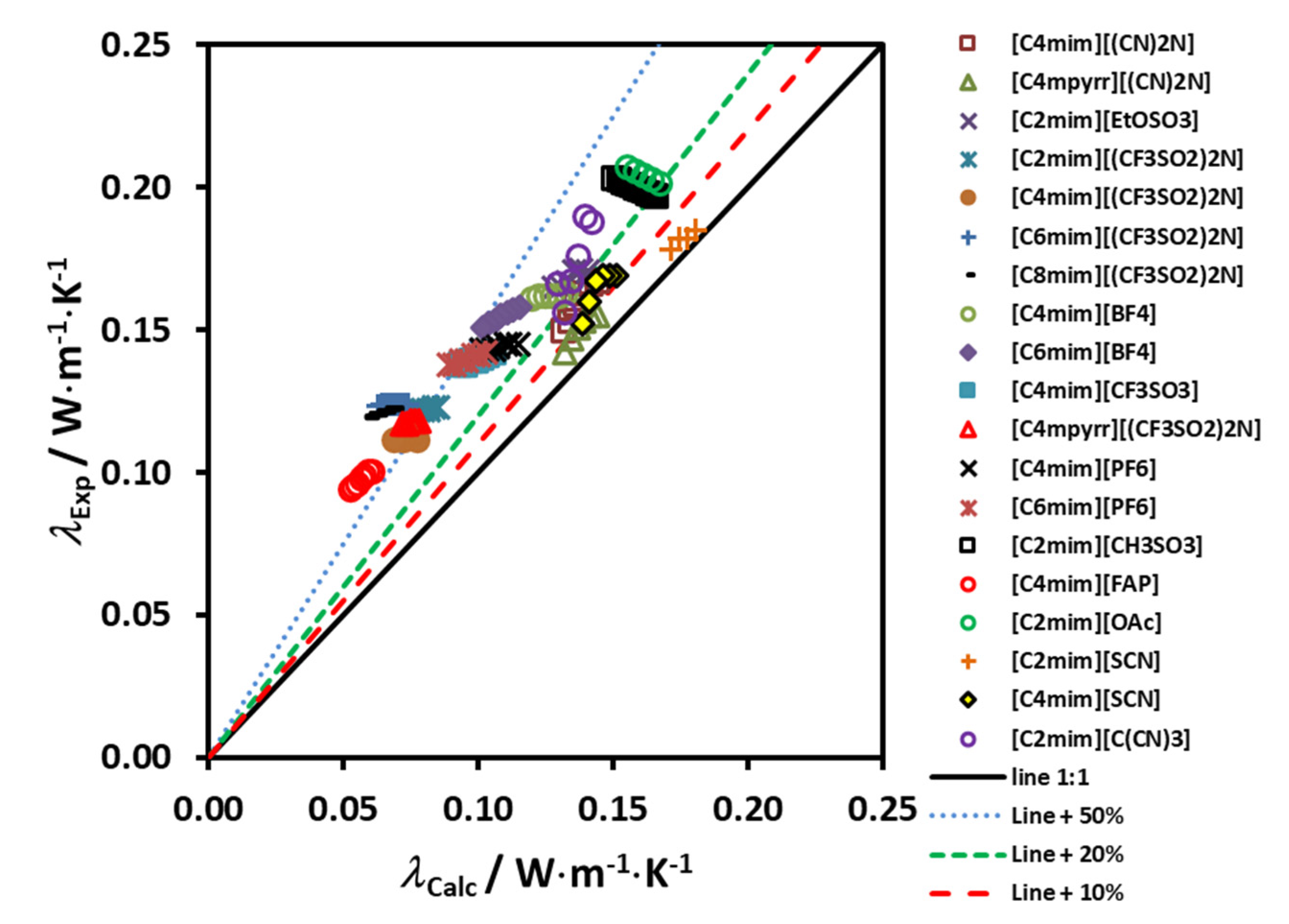
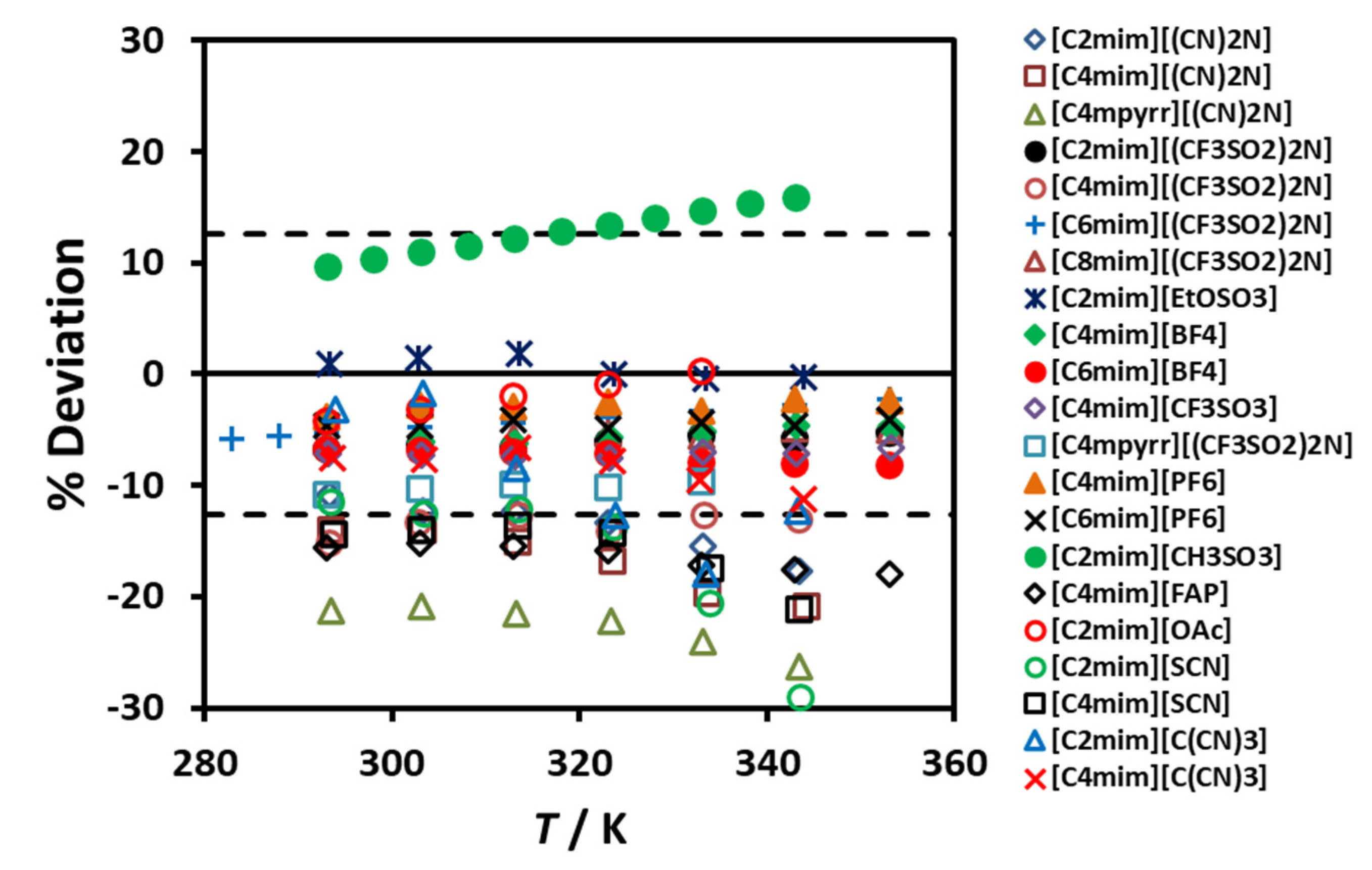
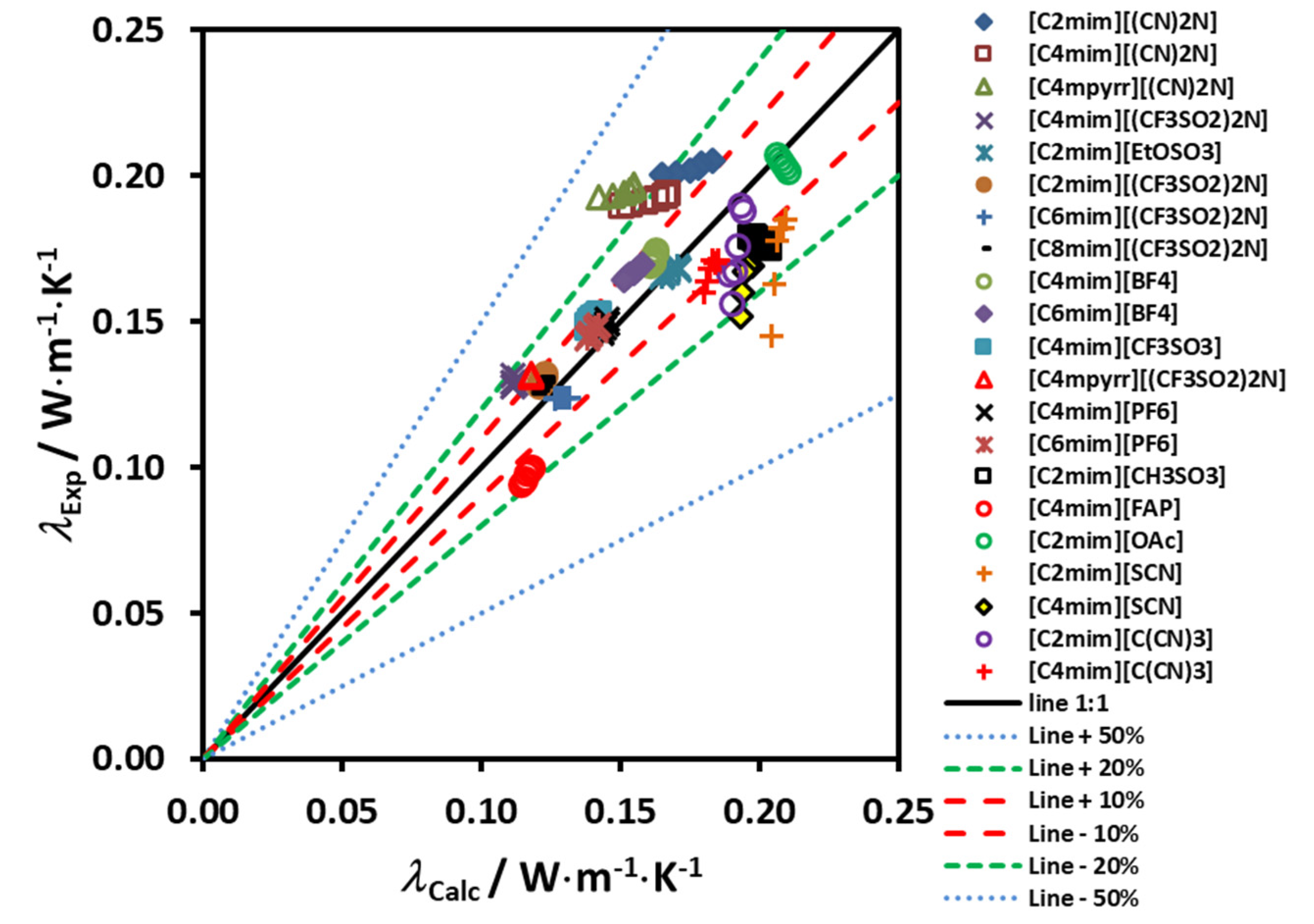
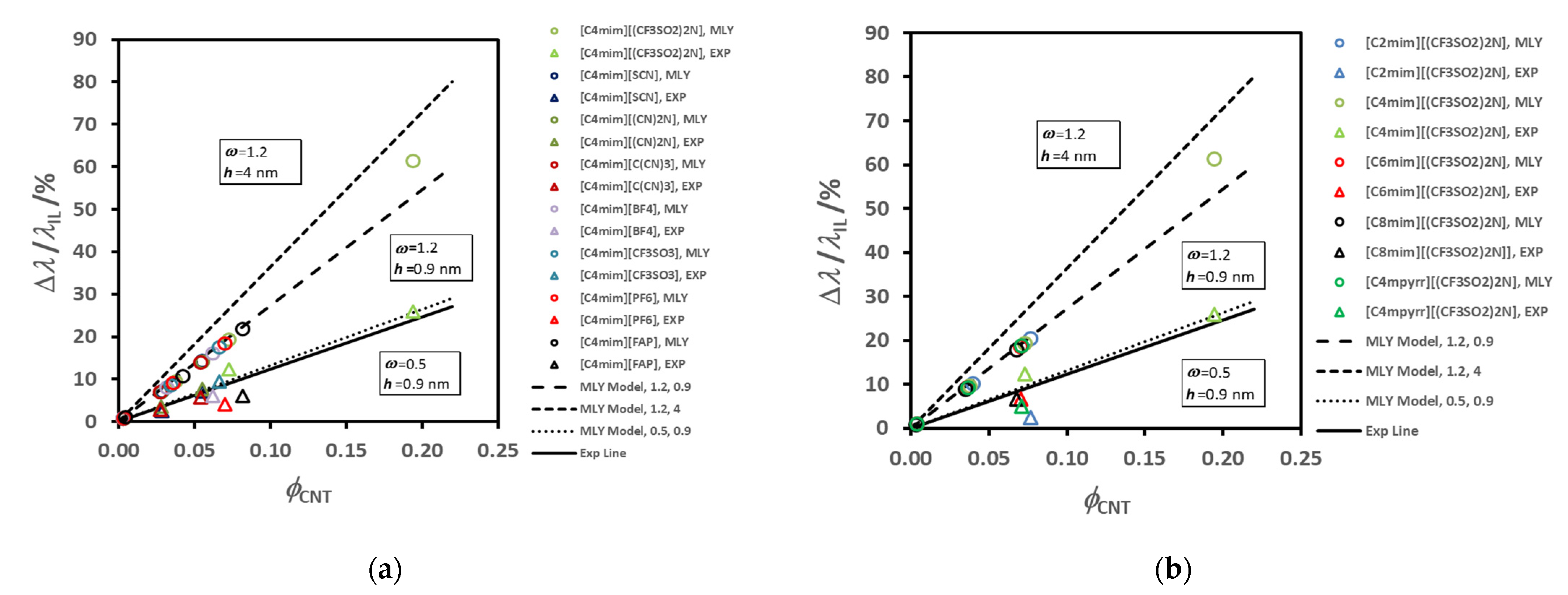
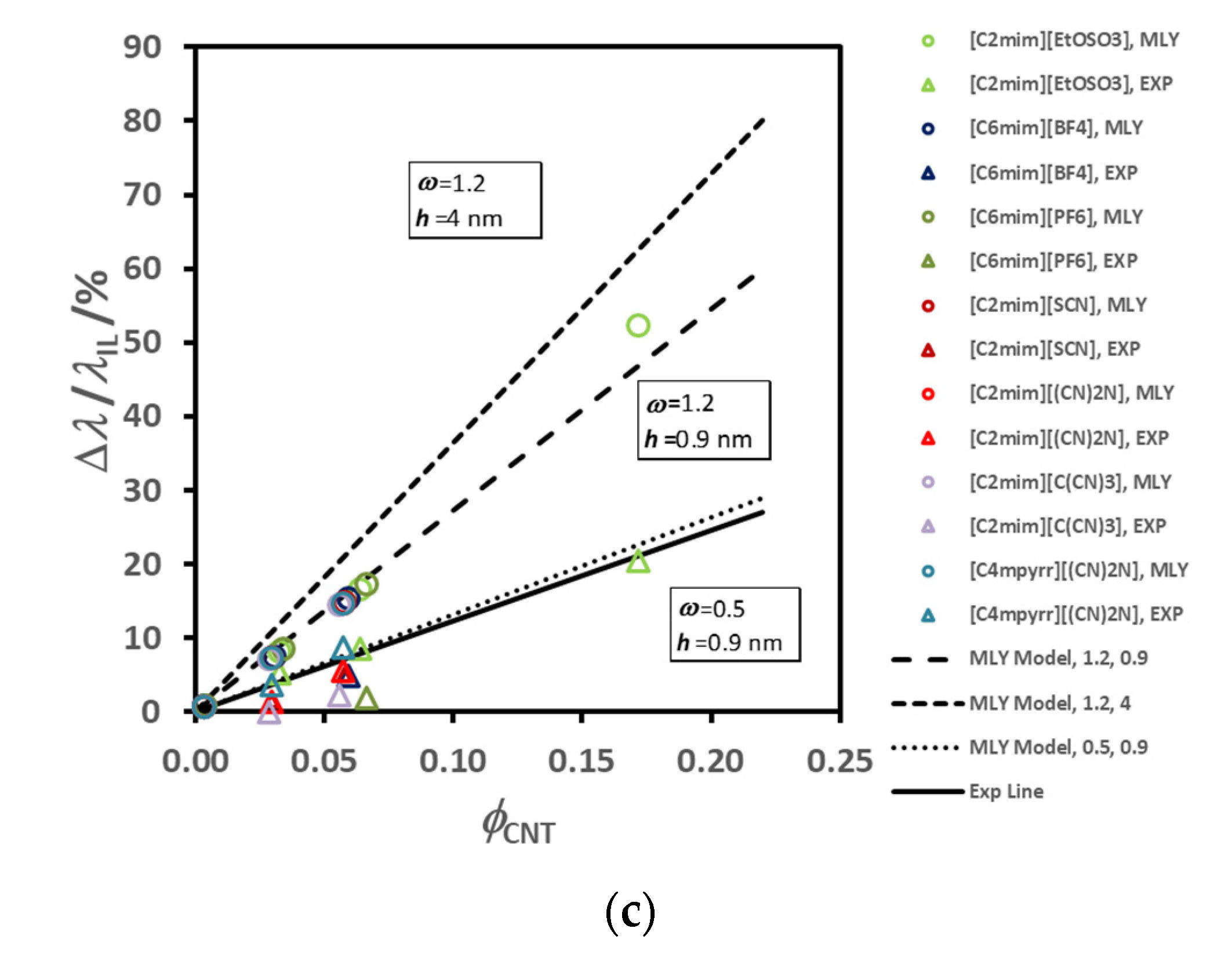
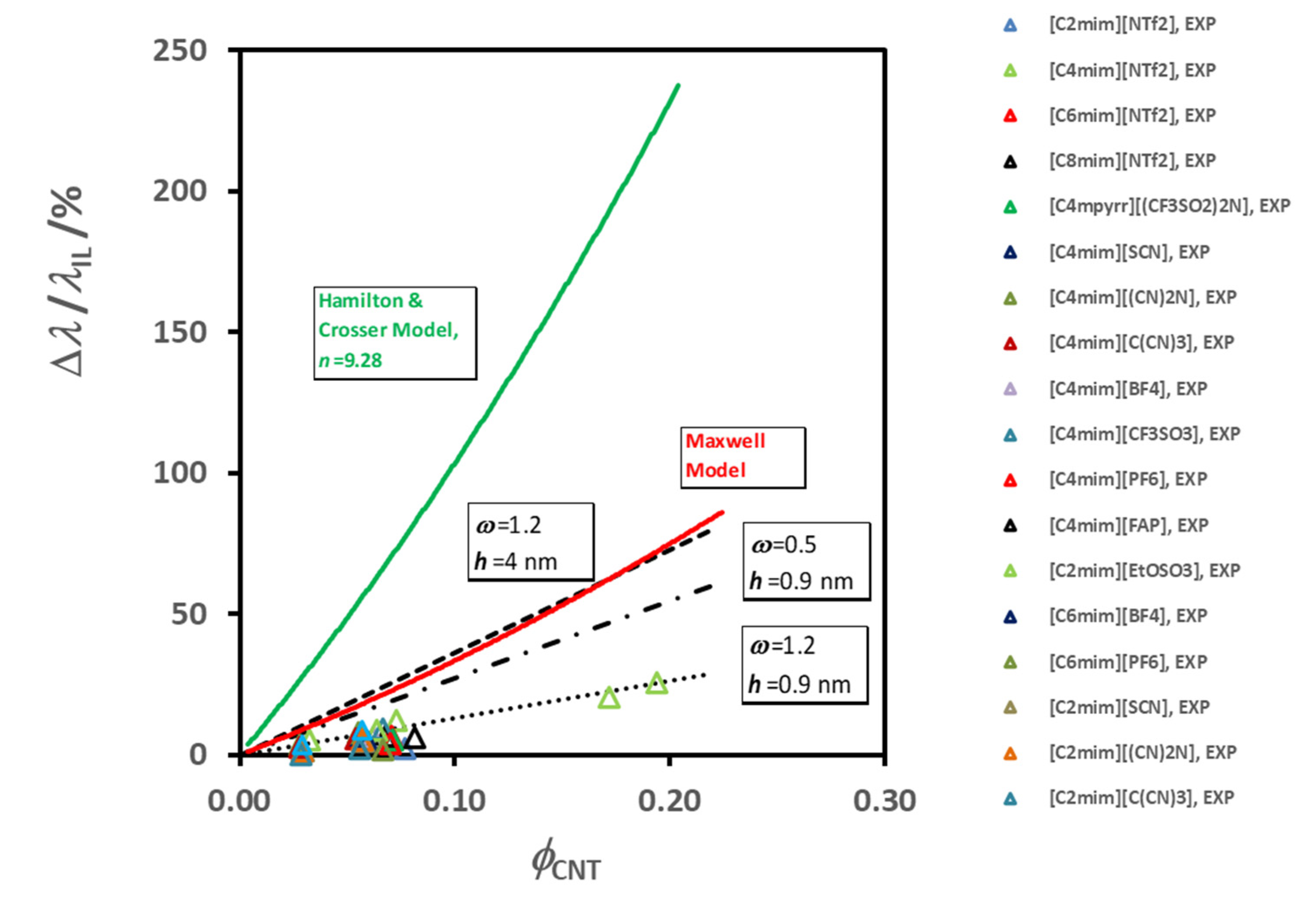
Table 1.
Current Ionic Liquids Moieties (Short List).
| Cations | Name | Anions | Name |
|---|---|---|---|
| [C4mim], [Bmim] | 1-butyl-3-methylimidazolium | [OCH3CO], [OAc] | acetate |
| [C4mpy], [Bmpy] | n-butyl-4-methylpyridinium | [B(CN)4] | tetracyanoborate |
| [C4mpyr], [Bmpyrr] | 1-butyl-1-methyl-pyrrolidinium | [BF4] | tetrafluoroborate |
| [Choline], [Cho] | 2-hydroxy-N,N,N-trimethylethan-1-ammonium | [Br] | bromide |
| [DMEA] | N,N-dimethylethanolammonium | [Cl] | chloride |
| [C2mim], [Emim] | 1-ethyl-3-methylimidazolium | [C4C4PO2], [DBP] | dibutylphosphate |
| [C2C2im], [Eeim] | 1-ethyl-3-ethylimidazolium | [N(CN)2], [DCA] | dicyanamide |
| [C2mpy], [Empy] | 1-ethyl-3-methylpyridinium | [C2C2PO2], [DEP] | diethylphosphate |
| [C2py], [Epy] | 1-ethylpyridinium | [C1C1PO2], [DMP] | dimethylphosphate |
| [C2OHmim] | 1-methyl-3-2-hydroxyethyl-imidazolium | [C2SO4], [EtSO4] | ethylsulfate |
| [C4C4im], [Bbim] | 1,3-dibutylimidazolium | [HSO4] | hydrogensulfate |
| [H2NC3H6mim] | 1-(3aminopropyl)-3-methylimidazolium | [I] | iodide |
| [HDEA] | diethanolammonium | [C1SO4], [MeSO4] | methylsulfate |
| [HEMA] | monoethanolammonium | [C1OSO2], [MeSO3] | methanesulfonate |
| [C6mim], [Hmim] | 1-hexyl-3-methylimidazolium | [NO3] | nitrate |
| [HTEA] | triethanolammonium | [CF3SO3], [OTf] | trifluoromethanesulfonate |
| [C1mim], [mmim] | 1,3-dimethylimidazolium | [PF6] | hexafluorophosphate |
| [C1mpy], [mmpy] | 1,3-dimethylpyridinium | [SCN] | thiocyanate |
| [OHemim] | 1-(2-hydroxyethyl)-3-methylimidazolium | [SO4] | sulfate |
| [C8mim], [Omim] | 1-octyl-3-methylimidazolium | [OCF3CO], [TFA] | trifluoroacetate |
| [P2444] | ethyl(tributyl)phosphonium | [(CF3SO2)2N], [NTf2], [Tf2N] | bis(trifluoromethylsulfonyl)imide |
| [P66614] | tetradecyl(trihexyl)phosphonium | [p-CH3C6H5SO3], [TOS] | Tosylate; p-toluenesulfonate |
| [N1114], [BA] | butylammonium | [(CN)3] | tricyanomethanide |
| [N1444], [TBA] | tributylammonium | [(C2F5)3PF3], [FAP] | tris(pentafluoroethyl)trifluorophosphate |
| [N1888], [OMA] | trioctylmethylammonium | [C1OHPO2] | methylphosphinate |
Publisher’s Note: MDPI stays neutral with regard to jurisdictional claims in published maps and institutional affiliations. |
© 2021 by the authors. Licensee MDPI, Basel, Switzerland. This article is an open access article distributed under the terms and conditions of the Creative Commons Attribution (CC BY) license (http://creativecommons.org/licenses/by/4.0/).
Share and Cite
MDPI and ACS Style
Paredes, X.; Lourenço, M.J.; Castro, C.N.d.; Wakeham, W. Thermal Conductivity of Ionic Liquids and IoNanofluids. Can Molecular Theory Help? Fluids 2021, 6, 116. https://0-doi-org.brum.beds.ac.uk/10.3390/fluids6030116
AMA Style
Paredes X, Lourenço MJ, Castro CNd, Wakeham W. Thermal Conductivity of Ionic Liquids and IoNanofluids. Can Molecular Theory Help? Fluids. 2021; 6(3):116. https://0-doi-org.brum.beds.ac.uk/10.3390/fluids6030116
Chicago/Turabian StyleParedes, Xavier, Maria José Lourenço, Carlos Nieto de Castro, and William Wakeham. 2021. "Thermal Conductivity of Ionic Liquids and IoNanofluids. Can Molecular Theory Help?" Fluids 6, no. 3: 116. https://0-doi-org.brum.beds.ac.uk/10.3390/fluids6030116