
Hydrodynamic Characterisation of a Garman-Type Hydrokinetic Turbine


1
PAI+ Group, Energetics & Mechanics Department, Faculty of Engineering, Universidad Autónoma de Occidente, Cali 760030, Colombia
2
Mathematics, Informatics & Engineering Department, University of Quebec at Rimouski, Rimouski, QC G5L 3A1, Canada
3
Computational Mechanics Research Group, Mechanical Engineering Department, Faculty of Engineering, Universidad de los Andes, Bogotá 111711, Colombia
*
Author to whom correspondence should be addressed.
Fluids 2021, 6(5), 186; https://0-doi-org.brum.beds.ac.uk/10.3390/fluids6050186
Submission received: 26 March 2021
/
Revised: 6 May 2021
/
Accepted: 6 May 2021
/
Published: 14 May 2021
(This article belongs to the Special Issue Modelling and Simulation of Turbulent Flows)
Abstract
:This paper presents a numerical study of the effects of the inclination angle of the turbine rotation axis with respect to the main flow direction on the performance of a prototype hydrokinetic turbine of the Garman type. In particular, the torque and force coefficients are evaluated as a function of the turbine angular velocity and axis operation angle regarding the mainstream direction. To accomplish this purpose, transient simulations are performed using a commercial solver (ANSYS-Fluent v. 19). Turbulent features of the flow are modelled by the shear stress transport (SST) transitional turbulence model, and results are compared with those obtained with its basic version (i.e., nontransitional), hereafter called standard. The behaviour of the power and force coefficients for the various considered tip speed ratios are presented. Pressure and skin friction coefficients on the blades are analysed at each computed turbine angular speed by means of contour plots and two-dimensional profiles. Moreover, the pressure and viscous contributions to the torque and forces experienced by the hydrokinetic turbine are examined in detail. It is demonstrated that the reason behind the higher power coefficient predictions of the transitional turbulence model, close to 6% at maximum efficiency, regarding its standard counterpart, is the smaller computed viscous torque contribution in the former. As a result, the power coefficient of the inclined turbine is around 35% versus the 45% obtained for the turbine with its rotation axis parallel to flow direction.
1. Introduction
The fast development of renewable energy technology is responsible for the increase of the renewable sources in the world energy production (2537 GW in 2019, with an increase of 7% regarding 2018, constituting nowadays more than one-third of the global power production). By far, the highest contribution comes from hydropower which accounts for 48% of total installed capacity or renewables with 1300 GW [1].
Following [2], water transport systems, based on their kinetic energy, are an interesting renewable energy resource, in addition to conventional hydropower. This kind of energy can be obtained by employing previously developed infrastructures avoiding water impoundment; therefore, expenses connected with civil works and the building of specific generation centrals can be reduced. On the other hand, impact in the environment is minimal since the visual impact is scarce, and there are no emissions or noise. Moreover, the development of novel technologies has made possible the efficient exploitation of the resource. Such benefits of water streams have attracted attention in recent years, both as an energy source and for providing electricity to remote areas far from the electrical grid [3,4,5].
For satisfying electricity needs of communities or services located close to a water stream, a reliable and inexpensive option is the use of current energy conversion (CEC) systems which consist of a hydrokinetic turbine (HK) immersed in the flowing water [6]; this device is able to generate energy without the need of potential energy head. For this reason, they are called zero-head CEC. However, as pointed out and discussed at length by Kirke [4], this assertion is a “myth” as, for instance, CECs cause a slight increase in the level of water upstream (slowing down the flow) when they are used in confined environments, and hence, they do not operate exactly with zero-head. HK turbines can be deployed in any stream with an established, predictable flow, provided that some conditions of a minimum depth, volumetric flow, and velocity are fulfilled. Such locations include natural rivers, weirs, derivations, irrigation channels, low-height dams, etc. [7]. Since hydrokinetic devices harness energy from the water motion (i.e., kinetic energy), their design tends to be simple and often is inspired by that of wind turbines. Moreover, HK turbines have minimal impact on the environment, with low installation and maintenance costs. For these reasons, they are an attractive option to be used in rural, isolated areas [8].
There are two major types of CEC devices, according to the orientation of the rotational axis regarding the flow stream. The axial machines have is rotor normal to the current, while the crossflow turbines operate with their rotation axis oriented 90° with respect to the flow direction in a horizontal or vertical arrangement. Although the former are more efficient in energy conversion, the latter are independent of stream orientation, which makes them attractive for being employed as tidal CEC. A classification of hydrokinetic CECs can be found in [2].
In the last years, some extensive reviews about the technology, challenges, and simulation of HKs have been published, e.g., [2,9,10]. Therefore, we refer the reader to these papers for a thorough panorama of the recent context and development of hydrokinetic turbines.
A remarkable fact to be mentioned is that the development of HKs has been performed mainly empirically and less frequently by computational fluid dynamics (CFD), dealing with issues such as maintenance, anchoring strategies, debris safeguard, etc. [11,12]. This fact is because of the complexity of the flow around hydrokinetic turbines which prevents a purely theoretical approach. In order to improve their performance, a profound comprehension of the relevant hydrodynamic phenomena is needed. A tool that aims to this objective is computational fluid dynamics (CFD), which has been applied during the last years to investigate the flow development around HKs; a recent review on this topic can be found in [10]. In CFD, the fluid mechanics’ conservation equations (i.e., mass, momentum, and energy) are solved employing numerical methods, which enable CFD to deal with general, often complicated, geometries in a comprehensive manner. Nowadays, CFD has been adopted in nearly all the fields of engineering as a reliable tool for the design, improvement, and troubleshooting of all kinds of fluid systems (e.g., [13,14,15,16,17,18,19,20,21,22,23,24]). For this reason, it has been the approximation employed in the current work.
A context for the present study is provided in the following. Colombia is a country that covers a surface of 1.14 million km2 where approximately 80% of the population is concentrated in cities; this fact has as consequence the existence of vast rural areas without access to the national electrical grid, around 52% of the territory, known as the nonconnected zones (NCZs). On the other hand, these areas have available abundant water resources flowing in a number of rivers and streams. Therefore, HK technology is an attractive alternative for the production of electricity in the NCZ since they are easy to install and have low maintenance costs that can be afforded by local communities. In particular, the Orinoco and Amazonas basins as well as the Andean basin in Colombia, present a good number of wide and deep rivers, even with high flow, in which hydrokinetic turbines could be deployed.
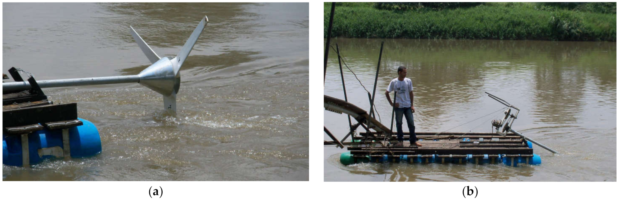
Historically, the Garman turbine was one of the first developed hydrokinetic turbines [9]. It is an axial turbine whose design resembles that of a wind turbine. The company Thropton Energy (http://www.throptonenergy.co.uk/, accessed on 5 May 2021) developed during the years several machines with variable rotor diameter between 1.8 and 4 m which operate with the rotation axis inclined a certain angle regarding the flow direction. They deployed this kind of turbine in Peru and in the Nile River (north of Sudan) for pumping water and irrigation applications where more than 15,000 h of operation were reported [12]. As a result of collaboration between Thropton Energy and the local engineering firm Aprotec, an empirically adapted Garman turbine was developed in Cali (Colombia), redesigning the hub and the rotor. This turbine was named Aquavatio, and it was in operation in the Cauca River during several campaigns during the years 2010–2011 in which its feasibility was assessed. Figure 1 shows two photographs of the prototype which, during its operation period, provided a power of around 450 W on average. However, because of its on-site operation, this turbine was never properly characterised from an experimental point of view.
Given that reliable experimental data on Aquavatio do not exist, this paper deals with the detailed CFD simulation of the Aquavatio HK aimed at two objectives: building the efficiency curve and characterizing its hydrodynamic behaviour depending on the inclination angle of the turbine rotation axis regarding the flow direction (see Figure 2 below) and rotor angular speed . The sensitivity of the global parameters (power coefficient and thrust on the rotor) versus the modeling of the boundary layer development along the blades, either fully turbulent or including the transition from laminar to turbulent, is also studied. Moreover, a detailed analysis of pressure and skin friction coefficients obtained by both modeling alternatives is presented. Finally, the dependence of the intermittency contours with the turbine axis orientation angle is illustrated for three turbine rotational velocities.
2. Geometrical Model and Numerical Setup
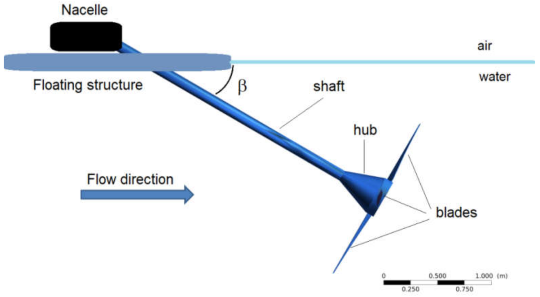
As commented in the introduction, the considered HK turbine of Garman type is a prototype named Aquavatio, which was constructed adapting the design of a Garman turbine with the rotor of a previous wind turbine [25]. Such empirically designed machine was in operation some years ago on the Cauca River, in the southwest of Colombia. However, although its feasibility was demonstrated in situ, no reliable experimental measurements could be carried out. Figure 2 shows schematically the real operation of this turbine: it works with the shaft inclined at an angle with respect to the stream direction where the flow approaches the rotor downstream the floating structure. The generator and transmission system are located on the barge in the nacelle.
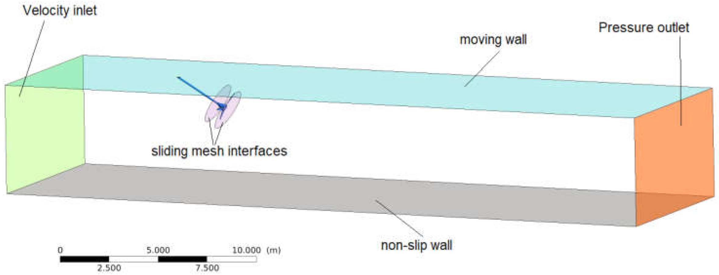
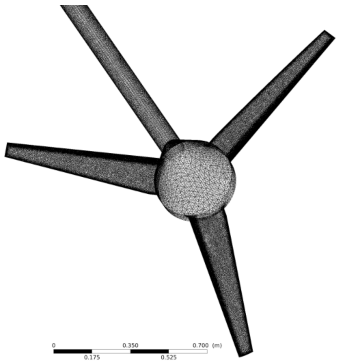
The employed computational domain is shown in Figure 3, whereas Figure 4 presents a detail of the surface mesh on the rotor and shaft.
The computational domain consists of a rectangular box of length 20, width 6, and total height 4, where represents the turbine diameter. Inside of it, a disc-like subdomain containing the rotor (hub and blades), is located, whose dimensions are as follows: diameter 1.2 and thickness 0.5. It constitutes the rotating subdomain, while the stationary subzone comprises the rest of the numerical domain. Both subdomains are connected by interfaces of the sliding mesh type in order to reproduce the physical rotation of the blades. In Figure 3, flow progresses from left to right; the green boundary is defined as a velocity inlet, where a fixed water velocity is imposed normal to the boundary; the orange surface is specified as a pressure outlet with 0 Pa; the upper (cyan) boundary, being the free surface, was established as a moving wall with the same velocity as the fluid at the inlet; the rest of borders (i.e., bottom and side boundaries) are standard fixed walls where the nonslip condition is enforced. Of course, at the walls of the turbine, also the nonslip requirement is imposed. The tip speed ratio (TSR), , was computed from specified values for the rotor angular velocity, , as follows:
In Equation (1), denotes the turbine radius, and the water incoming velocity.
The spatial discretization of the computational domain is performed by a nonstructured grid based on tetras constructed with the commercial software ANSYS ICEM-CFD v19. As it can be seen in Figure 4, the surface mesh on the rotor is quite uniform and denser near the blades’ tip and trailing edge. Adequate description of the boundary layer around the blades is achieved by means of at least 20 prisms layers with a growth rate of 1.1, which guarantees values of around 1 in such surfaces (width of the first prisms layer 0.013 mm). Additionally, the element aspect ratio of the outer unstructured grid was kept similar to that of the prisms to establish an appropriate connection between the grids in both regions. Finally, the mesh density was higher in the turbine wake due to the complex flow features in that zone.
The shear stress transport model (SST) of Menter [26,27,28] was employed to describe the flow turbulence using both, standard and transitional versions, available on the commercial simulation software ANSYS-Fluent v. 19. Both approaches have been previously employed to simulate the flow around hydrokinetic turbines, horizontal, and vertical axis [22,24,29,30,31,32] providing results close to the experiments. The transitional version of the model (SST–Tr) implements a formulation that includes a model for the transition from laminar to the turbulent boundary layer, while the standard (SST–St) assumes a fully turbulent boundary layer. The reason for using a transition turbulence model is that physically several phenomena are actually happening in the boundary layer around the rotating blades, such as laminar boundary layer, transition to turbulence, laminar separation, flow reattachment, and turbulent separation. Typically, a fully turbulent boundary layer model cannot predict or capture these phenomena, even though the production of turbulent kinetic energy can be controlled with a damping function. In the case of the SST transition model, two extra equations control the laminar–turbulence transition: one for the intermittency (fraction of time that flow is turbulent in the boundary layer) and the other for the transition momentum thickness Reynolds number [28]. Such laminar-to-turbulent flow transition within the boundary layer affects the wall shear stress distribution on the blades and has a moderate effect on turbine performance, as it will be shown below. As stated in the introduction, the present contribution analyses the results of pressure and skin friction coefficients obtained by both modelling alternatives.
From a numerical point of view, second-order schemes are employed for the spatial discretization of all the relevant transport equations; moreover, time is discretized by an implicit second-order scheme. The time step was chosen as that corresponding to 0.8 degrees of blade rotation; therefore, it varies with the considered TSR. The transient semi-implicit method for pressure linked equation (Transient SIMPLE) algorithm is used for the coupling of pressure and momentum equations. At each time step, convergence is attained when residuals reached 10−5. The transient simulation is run for several turns up to the moment in which the total torque difference between consecutive revolutions is lower than 0.5%.
3. Verification and Validation of the Simulation Strategy
In this study, two HK turbine configurations are simulated. The first one considers the rotor orthogonal to the flow direction, hence labelled as PP, and the second assumes an inclination angle regarding the free surface , labelled as TI. A grid independence study was performed for the parallel configuration following the standard approach. Three grids with different numbers of elements are simulated: a coarse mesh (5 million), a medium mesh (8 million), and a refined mesh (10.5 million). The study is carried out for a rotational velocity of rpm, where the turbine presents its maximum efficiency, using the SST–Tr turbulence model. The obtained torque coefficients are coarse 0.0784, medium 0.0819, and refined 0.0825. Since the discrepancy between the fine and intermediate grids is lower than 1%, the last one is employed in the simulations as a compromise between accuracy and computational cost. For the inclined rotor case, also a mesh with around 8 million elements was considered appropriate.
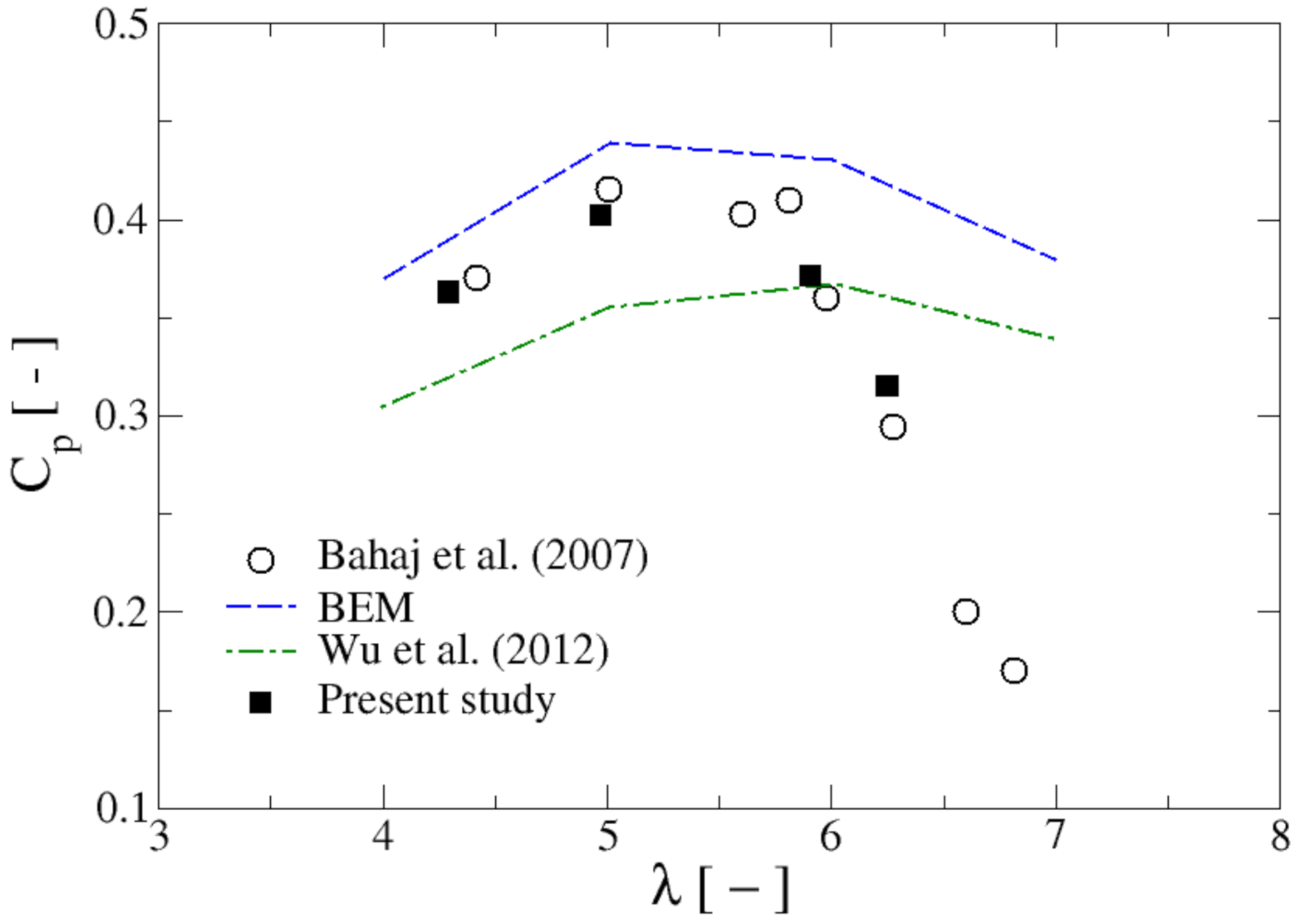
As commented previously, the Aquavatio turbine was empirically built and always operated on-site, and therefore, an accurate experimental characterisation was never performed. As a validation alternative, another well-known horizontal axis HK turbine has been chosen. This is the Bahaj et al. turbine [33] which has been frequently employed to validate numerical methods and computational methodologies [33,34]. This turbine has three blades with the rotor perpendicularly oriented regarding the flow.
The employed numerical setup in the simulation was similar to that employed for the inclined turbine. The rotor diameter of the hydrokinetic turbine [33] was = 0.8 m with blades based on the profile shape of a NACA 63-8XX (XX are two digits indicating the profile thickness–chord ratio, which ranges from 12 to 24 in this case); the information about the chord, thickness, and pitch was taken from [33]. The computational domain consisted of two subdomains: a rotating part and a steady one. The rotating domain had the shape of a cylinder and included the turbine rotor. The spatial discretization was carried out by an unstructured grid based on tetras and consisted of around 8.5 million elements. Approximately 80% of the cells in the computational domain were located in the rotating cylinder; mesh refinement is necessary along the rotor blades in order to fulfill the near-wall treatment. Then, 15 layers with an inflation of 1.15 were set in ANSYS Meshing 19.0 to capture the boundary layer development around the blades and hub walls. The static domain was prismatic with an inner hole to fit the rotating domain. Different mesh sizes were employed in order to improve the resolution of the domain interfaces and the downstream wake. Governing equations were discretized using second-order schemes in space and time, where the transient flow was computed by the sliding mesh technique.
Figure 5 shows the obtained computational results for the power coefficient in the present study. Apart from the experiments [33], some other computational results are shown in that figure: the BEM results of [33] and the CFD predictions of [34], based on the standard k-ε turbulence model. As it can be readily seen the presented results, values based on the transitional SST turbulence model are closer to the experimental data than the other two, which demonstrates the ability of CFD simulations, combined with a proper turbulence model, for being used in the design and evaluation of hydrokinetic turbines.
In Figure 5 the power coefficient is defined as follows:
In Equation (2) , denotes the torque that the water transfers to the rotor and the fluid density. In this paper, the terms rotational speed and tip speed ratio are used interchangeably for referring to the considered turbine operational points. Other relevant coefficients are the torque coefficient and the normal force or thrust coefficient (component perpendicular to the rotor); they are expressed as follows:
where is the normal component of the hydrodynamic force acting on the rotor, i.e., the thrust.
4. Results for Integral Parameters
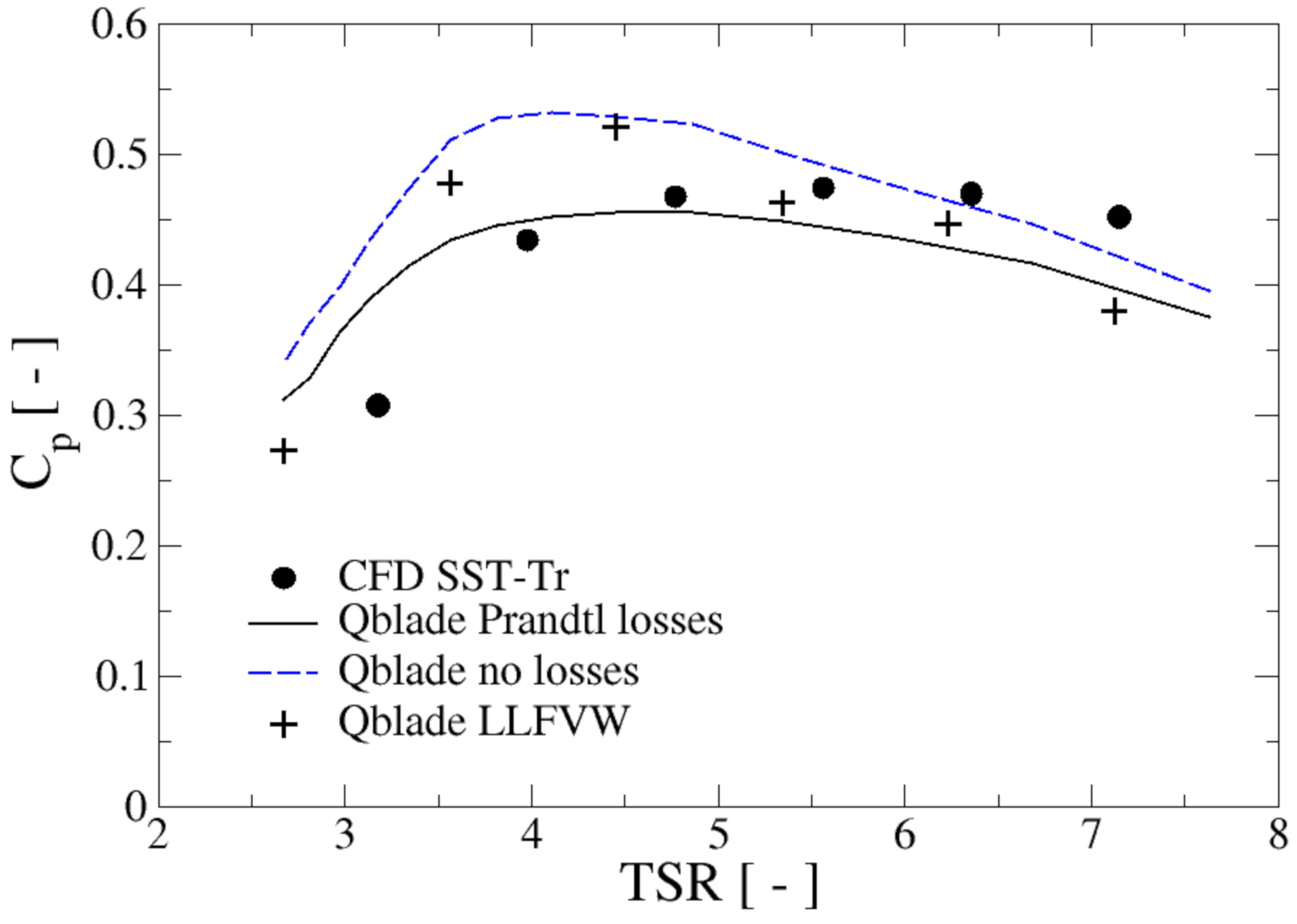
Simulations are carried out for the two rotor configurations, perpendicular to the flow direction (PP configuration) and tilted an angle with respect to it (TI configuration); see Figure 2. First, the power coefficient results of the present CFD simulations for the PP rotor are compared with those obtained by other simplified methods based on potential flow approximations. The first one is the blade element momentum (BEM) approach as it is implemented in the software package Qblade, and the second method is the lifting line free vortex wake (LLFVW), also included in the same package. Qblade is a general-purpose open source software for the aerodynamic design and analysis of wind turbines (horizontal and vertical axis) which is coupled with additional aeroelastic and structural modules [35]. Nevertheless, the fluid properties can be modified; therefore, it can be applied to HK turbines. In the BEM method, in addition to the ideal case, another simulation including the tip and root Prandtl losses has been performed. The BEM approach has been very much used in the analysis and design of HK turbines (e.g., [32,36,37]). On the other hand, the LLFVW approach is one of the most sophisticated simplified vortex models and allows for the free development of the wake as the flow progresses through the turbine [38].
The computed curves with the considered numerical approaches are presented in Figure 6. As it can be readily seen, all the curves are qualitatively similar in shape, although the CFD computations (performed with the SST–Tr turbulence model) show a flatter profile than the other approaches for TSRs between 4 and 7. In particular, all the Qblade results provide lower values than CFD for the highest range of and higher than those of CFD for the lowest values of the tip speed ratio. As a consequence, the CFD computations suggest an optimum TSR higher than the other approaches. Expectedly, the BEM simulation curve including the Prandtl losses is below that of the corresponding ideal case, while the LLFVW results mainly lie between both curves. All numerical approaches predict a sudden drop of power coefficient for tip speed ratios lower than around four, attributed to the dynamic stall experienced by the blades. Overall, the agreement among the various approaches is remarkable; however, the advantage of the CFD over potential methods is its ability to provide a large amount of data on the flow field around the HK turbine and the distribution of forces and torques acting on the rotor along with its time evolution.
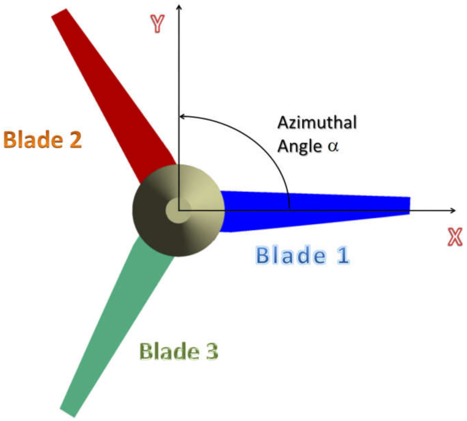
In the following, a detailed study of the variation of the hydrodynamic coefficients with the turbine rotational speed (i.e, tip speed ratio) is performed. For that, five rotor angular velocities,, have been selected, which allows the construction of the efficiency curve . As a first stage, the behaviour of the power and force coefficients of one blade along a revolution is analysed as a function of the tip speed ratio for the PP and TI arrangements. The employed turbulence model in this study is the SST Transition [28].
Figure 7 shows the employed coordinate system and illustrates the azimuthal angle which increases counterclockwise from 0° to 360°. It should be remarked that, in the PP configuration, the flow field seen by the blade along its whole revolution is basically identical; in other words, from the point of view of the flow field, all blade azimuthal positions are essentially equivalent. This fact implies that in this case both coefficients (thrust and power) are roughly constant with , showing only a small variation. This is not the case for the inclined turbine, in which the flow conditions experienced by the blade clearly change along a turn. Therefore, in this case, a fairly periodic behaviour of the coefficients could be expected.
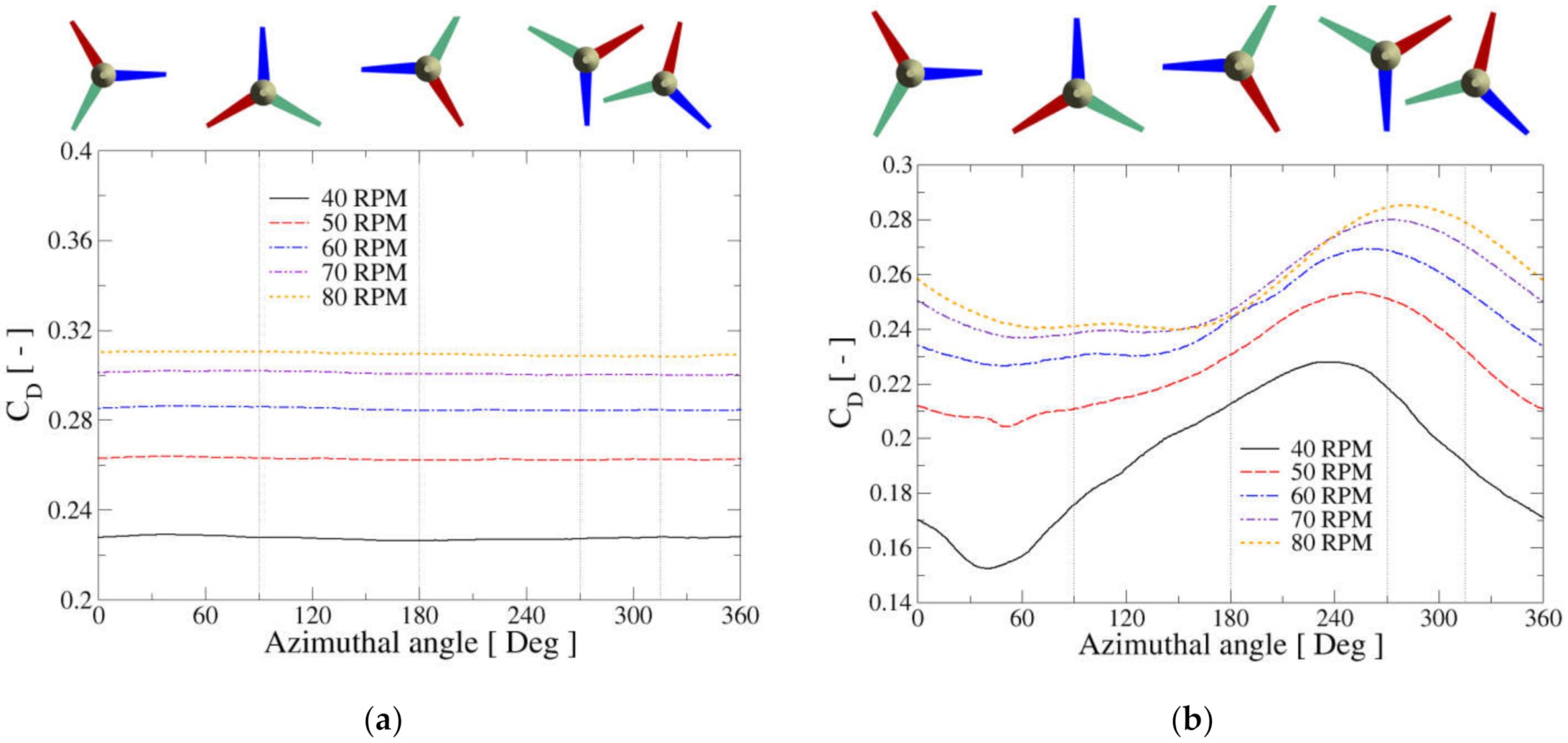
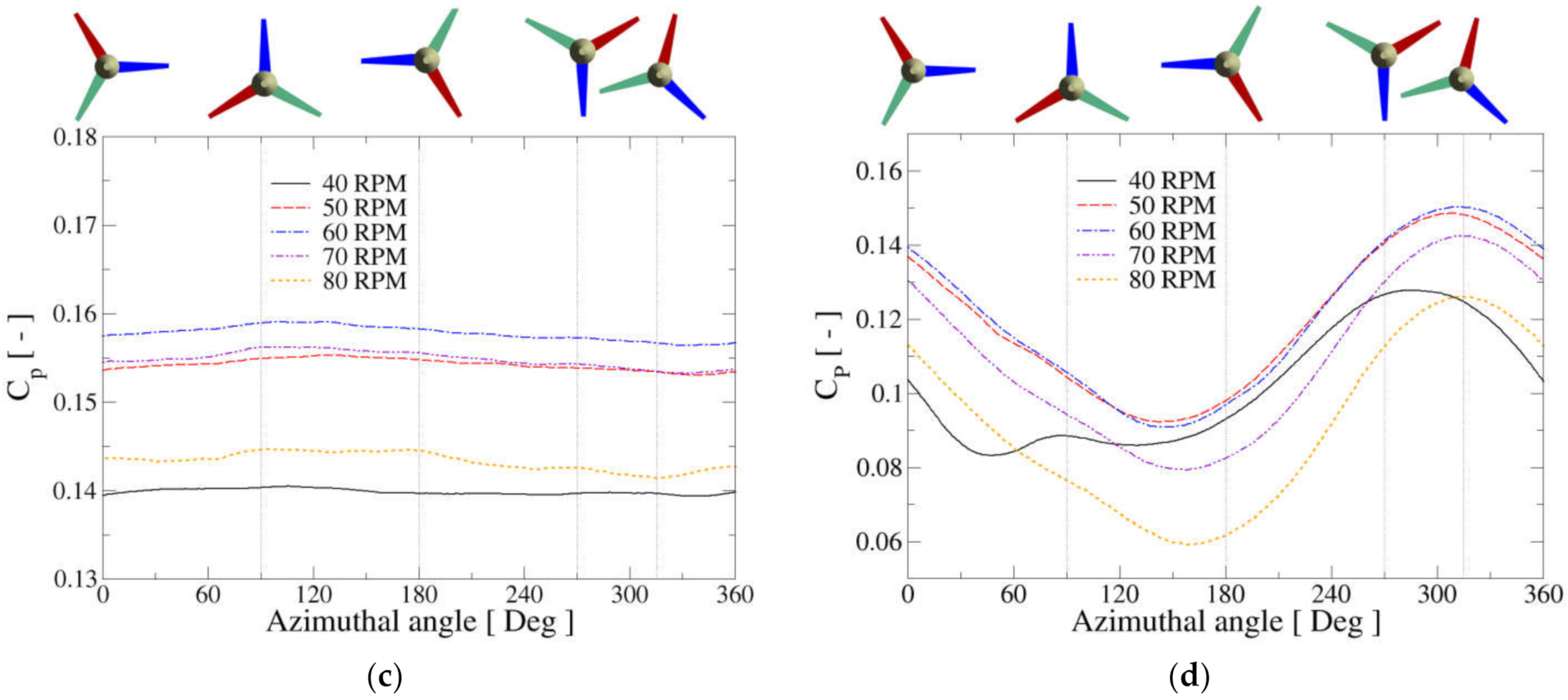
The behaviour of the coefficients for one blade is collected in Figure 8. The left column shows the coefficients for the PP configuration, and the right column for the TI arrangement. On the other hand, the upper row illustrates the thrust coefficient, while the power coefficient is presented in the lower row. As advanced, the thrust coefficient experienced by one blade in the PP turbine (Figure 8a) shows a constant value along the whole turn and increases with growing TSR, although not linearly. The power coefficient delivered for a single blade (Figure 8c) is also very approximately constant with , presenting its maximum for the angular velocity of 60 rpm; for lower and higher rotation rates, is reduced due to the stall phenomenon, in the former case, and low values of the effective flow angle of attack in the latter case. In both situations, the lift force experienced by the 2D profiles that compose the blade sections decreases, and therefore, the torque transferred to the blades by the fluid diminishes.
In the slanted turbine, both coefficients present an oscillatory evolution along a revolution, because the flow field seen in the blades changes along the azimuthal position, as mentioned previously. As in the PP turbine, the thrust coefficient increases with rotational speed (Figure 8b). The minimum value of is attained at , whereas the maximum appears around (Figure 8b). Above the plots, the positioning of the blades at certain angles is placed to visualise the location of blade one (in blue) at the points of interest. The position of the maximum is close to the point where the blade tip reaches the maximum depth, and it displaces towards higher angles as grows. For the curve presents clear minimum and maximum values where the first is at and the maximum at . However, for higher angular speeds, the blade shows in the upper half cycle (i.e., lower depth) a roughly flat behaviour of , while it is larger in the lower half cycle. On the other hand, the curves (Figure 8d) present distinguished maxima and minima, except for , where the curve shows two close minima at both sides of the azimuthal angle. For higher values of rotational speed, the curves are very similar with a slight displacement towards higher azimuthal angles as augments. In particular, the maximum power coefficient is located around and the minimum close to . Let us remark that the angular positions with higher value tend also to show a high thrust coefficient and vice versa.
Moreover, it is necessary to mention that in the inclined arrangement, in spite of that one-blade coefficients show a periodic behaviour, the full rotor coefficients have a flatter curve showing only a mild ripple [39]. This fact is due to the compensation of the contributions among the three blades.
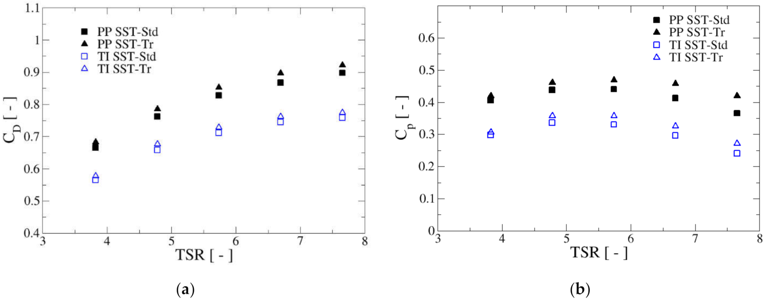
Figure 9 shows the thrust and power coefficients for the full turbine given by Equations (2) and (4) in both configurations, PP and TI. In this figure, the obtained results with the shear stress transport transitional turbulence model SST–Tr and those with the standard version SST–St are presented. As it can be readily seen from Figure 9a, the thrust coefficient on the PP configuration is higher than that of the TI disposition, which is likely a result of the narrower wake behind the rotor in the second case, a fact that reflects in a smaller pressure drag. Nevertheless, in the TI case, the blades experience alternating normal loads (see Figure 8b) which can cause material fatigue after long working periods. Moreover, the coefficient grows monotonically with TSR, although for TI, it seems that the curve approaches a plateau for the highest TSR values. These two facts are reproduced by both versions of the turbulence model; however, the transitional version provides somewhat higher values of than the standard one; the difference between both curves is roughly constant in the TI configuration but increases slightly in the PP setup.
Figure 9b presents the behaviour of the power coefficient for both arrangements and the two versions of the turbulence model. Similar to the thrust coefficient, is higher for the PP condition than for the tilted one, as is expected, because the available turbine cross-sectional area is larger in the first case. In addition, in the slanted turbine, the angle of attack of the flow seen in the blades changes along the azimuthal angle; the result is that the effective lift-to-drag ratio undergone by each blade is modified as it rotates, with the consequence that the net torque extracted from the fluid by the rotor diminishes. Finally, it is observed that the difference between the PP and TI values of augments as increases. The results also suggest that in the TI case, the location of the maximum is slightly displaced to a lower value of . Looking at the effects of the turbulence modelling, the transitional version predicts larger power coefficients than the standard version. This behaviour has been also found in previous works [22,29], and it indicates that the transference of energy from the water to the rotor is higher in the SST–Tr than in the standard version. In the next section, it is demonstrated that the real cause for such difference lies in the prediction of the wall shear stresses by both model versions. differences between such values grow as TSR increases for both, the PP and TI configurations, being the maximum discrepancy of 15% for PP and 12% for TI. In [22], using a vertical axis water turbine, a similar situation is found; there, the discrepancy between the results of transitional and standard versions is more than 40% for the highest computed value of . This fact indicates that the modelling of the boundary layer behaviour becomes crucial for increasing tip speed ratios in hydrokinetic turbines.
5. Analysis of the Influence of Boundary Layer Modelling on Turbine Performance
In this section, the detailed comparison of pressure and skin friction coefficients obtained by the two versions of the SST turbulence model is performed. Contour maps of such coefficients on the blades and 2D profiles of them at a certain span position on blade one are presented in the following figures. The pressure coefficient, , and skin friction coefficient, , are defined as follows:
In Equations (5) and (6), represents the static pressure and the magnitude of the wall shear stress vector.
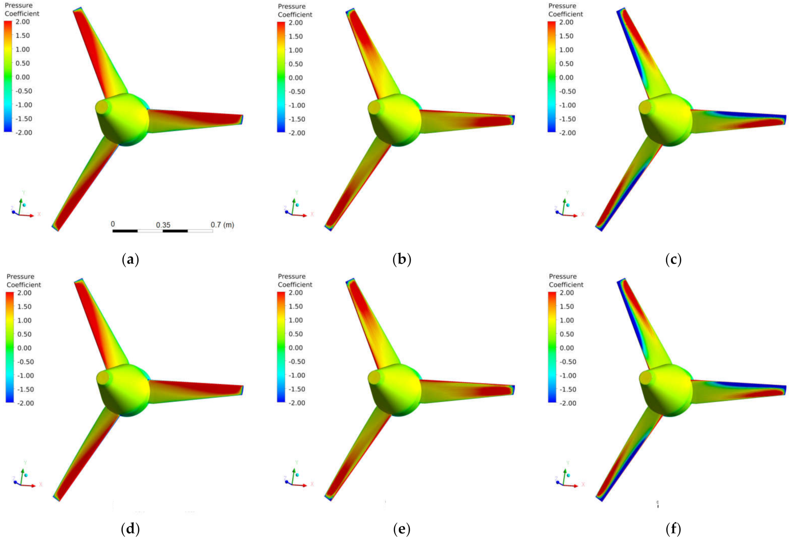
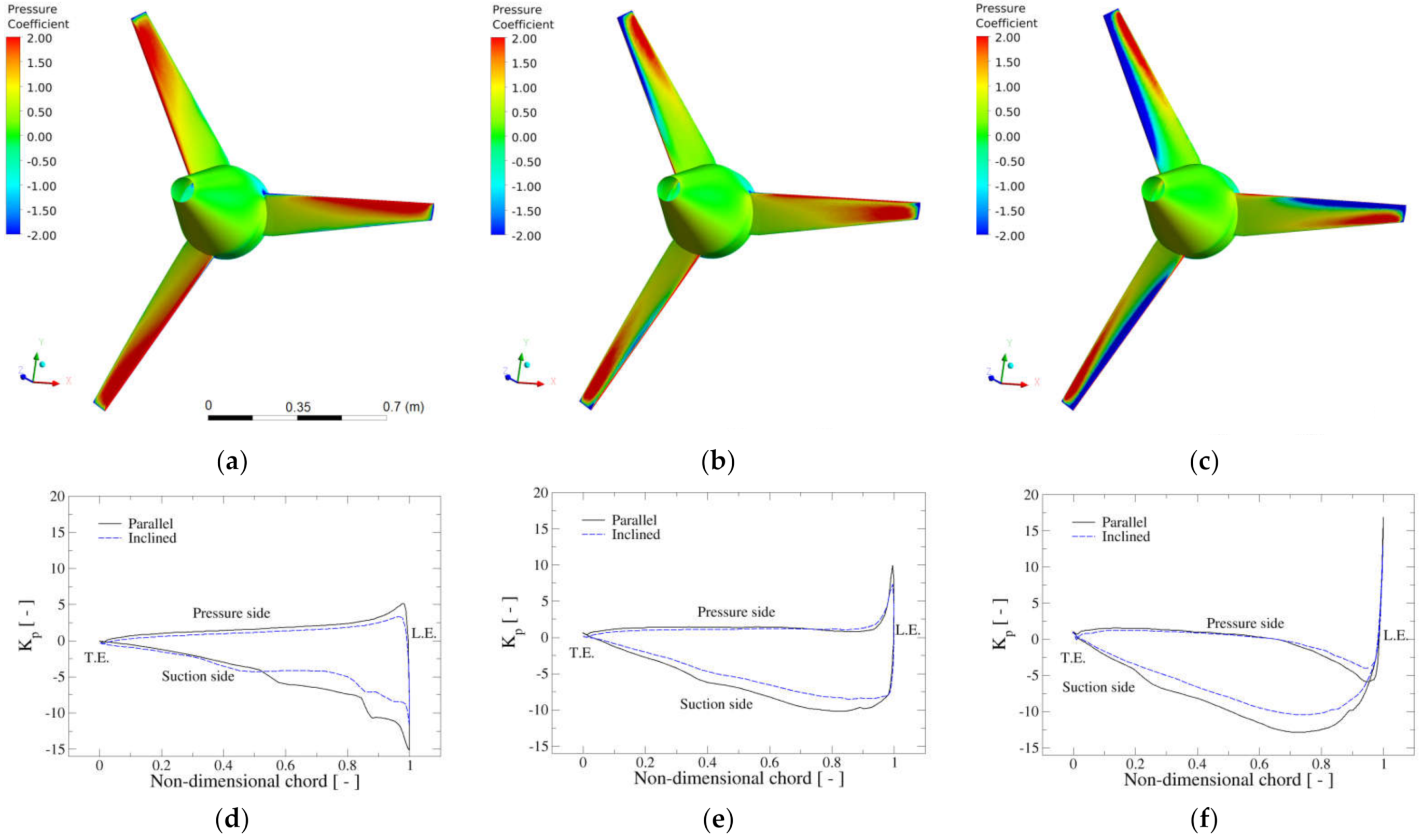
Figure 10 shows in isometric view the contour plot of on the pressure side of the blades for the rotational speeds and for the two versions of the turbulence model, SST–Tr (Figure 10a–c) and SST–St (Figure 10d–f), in the case of the PP configuration. The left column of this figure presents the results for , the middle for , and the right column for . Rotation is performed counterclockwise.
From Figure 10a–c, the dependence of with the TSR can be inferred. First of all, it can be readily seen that the pressure coefficient distribution on the three blades is basically the same. This fact has been commented on previously, and it owes to the equivalence of blades’ azimuthal position along its revolution in the PP turbine. In the case of (Figure 10a), shows positive values along the pressure side with values decreasing from the leading edge (LE) towards the trailing edge (TE); moreover, pressure coefficients are larger at blade tip than at the root. For (Figure 10b), the values of are still positive, but at cross sections from the midspan towards the blade tip, it is observed that the pressure coefficient presents a maximum at LE, then decreases to reach a local minimum and then grows slightly up to the mid chord for decreasing again towards the TE. In cross sections close to blade root, decreases continuously from LE to TE. When the angular speed is larger, (Figure 10c), negative values of pressure coefficient appear on the pressure side (blue color in the figure) which are located close to the LE at sections starting roughly from quarter span towards the blade tip. At the sections closer to the root, the positive values of are recovered along the whole chord.
Figure 10d–f displays the contour plots of pressure coefficient for the same rotor angular velocities computed with the standard version of the turbulence model. It can be readily observed that the distribution is very similar to that found with the SST–Tr version. In fact, looking at the 2D plots of this variable at the cross section located at midspan of the blade one at (Figure 11), it can be seen that the profiles of provided by both versions of the turbulence model lie one over the other nearly exactly for the three TSR. Only small differences are noticed in the suction side at some specific areas. Additionally, Figure 11a–c shows that the suction side of the blade always presents negative values of , except close to the LE at (Figure 11c) and that the peak value obtained at the leading edge increases with tip speed ratio. In summary, from Figure 10 and Figure 11, it can be concluded that both versions of the SST turbulence model provide essentially the same pressure coefficient distribution along the blades.
Figure 12 presents the results for the pressure coefficient in the case of the tilted turbine TI using the SST–Tr version of the turbulence model. The top row, Figure 11a–c, illustrates the contour plot of this variable along the blades for the three rotational speeds of (left), (middle), and (right). Regarding the contour plots, it can be inferred that the distribution is qualitatively similar to the PP configuration for the three considered rotational speeds. However, some differences can now be noticed between the contour plots on the three blades at each specific TSR; on this occasion, the inclination of the turbine causes that the flow field seen in the blade changes along its azimuthal angle. As a consequence, the maximum thrust is experienced by the blade around and the minimum around ; however, the exact value depends on the tip speed ratio, as it is shown in Figure 8b.
Same as happened with the PP configuration, the distribution along the blades of is nearly identical in the case of the two versions of the turbulence model, SST–Tr and SST–St; therefore, the results obtained for using the standard SST model are not shown.
Figure 12d–f shows the 2D curves for the midspan cross section of the first blade (SST–Tr version). In these plots, a comparison is made between the PP and TI configurations for the three rotational speeds considered. Qualitatively, the profiles of pressure coefficient are similar but some quantitative differences appear, especially in the suction side, where the slanted arrangement shows noticeably lower negative values than the PP configuration. This fact is responsible for the lower thrust and torque experienced in the former. On the other hand, on the pressure side, the curves are pretty close in both configurations although the values for TI are slightly lower than for the PP case.
Summarising the findings for the pressure coefficients, both versions of the turbulence model, standard and transitional, provide the same results so that the observed differences between their predictions of and are not due to the pressure distribution. Moreover, in the tilted turbine, the distribution along the blade depends on its azimuthal position. Overall, the pressure contribution to thrust and torque in TI configuration is lower than for the PP case.
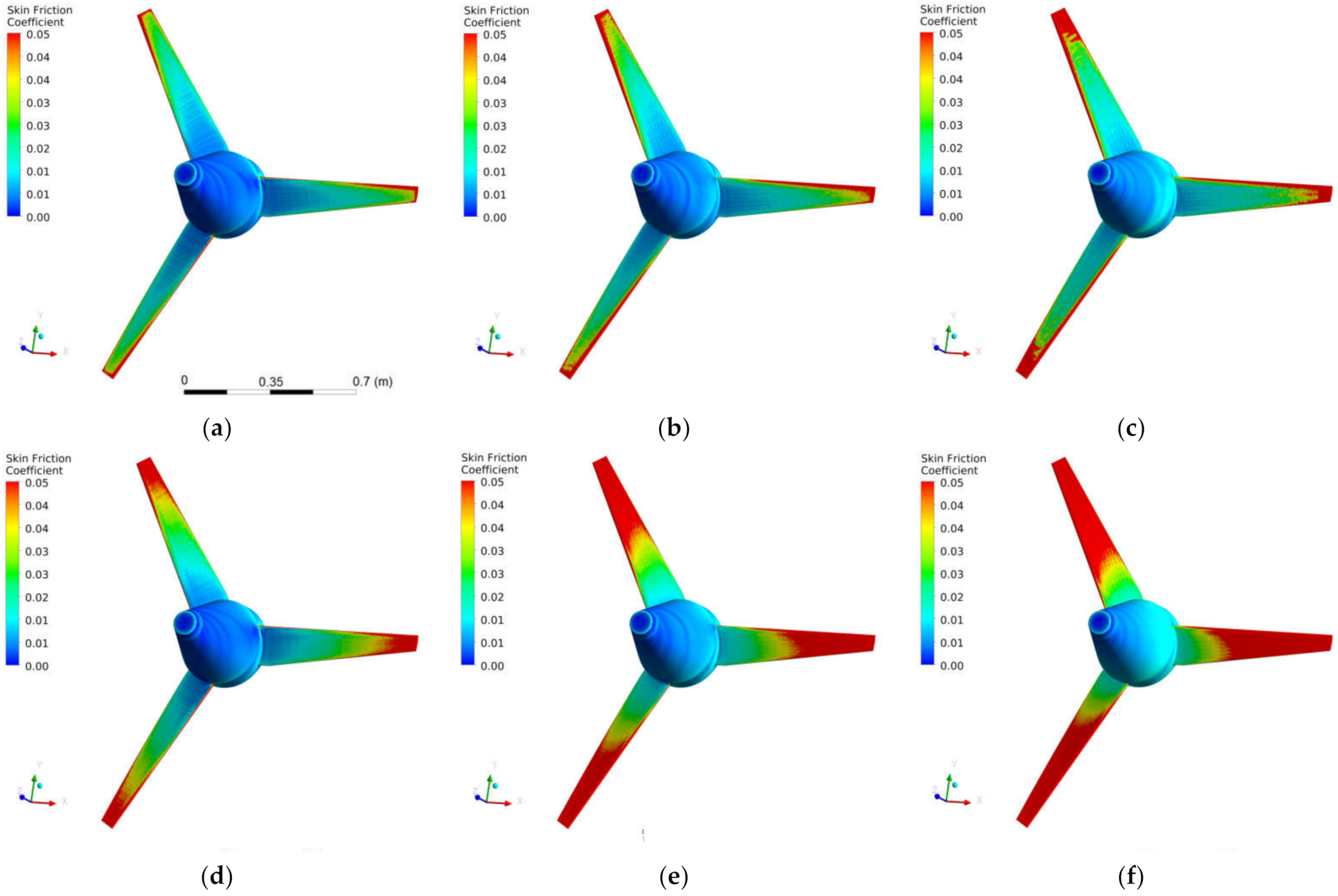
From now on, the behaviour of the skin friction coefficient is analysed depending on turbine inclination, tip speed ratio, and version of the employed turbulence model. Figure 13 presents the contours of the skin friction coefficient in the case of the PP turbine using the transitional version of the turbulence model (top row) and the corresponding standard formulation (bottom row). Again, the left column presents results for , the middle column for , and the right column for . Same as with the pressure coefficient, in the PP arrangement the contour plots of on the three blades are equivalent due to the existing symmetry of flow conditions regarding the azimuthal angle . The expected increase of friction coefficient values is obtained with growing rotational speed. The highest values are obtained in the leading edge at sections close to the blade tip; they decrease progressively towards the trailing edge, due to the development of the boundary layer, and towards the blade root, where the effective velocity seen in the blade is lower. Looking at the top and bottom rows, it is clearly demonstrated that the SST–St version of the turbulence model provides much higher values of skin friction coefficient than the transitional version, implying higher friction. Since friction forces always oppose the motion, the drag force acting on the blade increases, and the fluid torque (hence the power) transferred to the blade diminishes. The higher values of wall shear stresses generated by the SST–St model are the reason for the smaller predicted values of regarding the SST–Tr version.
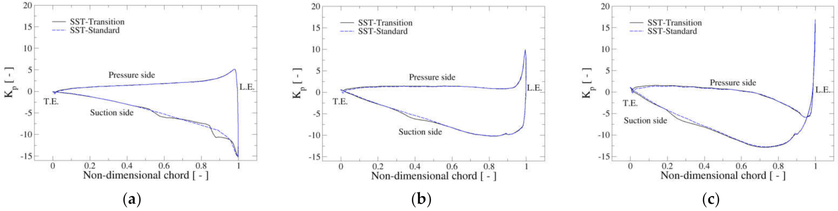
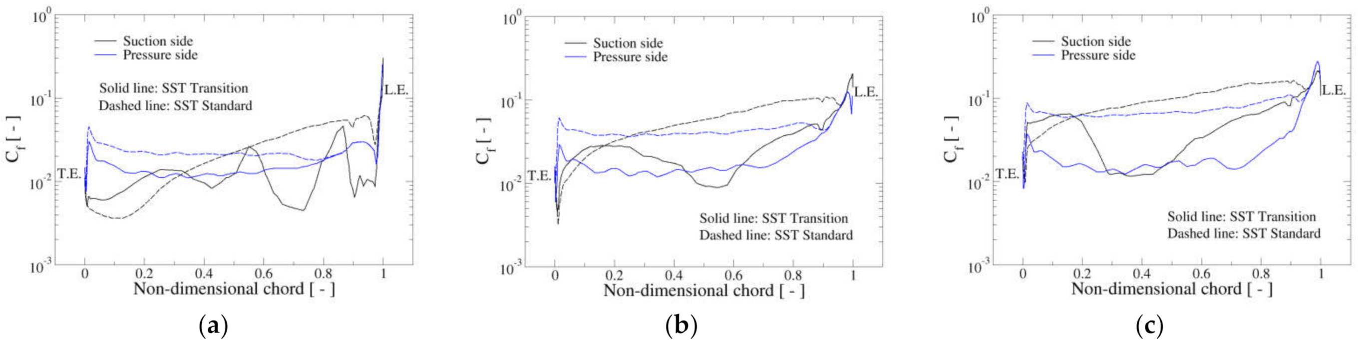
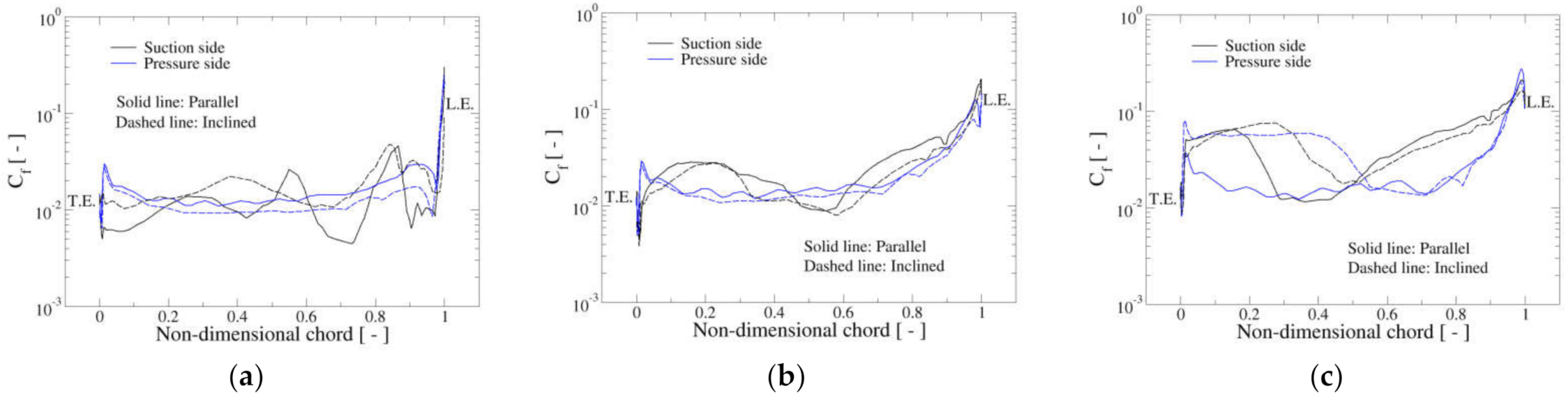
Profiles of comparing both versions of the SST turbulence model are provided in Figure 14 for the three considered rotor angular velocities at the midspan section of blade one at the azimuthal position . In Figure 14, solid lines represent SST–Tr values and dashed lines SST–St predictions. In the plots, it is readily seen how on the pressure side (blue lines) transitional model values are always much lower than those of the standard model (note the log scale in the y-axis). On the suction side, the SST–Tr curve shows the transition from laminar to turbulent boundary layer (identified here by a fast increase of the skin friction coefficient in points around the mid chord). This transition is nicely detected in the situation (Figure 14c), where the solid black curve rises suddenly from values of around 10−2 to 0.8 at the position of nondimensional chord . Additionally, on the suction side, the standard model wall shear stresses are usually larger than the corresponding values of the transitional formulation.
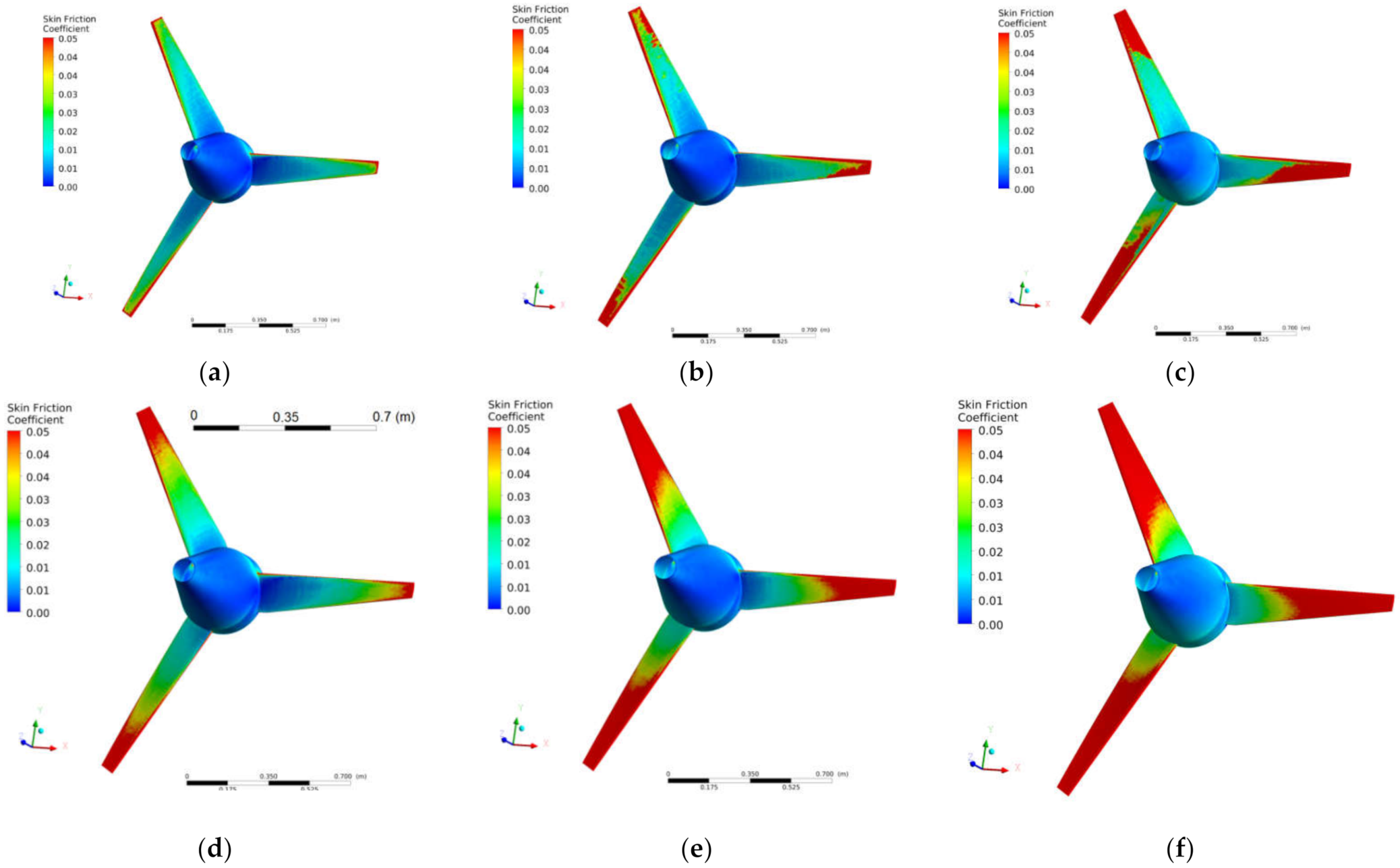
The behaviour of the skin friction coefficient in the tilted turbine, regarding the two formulations of the SST turbulence model, is pretty similar to the PP configuration, and it is presented in Figure 15. In this case, the distribution on the blades depends on the azimuthal angle, same as it was observed for the pressure coefficient. This is clearly illustrated by Figure 15c in which the red colors indicating high values are distributed in a different way in the three blades. Moreover, comparing with Figure 13, the extension of the red areas in the TI configuration is larger than for the PP turbine, which can be better seen in the case of the transitional model. Therefore, the blades in the inclined arrangement present lower pressure coefficients and larger skin friction coefficients than in the perpendicular rotor; both facts imply lower torque, hence power coefficient, in the former case.
Figure 16 compares the profiles for the PP and TI configurations at the midspan section of blade one at the azimuthal position . Computations are shown for the SST–Tr turbulence model. For the 40 and 60 angular speeds, values are quite comparable in both pressure and suction sides, showing some wiggles. For the case of , in the TI configuration, the transition from laminar to the turbulent boundary layer on the pressure side can be observed, but this is not observed for the PP arrangement. On the other hand, on the suction side, this transition is seen in both cases, but in the TI deployment, it happens earlier. As a result, the wall shear stresses are higher for the inclined than for the PP turbine.
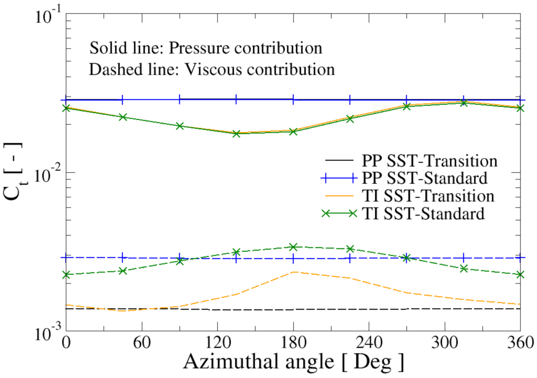
Additionally, Figure 17 presents the contribution to the full rotor torque coefficient of the pressure and viscous components along a complete revolution for both deployment configurations and the two turbulence model formulations at .
It can be observed from Figure 17 that the pressure contribution is around one order of magnitude larger than the viscous contribution. In this figure, it is seen that the pressure contribution to torque is exactly the same computed by the two versions of the turbulence model in the two configurations, PP and TI, during the complete revolution. However, the viscous contribution is noticeably higher for the SST–St version for the two turbine configurations. Let us remember that the viscous contribution always subtracts torque from the machine which highlights the reason why the SST–Tr version of the turbulence model provides a higher coefficients than the SST–St formulation. Additionally, the viscous contributions to in the PP and TI arrangements are comparable, meaning that the differences in the power transferred from the fluid to the rotor in them are mainly due to the pressure contribution which is higher in the PP turbine for all azimuthal positions.
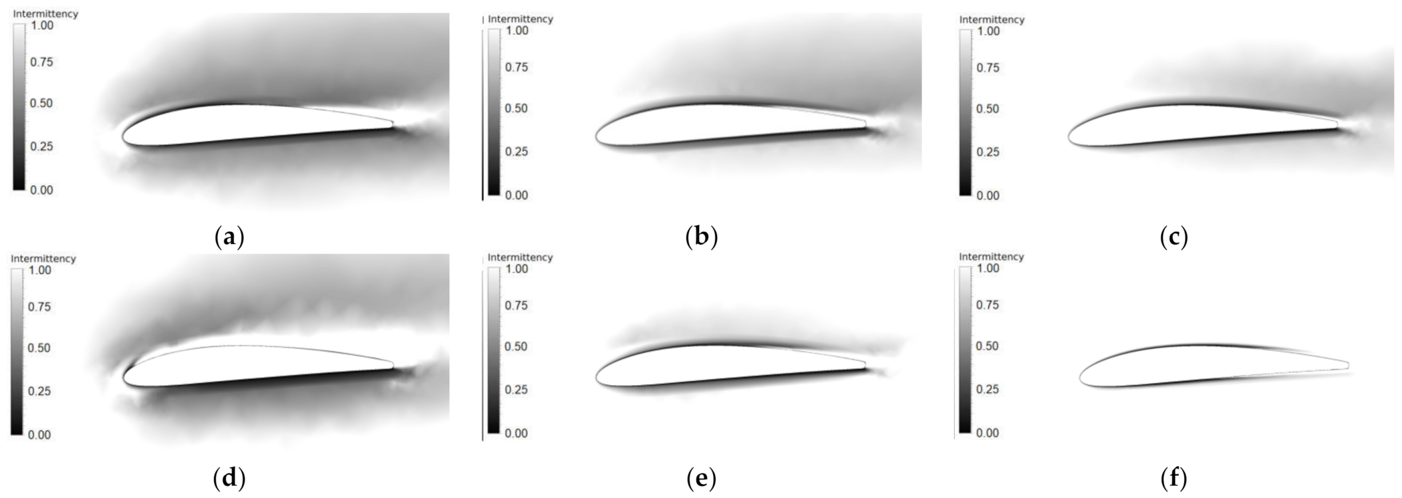
Finally, Figure 18 depicts the intermittency contour plots at a plane located at midspan of blade one at , for the two turbine arrangements and the three angular speeds rpm. The intermittency variable is computed in the SST transition turbulence model and represents in a point the fraction of time that the flow is turbulent. In Figure 18, values of intermittency of 0 correspond to fully laminar flow and values of 1 to fully turbulent flow. The upper row of such figure shows the results for the PP turbine at the three considered tip speed ratios. There, it can be observed that the size of the area of laminar flow around the blade (grey to black color) decreases as the TSR augments (compare Figure 18a–c). Moreover, the boundary layer along the pressure side remains laminar for the three values of but for the suction side, a point where intermittency changes suddenly from laminar to turbulent conditions is clearly distinguished. Of course, this feature is directly related to the transition from the laminar to the turbulent boundary layer.
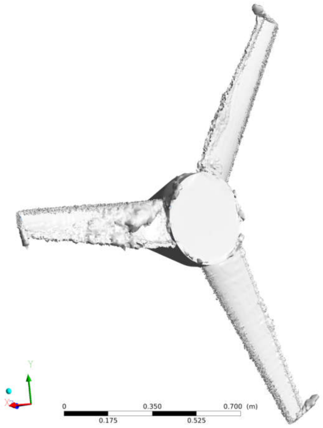
The respective intermittency contours for the tilted turbine are presented in the bottom row of Figure 18. As with the PP orientation, also the size of laminar flow areas around the blade is reduced as rotor speed increases; however, at 40 rpm (Figure 18d), the turbulent flow covers nearly all blade’s suction side, indicating the detachment of the boundary layer in this condition. This fact can be observed in Figure 19 by means of the isosurface of vorticity of , showing the uplift of such isosurface along half of the blade one span. On the other hand, laminar flow areas in Figure 18d–f are appreciably reduced when compared with those of the PP arrangement, indicating that turbulent flow conditions are more prevalent for the blades in the inclined turbine; of course, this fact reflects in a decrease in the torque transferred to the blades by the fluid. From Figure 18f, it can be inferred that the boundary layer experiences the transition from laminar to turbulent conditions in both sides of the blade, pressure and suction, and that the laminar region is confined to a very thin layer around the blade.
The obtained integral parameters for the Aquavatio turbine are compared in the following with some results of the literature. First of all, as it is shown in Figure 9b, the prediction of the optimal tip speed ratio is independent of the turbulence model. It is clear that for the PP configuration the maximum is achieved close to a TSR of 5.7, while in the TI configuration the maximum is located closer to 4.8. Of course, as it was pointed out, the magnitude of the power coefficient at these TSR depends on the turbulence model. Therefore, it is observed that the maximum is shifted to lower TSR and lower values as the angle of inclination of the turbine () increases. This reduction in (about 28%) is due to the increment in the angle of attack as increases; this fact is similar to an increment in the twist angle of the blade in which the same results are observed [40,41]. On the other hand, when comparing the present results (PP configuration) with the experimental results reported by Bahaj et al. (design case—5° set angle) [33], it is observed a good agreement n in the shape of the curve as well as in the maximum and position of the optimal TSR (). Additionally, [42] reported a similar shape of curve, with values of maximum and optimal TSR (between 4–6), when using upscaling laws from small-scale wind tunnel tests to full-size hydrokinetic turbines.
Finally, although the design improvement of the studied turbine was out of the scope of the present work, we can suggest several possibilities for increasing its performance. Firstly, the hydrodynamic design of the hub needs to be improved as the truncated cone geometry generates a wide wake behind it, consisting of a quasi-steady toroidal vortex that induces a backflow and low pressure in that zone. This wake increases the drag and reduces the power; therefore, the hub should be redesigned using a more aerodynamic shape aimed at reducing the turbine drag and increasing . To achieve this objective, it would be also useful to optimise the twist distribution along the blade span to avoid flow separation at the root. Additionally, it would be beneficial to use a different type of hydrofoil, for example, NACA 6 series, as in reference [33], together with an improved chord distribution and solidity.
6. Summary and Conclusions
This paper has addressed the CFD numerical simulation of an existing Garman-type HK turbine which was empirically designed and was in operation in the Cauca River, in the southwest of Colombia some years ago. However, the turbine was never experimentally characterised; therefore, their numerical simulation was the adopted alternative aimed to build its efficiency curve. The performed 3D transient simulations allowed analyzing the hydrodynamics of the flow around the turbine. The turbulent features of the flow were described by the SST turbulence model in two formulations: standard and transitional. The turbine operation has been analysed in the conditions of shaft parallel and inclined regarding the flow direction. The computed curve in the first condition has been compared with the results of classical BEM and potential methods showing similar trends, providing a maximum power coefficient slightly above 45%. The inclined turbine undergoes lower values of thrust coefficient than the parallel, but the is also lower with a maximum efficiency of around 35%. The obtained results indicate that the maximum of the efficiency curve tends to be displaced to lower values of as the inclination angle increases. Additionally, the blades in the slanted configuration experience alternating stresses that increase the fatigue of the material. Regarding the comparison of the two versions of the turbulence model, the transition SST formulation provides higher values of than its standard counterpart (6% at maximum efficiency); a fact that has been found previously in water turbines [22,29]. The reason for this discrepancy has been investigated in the present study examining the behaviour of the pressure and skin friction coefficients for all the computed tip speed ratios. The performed analysis demonstrates that the differences are caused by the higher predicted skin friction coefficient values in the case of the standard version of the SST turbulence model regarding the transition version. As a result, the friction torque increases with the effect of reducing the efficiency. Finally, intermittency contours at various rotational speeds have been presented, illustrating that the laminar flow region in the tilted turbine is substantially smaller than in the parallel configuration, especially for the highest computed tip speed ratio. This fact is also connected with the smaller efficiency of the inclined turbine regarding its PP counterpart.
As future work, the effects of the free surface modelling as well as the inclination angle on turbine performance will be investigated by coupling the volume of the fluid method with the sliding mesh technique.
Author Contributions
Conceptualisation, O.D.L. and S.L.; data curation, L.T.C.; formal analysis, O.D.L. and S.L.; funding acquisition, S.L. and O.D.L.; investigation, S.L. and L.T.C.; methodology, O.D.L. and S.L.; resources, S.L.; supervision, O.D.L. and S.L.; validation, L.T.C.; visualisation, L.T.C.; writing—review and editing, S.L. All authors have read and agreed to the published version of the manuscript.
Funding
This research was partially funded by the Young Researchers program from the Colombian Administrative Department of Science, Technology, and Innovation, Colciencias (Grant Number 0001635894) and partially by the Dirección de Investigaciones y Desarrollo Tecnológico of Universidad Autónoma de Occidente and Vicerrectoria de Investigaciones of Universidad de los Andes (Grant Number 16Inter-265). The APC was funded by Universidad Autónoma de Occidente.
Conflicts of Interest
The authors declare no conflict of interest. The funders had no role in the design of the study; in the collection, analyses, or interpretation of data; in the writing of the manuscript, or in the decision to publish the results.
References
- 2020 Hydropower Status Report, Sector Trends and Insights; International Hydropower Association: London, UK, 2020; Available online: https://hydropower-assets.s3.eu-west-2.amazonaws.com/publications-docs/2020_hydropower_status_report.pdf (accessed on 25 April 2021).
- Niebuhr, C.M.; van Dijk, M.; Neary, V.S.; Bhagwan, J.N. A review of hydrokinetic turbines and enhancement techniques for canal installations: Technology, applicability and potential. Renew. Sustain. Energy Rev. 2019, 113, 109240. [Google Scholar] [CrossRef]
- Güney, M.S.; Kaygusuz, K. Hydrokinetic energy conversion systems: A technology status review. Renew. Sustain. Energy Rev. 2010, 14, 2996–3004. [Google Scholar] [CrossRef]
- Kirke, B. Hydrokinetic and ultra-low head turbines in rivers: A reality check. Energy Sustain. Dev. 2019, 52, 1–10. [Google Scholar] [CrossRef]
- Quaranta, E. Stream water wheels as renewable energy supply in flowing water: Theoretical considerations, performance assessment and design recommendations. Energy Sustain. Dev. 2018, 45, 96–109. [Google Scholar] [CrossRef]
- Vermaak, H.J.; Kusakana, K.; Koko, P. Status of micro-hydrokinetic river technology in rural applications: A review of literature. Renew. Sustain. Energy Rev. 2014, 29, 625–633. [Google Scholar] [CrossRef]
- Loots, I.; van Dijk, M.; Barta, B.; van Vuuren, S.J.; Bhagwan, J.N. A review of low head hydropower technologies and applications in a South African context. Renew. Sustain. Energy Rev. 2015, 50, 1254–1268. [Google Scholar] [CrossRef] [Green Version]
- Kusakana, K.; Vermaak, H.J. Hydrokinetic power generation for rural electricity supply: Case of South Africa. Renew. Energy 2013, 55, 467–473. [Google Scholar] [CrossRef]
- Kirke, B. Hydrokinetic turbines for moderate sized rivers. Energy Sustain. Dev. 2020, 58, 182–195. [Google Scholar] [CrossRef]
- Laín, S.; Contreras, L.T.; López, O.D. A review on computational fluid dynamics modeling and simulation of horizontal axis hydrokinetic turbines. J. Braz. Soc. Sci. Eng. 2019, 41, 35. [Google Scholar] [CrossRef]
- Van Els, R.H.; Junior, A.C.P.B. The Brazilian experience with hydrokinetic turbines. Energy Procedia 2015, 75, 259–264. [Google Scholar] [CrossRef] [Green Version]
- Gaden, D. An Investigation of River Kinetic Turbines: Performance Enhancements, Turbine Modelling Techniques, and an Assessment of Turbulence Models. Master’s Thesis, University of Manitoba, Winnipeg, MB, Canada, 2007. [Google Scholar]
- Yang, B.; Shu, X. Hydrofoil optimization and experimental validation in helical vertical axis turbine for power generation from marine current. J. Ocean Eng. 2012, 42, 35–46. [Google Scholar] [CrossRef]
- Laín, S.; Aliod, R. Study on the Eulerian dispersed phase equations in non-uniform turbulent two-phase flows: Discussion and comparison with experiments. Int. J. Heat Fluid Flow 2000, 21, 374–380. [Google Scholar] [CrossRef]
- Laín, S.; García, J.A. Study of four-way coupling on turbulent particle-laden jet flows. Chem. Eng. Sci. 2006, 61, 6765–6785. [Google Scholar] [CrossRef]
- Laín, S.; Sommerfeld, M. A study of the pneumatic conveying of non-spherical particles in a turbulent horizontal channel flow. Braz. J. Chem. Eng. 2007, 24, 535–546. [Google Scholar] [CrossRef] [Green Version]
- Mannion, B.; Leen, S.; Nash, S. A two and three-dimensional CFD investigation into performance prediction and wake characterisation of a vertical axis turbine. J. Renew. Sustain. Energy 2018, 10, 034503. [Google Scholar] [CrossRef]
- Laín, S.; García, M.; Orrego, S.; Quintero, B. CFD Numerical simulations of Francis turbines | Simulación numérica (CFD) de turbinas Francis. Rev. Fac. Ing. Univ. Antioq. 2010, 51, 24–33. [Google Scholar]
- Teran, L.A.; Rodríguez, S.A.; Laín, S.; Jung, S. Interaction of particles with a cavitation bubble near a solid wall. Phys. Fluids 2018, 30, 123304. [Google Scholar] [CrossRef] [Green Version]
- Sommerfeld, S.; Laín, S. Parameters influencing dilute-phase pneumatic conveying through pipe systems: A computational study by the Euler/Lagrange approach. Can. J. Chem. Eng. 2015, 93, 1–17. [Google Scholar] [CrossRef]
- Delafin, P.L.; Nishino, T.; Kolios, A.; Wang, L. Comparison of low-order aerodynamic models and RANS CFD for full scale vertical axis wind turbines. Renew. Energy 2017, 109, 564–575. [Google Scholar] [CrossRef] [Green Version]
- Marsh, P.; Ranmuthugala, D.; Penesis, I.; Thomas, G. The influence of turbulence model and two and three-dimensional domain selection on the simulated performance characteristics of vertical axis tidal turbines. Renew. Energy 2017, 105, 106–116. [Google Scholar] [CrossRef]
- Al-Dabbagh, M.; Yuce, M. Numerical evaluation of helical hydrokinetic turbines with different solidities under different flow conditions. Int. J. Environ. Sci. Technol. 2019, 16, 4001–4012. [Google Scholar] [CrossRef]
- López, O.; Meneses, D.; Quintero, B.; Laín, S. Computational study of transient flow around Darrieus type cross flow water turbines. J. Sust. Ren. Energy 2016, 8, 014501. [Google Scholar] [CrossRef]
- Chiroque, J.; Dávila, C. Microaerogenerador IT-PE-100 Para Electrificación Rural; Soluciones Prácticas-ITDG: Lima, Perú, 2012. (In Spanish) [Google Scholar]
- Menter, F.R. Zonal two equation k-turbulence models for aerodynamic flows. In Proceedings of the 23rd Fluid Dynamics, Plasmadynamics, and Lasers Conference, Orlando, FL, USA, 6–9 July 1993. [Google Scholar]
- Menter, F.R. Two-equation eddy-viscosity turbulence models for engineering applications. AIAA J. 1994, 32, 269–289. [Google Scholar] [CrossRef] [Green Version]
- Langtry, R.B.; Menter, F.R. Correlation-based transition modeling for unstructured parallelized computational fluid dynamics codes. AIAA J. 2009, 47, 2894–2906. [Google Scholar] [CrossRef]
- Laín, S.; Taborda, M.A.; López, O.D. Numerical study of the effect of winglets on the performance of a straight blade Darrieus water turbine. Energies 2018, 11, 297. [Google Scholar] [CrossRef] [Green Version]
- Salunkhe, S.; El Fajri, O.; Bhushan, S.; Thompson, D.; O’Doherty, D.; O’Doherty, T.; Mason-Jones, A. Validation of Tidal Stream TurbineWake Predictions and Analysis of Wake Recovery Mechanism. J. Mar. Sci. Eng. 2019, 7, 363. [Google Scholar] [CrossRef] [Green Version]
- Guillaud, N.; Balarac, G.; Goncalves, E.; Zanette, J. Large Eddy Simulations on Vertical Axis Hydrokinetic Turbines -Power coefficient analysis for various solidities. Renew. Energy 2020, 147, 473–486. [Google Scholar] [CrossRef] [Green Version]
- Laín, S.; Cortés, P.; López, O.D. Numerical Simulation of the Flow around a Straight Blade Darrieus Water Turbine. Energies 2020, 13, 1137. [Google Scholar] [CrossRef] [Green Version]
- Bahaj, A.S.; Batten, W.M.J.; McCann, G. Experimental verifications of numerical predictions for the hydrodynamic performance of horizontal axis marine current turbines. Renew. Energy 2007, 32, 2479–2490. [Google Scholar] [CrossRef]
- Wu, H.; Chen, L.; Yu, M.; Li, W.; Chen, B. On design and performance prediction of the horizontal axis water turbine. Ocean Eng. 2012, 50, 23–30. [Google Scholar] [CrossRef]
- Marten, D.; Wendler, J.; Pechlivanoglou, G.; Nayeri, C.N.; Paschereit, C.O. Qblade: An open source tool for design and simulation of horizontal and vertical axis wind turbines. Int. J. Emerg. Technol. Adv. Eng. 2013, 3, 264–269. [Google Scholar]
- Lee, J.H.; Park, S.; Kim, D.H.; Rhee, S.-H.; Kim, M.C. Computational methods for performance analysis of horizontal axis tidal stream turbines. Appl. Energy 2012, 98, 512–523. [Google Scholar] [CrossRef]
- Yuce, M.I.; Muratoglu, A. Hydrokinetic energy conversión systems: A technology status review. Renew. Sustain. Energy Rev. 2015, 43, 72–82. [Google Scholar] [CrossRef]
- QBlade v0.95—Guidelines for Lifting Line Free Vortex Wake Simulations. Available online: https://goo.gl/htvb34 (accessed on 22 August 2020).
- Contreras, L.T.; López, O.D.; Laín, S. Computational Fluid Dynamics Modelling and Simulation of an Inclined Horizontal Axis Hydrokinetic Turbine. Energies 2018, 11, 3151. [Google Scholar] [CrossRef] [Green Version]
- Kolekar, N.; Banerjee, A. A coupled hydro-structural design optimization for hydrokinetic turbines. J. Renew. Sustain. Energy 2013, 5, 053146. [Google Scholar] [CrossRef] [Green Version]
- Rares-Andrei, C.; Florentina, B.; Gabriela, O.; Lucia-Andreea, E. Power prediction method applicable to horizontal axis hydrokinetic turbines. In Proceedings of the International Conference on Energy and Environment (CIEM), Bucharest, Romania, 19–20 October 2017; pp. 221–225. [Google Scholar]
- Macias, M.M.; Mendes, R.C.F.; Oliveira, T.F.; Brasil, A.C.P., Jr. On the upscaling approach to wind tunnel experiments of horizontal axis hydrokinetic turbines. J. Braz. Soc. Mech. Sci. Eng. 2020, 42, 539. [Google Scholar] [CrossRef]
Figure 1.
Photographs of the Aquavatio turbine: (a) detail of the rotor with hub and blades; (b) barge with the turbine in operation in the Cauca River; notice the axis inclination angle. (Images courtesy of Aprotec).
Figure 1.
Photographs of the Aquavatio turbine: (a) detail of the rotor with hub and blades; (b) barge with the turbine in operation in the Cauca River; notice the axis inclination angle. (Images courtesy of Aprotec).

Figure 2.
Illustration of the operating conditions of the Aquavatio turbine, showing its components.
Figure 2.
Illustration of the operating conditions of the Aquavatio turbine, showing its components.

Figure 3.
Computational domain showing the main boundary conditions.

Figure 4.
Illustration of the surface mesh on the rotor and shaft.

Figure 5.
Comparison of the present CFD computations with the reference experiments of [31].
Figure 5.
Comparison of the present CFD computations with the reference experiments of [31].

Figure 6.
Comparison of the present CFD results with those obtained with simplified methods implemented in the software Qblade. Results for the PP configuration and the SST–Tr turbulence model.
Figure 6.
Comparison of the present CFD results with those obtained with simplified methods implemented in the software Qblade. Results for the PP configuration and the SST–Tr turbulence model.

Figure 7.
Illustration of the rotor reference system. Blades rotate counterclockwise.

Figure 8.
Evolution of the power and thrust coefficients experienced by blade one (in blue) along a turn for the PP configuration (left column) and TI configuration (right column): (a,b) thrust coefficient; (c,d) power coefficient.
Figure 8.
Evolution of the power and thrust coefficients experienced by blade one (in blue) along a turn for the PP configuration (left column) and TI configuration (right column): (a,b) thrust coefficient; (c,d) power coefficient.


Figure 9.
Thrust (a) and power (b) coefficients as a function of the tip speed ratio for the two turbine arrangements: PP (full symbols) and TI (hollow symbols). Additionally, computations with the standard (squares) and transitional (triangles) versions of the SST turbulence model are included.
Figure 9.
Thrust (a) and power (b) coefficients as a function of the tip speed ratio for the two turbine arrangements: PP (full symbols) and TI (hollow symbols). Additionally, computations with the standard (squares) and transitional (triangles) versions of the SST turbulence model are included.

Figure 10.
Pressure coefficient contour plots for the PP turbine at Top row shows the results for the transitional SST–Tr version and bottom row for the standard SST–St version of the turbulence model. From left to right the graphics correspond to rotor angular velocities of , , and , respectively.
Figure 10.
Pressure coefficient contour plots for the PP turbine at Top row shows the results for the transitional SST–Tr version and bottom row for the standard SST–St version of the turbulence model. From left to right the graphics correspond to rotor angular velocities of , , and , respectively.

Figure 11.
Comparison of the distribution along the chord of first blade at midspan for the two versions of the turbulence model, SST–Tr, and SST–St. From left to right the graphics correspond to rotor angular velocities of rpm (a), rpm (b) and (c). PP configuration at .
Figure 11.
Comparison of the distribution along the chord of first blade at midspan for the two versions of the turbulence model, SST–Tr, and SST–St. From left to right the graphics correspond to rotor angular velocities of rpm (a), rpm (b) and (c). PP configuration at .

Figure 12.
Pressure coefficient distribution for the TI turbine. Top row shows the contour plots for the transitional SST–Tr version. Bottom row displays the distribution along the chord of first blade at at midspan for both operating conditions of the turbine: rotor perpendicular to the flow (PP) and tilted (TI). From left to right the graphics correspond to rotor angular velocities of , , and , respectively.

Figure 13.
Skin friction coefficient contour plots for the PP turbine. Top row shows the results for the transitional SST–Tr version and bottom row for the standard SST–St version of the turbulence model. From left to right the graphics correspond to rotor angular velocities of , and , respectively.

Figure 14.
Comparison of the distribution along the chord of first blade at midspan at for the two versions of the turbulence model, SST–Tr and SST–St. From left to right the graphics correspond to rotor angular velocities of rpm (a), rpm (b) and (c), respectively. PP configuration.
Figure 14.
Comparison of the distribution along the chord of first blade at midspan at for the two versions of the turbulence model, SST–Tr and SST–St. From left to right the graphics correspond to rotor angular velocities of rpm (a), rpm (b) and (c), respectively. PP configuration.

Figure 15.
Skin friction coefficient contour plots for the TI turbine. Top row shows the results for the transitional SST–Tr version and bottom row for the standard SST–St version of the turbulence model. From left to right the graphics correspond to rotor angular velocities of , and , respectively.

Figure 16.
Comparison of the distribution along the chord of first blade at midspan at for the PP and TI configurations. From left to right the graphics correspond to rotor angular velocities of rpm (a), rpm (b) and (c), respectively. SST–Tr model.
Figure 16.
Comparison of the distribution along the chord of first blade at midspan at for the PP and TI configurations. From left to right the graphics correspond to rotor angular velocities of rpm (a), rpm (b) and (c), respectively. SST–Tr model.

Figure 17.
Contribution to torque coefficient of pressure and viscous components in the studied cases at .
Figure 17.
Contribution to torque coefficient of pressure and viscous components in the studied cases at .

Figure 18.
Intermittency contour plots at midspan of blade one at obtained with the SST–Tr version of the turbulence model. Top row shows the results for the PP turbine and bottom row for the TI arrangement. From left to right the graphics correspond to rotor angular velocities of , , and , respectively.

Figure 19.
Illustration of boundary layer detachment at by means of the geometry of the vorticity isosurface.
Figure 19.
Illustration of boundary layer detachment at by means of the geometry of the vorticity isosurface.

Publisher’s Note: MDPI stays neutral with regard to jurisdictional claims in published maps and institutional affiliations. |
© 2021 by the authors. Licensee MDPI, Basel, Switzerland. This article is an open access article distributed under the terms and conditions of the Creative Commons Attribution (CC BY) license (https://creativecommons.org/licenses/by/4.0/).
Share and Cite
MDPI and ACS Style
Laín, S.; Contreras, L.T.; López, O.D. Hydrodynamic Characterisation of a Garman-Type Hydrokinetic Turbine. Fluids 2021, 6, 186. https://0-doi-org.brum.beds.ac.uk/10.3390/fluids6050186
AMA Style
Laín S, Contreras LT, López OD. Hydrodynamic Characterisation of a Garman-Type Hydrokinetic Turbine. Fluids. 2021; 6(5):186. https://0-doi-org.brum.beds.ac.uk/10.3390/fluids6050186
Chicago/Turabian StyleLaín, Santiago, Leidy T. Contreras, and Omar D. López. 2021. "Hydrodynamic Characterisation of a Garman-Type Hydrokinetic Turbine" Fluids 6, no. 5: 186. https://0-doi-org.brum.beds.ac.uk/10.3390/fluids6050186