
Evaluation of Magnus Force on Check Ball Behavior in a Hydraulic L Shaped Pipe


Department of Mechanical Engineering, Faculty of Science and Engineering, Kindai University, Higashiosaka 577-8502, Osaka, Japan
Fluids 2021, 6(5), 191; https://0-doi-org.brum.beds.ac.uk/10.3390/fluids6050191
Submission received: 16 April 2021
/
Revised: 11 May 2021
/
Accepted: 17 May 2021
/
Published: 19 May 2021
(This article belongs to the Special Issue Modelling the Behaviour of Water Systems to Increase Sustainability)
Abstract
:This paper presents the effect of the rotational speed of a check ball in a hydraulic L-tube on the translational motion caused by the Magnus effect. A spring-driven ball check valve is one of the most important components of a hydraulic system and controls the position of the ball to prevent backflow. To simplify the structure, the springs must be eliminated. To this end, it is necessary to clarify the flow pattern of the check ball in an L-shaped pipe and the rotational and translational behaviors of the ball. In this study, the position of the inlet pipe and the availability of the check were determined using Computer Aided Engineering (CAE) tools. By moving the position of the inlet pipe from the top to the bottom of the housing, the direction of the rotation of the ball was reversed, and the behavior changed significantly. It was found that the Magnus force, which causes the ball to levitate by rotating it in the opposite direction to the flow, acts to shorten the floating time.
1. Introduction
Hydraulic systems are used for work that requires linear and rotational motion, large forces, and freely changeable speed. The advancement of hydraulic technology has allowed the use of hydraulic systems as a means of energy transfer not only in construction and civil engineering equipment but also in products that are more closely associated with people’s daily lives, such as automobiles, airplanes, and elevators. One of the important components of a hydraulic system is the check valve. Generally, most check valves that use a ball also use a spring to push the ball and regulate its position to reliably prevent back flow. However, there is a strong need to eliminate the spring because it brakes by the chattering of the ball, and also to reduce the cost. Additionally, the piping shapes used around the check valve are the straight type and L-shaped elbow type. Tests and analytical research on the shape of straight-type check valves have been conducted [1,2]. Furthermore, eigenvalue analysis, three-dimensional numerical analysis, and so on, have been conducted on poppet valves [3]. A simulation method for fluid power systems has been developed, and several detailed analysis results have been obtained by comparing the simulation results to actual measurement results [4]. Moreover, comprehensive reviews of flow-induced vibrations have been reported by many studies [5,6,7,8,9].
The check ball behavior of hydraulic check valves with L-shaped piping in terms of the hydraulic fluid flow, the effect on the check ball behavior of that flow, and so on, has not been clarified to date. The flow in the pipe applies a hydrodynamic force to the ball, which causes the flow around the check ball to become more complex and perpendicularly bend further. At this time, the behavior of the check ball is subject to the complex relationship between the flow path’s relative position and the flow rate, viscosity, and other factors.
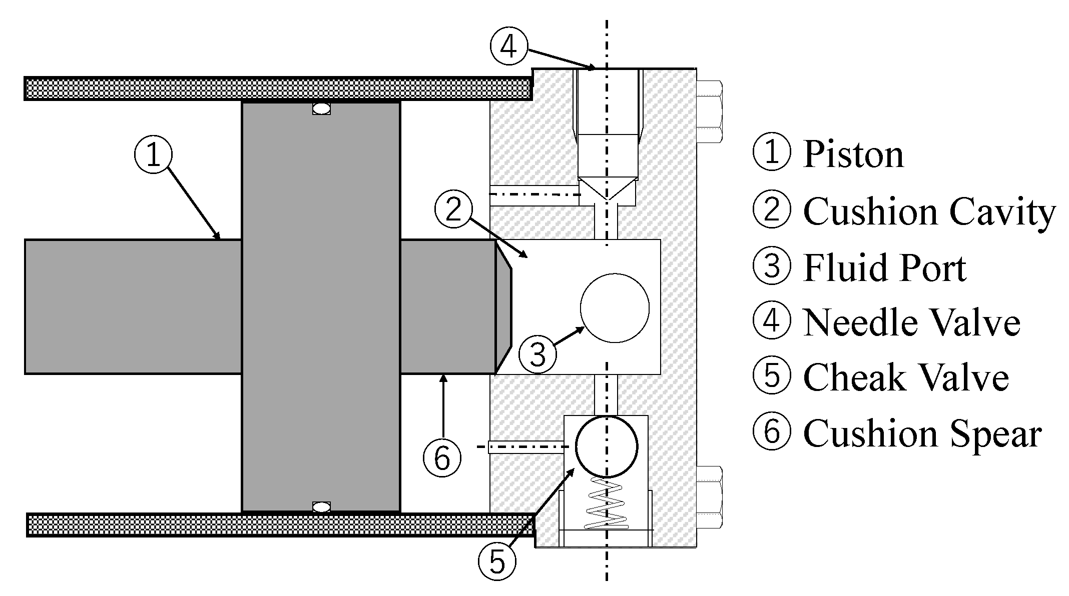
An example on the use of the check ball of the hydraulic check valves with L-shaped piping is shown in Figure 1. The cushions are small diameter pistons (6) entering a small cavity (2) machined into the end caps. The cylinder heads with cushions typically have a built-in check valve (5), which allows the free flow of hydraulic fluid into the cylinder such that the speed of the cylinder is not limited when the travel direction is reversed. Cylinders with adjustable cushions have needle valves (4) mounted onto the heads such that the fluid flow leaving the cushion can be adjusted and the amount of deceleration can be tuned to a particular application.
The behavior of the check ball of a hydraulic check valve with L-shaped piping has been experimentally observed, and the relationship between the check flow rate and the viscosity [10], the relationship between the ball and the inlet position [11], and so on, have been elucidated. However, the flow of the working fluid in a hydraulic check valve with L-shaped piping and the effect of the flow on the behavior of the check valve have not been clarified to date. The flow in the piping exerts a hydrodynamic force on the check ball, and the flow around the check ball becomes complex and further bends in a right-angle direction. At this time, the behavior of the check ball depends on the complex relationship between the relative position of the flow path, flow velocity, and viscosity. Because the rotation of the ball also affects the flow, and the rotational force on the ball changes with the flow, it is important to investigate the effect and influence of the CAE. The check ball should be operated under low-flow conditions. When the check ball is rotated by the flow, the lift force caused by the Magnus effect may reduce the flow rate. The force caused by the Magnus effect in uniform flow can be calculated using the Kutta–Zhukovsky theorem, as follows [12]:
where ρ is the working fluid density and U is the flow velocity; Γ represents the circulation and is expressed as follows:
Equations (1) and (2) express that the Magnus force changes with the flow velocity and the vortex strength. However, because these equations assume uniform flow, rotational motion is also included because the direction of the main flow in the L-shaped pipe can change by 90° and the flow is complicated by the position and movement of the check ball. The behavior of the check ball, its acting force, and the detailed fluid flow in the pipe have not been clarified. In this study, CAE analysis was carried out to clarify the flow of hydraulic fluid in L-shaped piping and the effects of the rotational and linear motions of the ball caused by the fluid. In this CAE analysis, the mutual influence of the ball motion and flow were confirmed using a polymerized grid. The effect of rotation was clarified by comparing the analysis results for the case wherein the ball motion has six degrees of freedom to the analysis results for the case wherein the ball motion has three degrees of freedom and can only perform translation without rotation.
2. Numerical Simulation
2.1. Governing Equations
In this paper, the dynamics of the flow in an L-shaped pipe is discussed. On average, the Reynolds number is small, but a low-Reynolds-number type turbulence AKN model [13] is used to deal with local increases. The flow of hydraulic fluid is governed by the conservation of mass equation (continuity equation) and the momentum equation (Navier–Stokes equation). For incompressible flow, a two-equation RANS approach based on the continuity equation, three momentum equations, and two transport equations is adopted. With xi being the coordinate axis in the i-direction, the time-averaged continuity and momentum equations (Navier–Stokes equations) can be written as:
where the symbols Ui, P, μ, and ρ represent the i-components of velocity, pressure, kinematic viscosity, and density, respectively; δij and are the Kronecker delta and body forces; and Sij is the rate of the average strain tensor defined as:
The additional term in Equation (4) is known as the Reynolds stress term and is attributed to the field due to the fluctuating velocity field. To close the nonlinear Reynolds stress term, additional modeling is required. The k-ε model uses two additional transport equations to solve the fluid problem. One is the turbulent kinetic energy, denoted by k, and the other is the dissipation rate of the turbulent kinetic energy, denoted by ε. Here, the following Abe–Kondoh–Nagano low-Re k-ε (AKN) model is used [13]. The AKN model is shown to work well with low-Reynolds-number complex flows. The AKN model achieves feasibility through turbulence time scales. The main improvement of the AKN is the usage of the Kolmogorov velocity scale uη, , instead of the friction velocity, , to account for the near-wall and low-Reynolds-number effects in the attached and detached flows [13], where is the shear stress at the wall. A low-Reynolds-number approach is adopted by applying a damping function to the layers affected by viscosity (viscous lower layer, buffer layer, and overlap region). The transport equations and algebraic relations relevant to the AKN model are given below.
where:
In Equation (8), vt is the turbulent eddy viscosity in the AKN model and is defined as:
The damping functions, fμ and fε, are defined below; fμ is referred to as the damping function and is required to be incorporated into the wall effect and the eddy viscosity coefficient. Because strong viscous stress action and turbulence damping action occur in the near-wall region, terms are added to reproduce these effects.
where:
and the normalized wall distance, y+, is defined as:
2.2. Meshing Method
A method called Arbitrary Lagrangian Eulerian (ALE) has been proposed to handle the flow around a moving object [14]. This is a method of moving a mesh, where the effect of moving the mesh is added to the equation of the static coordinate system. The L-shaped housing is meshed in a static coordinate system, and the area around the ball is meshed separately in a moving coordinate system. In the mass conservation Equation (3) and the momentum conservation Equation (4), Ui is replaced with (Ui − Wi) in the calculation. Ui must also be replaced by (Uj − Wj) for the equation of conservation of energy, turbulent energy, and turbulent loss rate (k–ε equation). Here, the added Wi denotes the moving velocity of the mesh. It should be noted that all variables appearing here are using values seen in a stationary coordinate system. In order to perform a coupled analysis of flow and object motion, the motion of the object is calculated based on the equations of motion of the dynamics and the moving speed of the element movement is set accordingly. The object is considered to be a rigid body, and the motion with six degrees of freedom is solved. The equations of motion for translation (the basic equations of Newtonian mechanics) and rotation are solved.
F is force, M is the mass of the check ball, V is the velocity of the check ball, and t is time. The subscript i represents the vector component in the Cartesian coordinate basis. Ffl is the force exerted by the surrounding fluid on the object, and the solver calculates this value. Fg is the gravitational acceleration, which also acts on the object in the direction of gravity.
Using the rotational speed, moment of inertia, I, and moment of force (torque), Ti, the equation of motion can be expressed as follows:
This gives the pressure-viscous torque, Ti, of the fluid acting on the surface of the object. This Ti is the torque exerted by the surrounding fluid on the object, and the solver calculates this value.
2.3. CAE Analysis Method
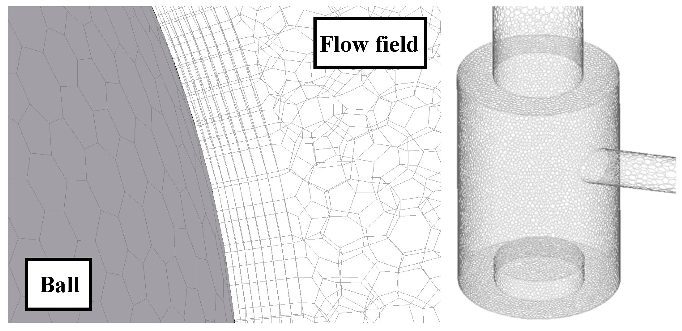
The thermofluid CAE analysis tool SCRYU/Tetra was used for analysis, and the state of the flow was observed. A low Re k–ε model was used for the turbulent flow model, and a no-slip condition was used for the wall surface condition. Figure 2 shows an example of the mesh arrangement. Eight layers with a 1.5 × 10⁻⁴ m-thick boundary layer mesh were inserted to improve the resolution of the separation and reattachment in the vicinity of the wall surface. The mass flow rate specification was considered for the inflow condition, and the natural inflow and outflow conditions were considered for the outflow condition. For the mesh preparation, the area from the inflow opening to the vicinity of the ball was very carefully observed, and a steady analysis was conducted using a mesh partition number of approximately eight million. The area around the ball was also divided into approximately three million meshes, and CAE analysis was carefully carried out using the polymerized grid method. Of course, the finer the mesh, the more accurate the response. A mesh independence has also been conducted to determine the dependence of the results on the mesh density. The mesh density was carefully determined based on analysis time and analytical judgment of the results. In particular, the surface of the ball was divided into very dense meshes because of the changes in the flow due to the rotation of the ball.
2.4. CAE Analysis Models
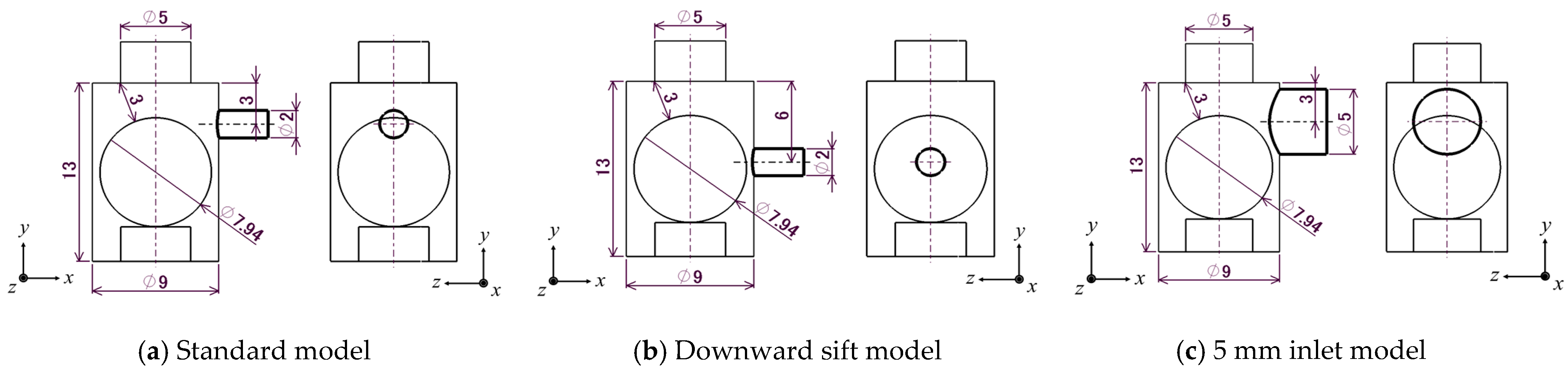
The four models used in this study are shown in Figure 3. In Figure 3a, the diameter of the inlet pipe is 2 mm, the diameter of the outlet pipe is 5 mm, the longitudinal inlet pipe position from the top of the housing to the center of the inlet pipe is 3 mm, the diameter of the housing is 9 mm, the height of the housing is 13 mm, and the diameter of the ball is 7.94 mm. Figure 3b shows the model in (a), with the inlet pipe position at 6 mm from the top. Figure 3c shows the inlet pipe of Model (a) with a diameter of 5 mm. The positive direction from the check ball to the inlet pipe is defined as the x-axis, the positive direction from the check ball to the outlet pipe is defined as the y-axis, and the axis perpendicular to both the x-axis and y-axis is defined as the z-axis. The shortest distance from the edge of the outlet pipe to the ball surface is defined as the initial lift (Lift; L) of 3 mm.
2.5. CAE Analysis Conditions
The turbulence model used in this study is a low-Re-type k–ε model that can accurately calculate the flow close to the object. The repulsion coefficient between the check ball and the enclosure was set to 0.2, and the constant time interval was set to 2.0 × 10⁻⁴ s. The gravity was considered to be 9.81 m/s2 in the negative direction of the y-axis. For the physical properties, S35C carbon steel was used for the check ball as the mechanical structure, and the hydraulic fluid was incompressible. Regarding the boundary conditions, a flow rate of 9.5 cc/s was specified at the inlet face, and the natural inflow-outflow condition was applied to the outlet face. The analytical conditions are listed in Table 1. To calculate the Reynolds number, the diameter of the inlet pipe was considered as a representative length. Although the Reynolds number was relatively small, swirling flow was generated in the confined area between the cylindrical housing and the spherical check ball, and the above-mentioned turbulence model was used to capture the separation phenomenon as the flow moved upward from the ball. The following two models were used to represent the state of motion of the complex elements of the check ball: (1) a six-degree-of-freedom model, wherein the check ball can rotate and translate; (2) a three-degree-of-freedom model, wherein the check ball can only translate. The kinematic viscosity of the hydraulic fluid was set to 7 mm2/s, which is the range of common hydraulic fluids, and 35.1 mm2/s, which is high viscosity; the flow rate was set to 9.5 cm3/s. The experiments were conducted under the calculation conditions listed in Table 1. However, for Model (c), with a diameter of 5 mm, the flow rate was increased by a factor of 2.5 to match the Reynolds number. Therefore, the flow velocity was reduced by a quarter.
3. CAE Analysis Results
3.1. Effect of Kinetic Viscosity of Hydraulic Fluid on Ball Behavior
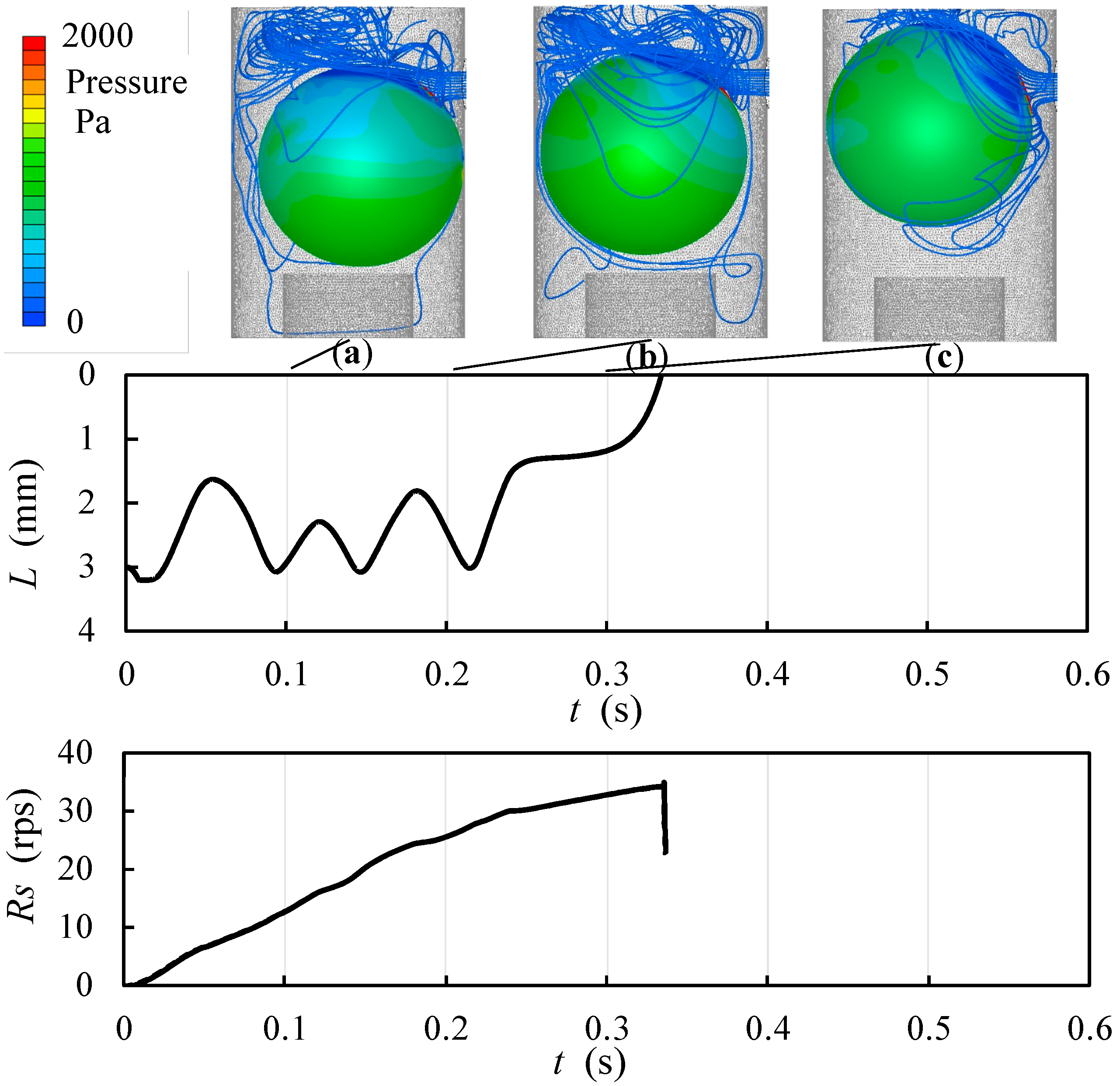
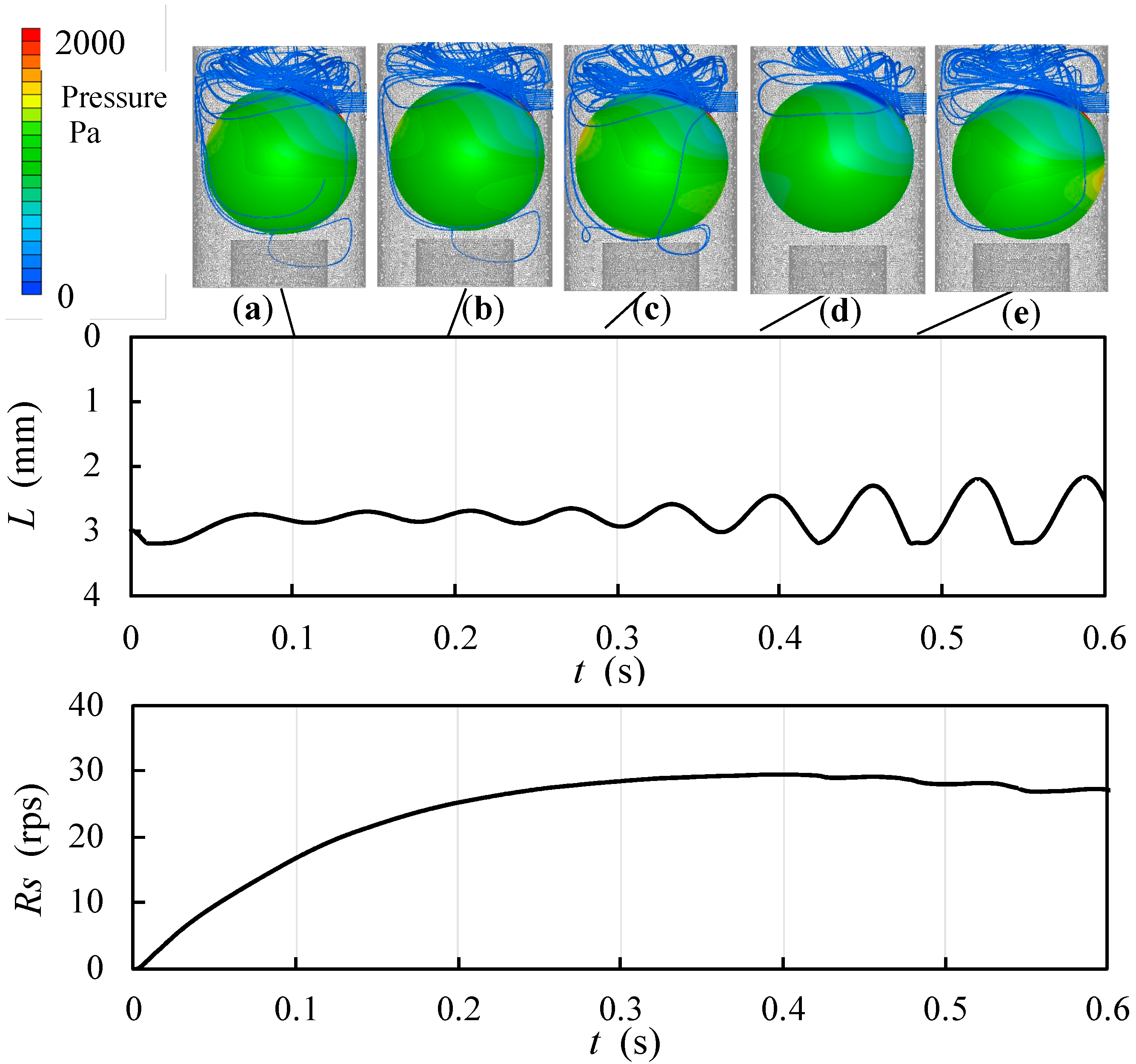
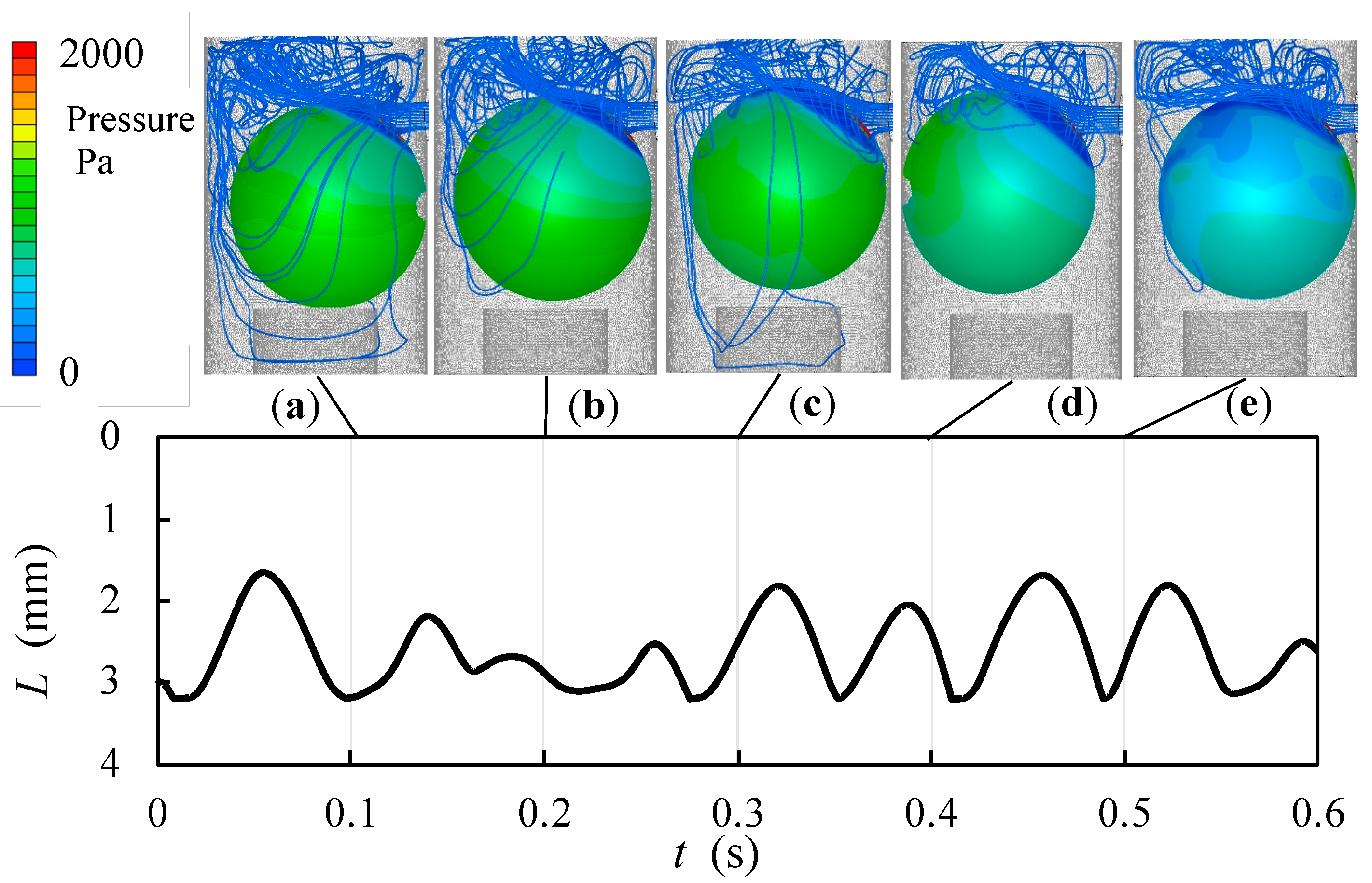
The CAE analysis results are presented below. Figure 4 shows the time variation of the lift, the rotation speed, and the CAE analysis results for the low-viscosity case. Here, t, L, and Rs represents time, the lift, and the rotational speed, respectively. Figure 5 shows the results for the high-viscosity case. Figure 4 and Figure 5 also show the ball surface pressure and flow lines at the respective times. Figure 4 shows that the time required for the check ball to rise to the surface was 0.34 s for the low-viscosity Model (a). The figure shows both the lift and the rotation speed obtained from the experiment [11]. It can be seen that the rotation speed and lift are consistent between the CAE analysis and the experiment. In the experiment, the ball position and the number of rotations were measured from the image analysis, so the measurement period was 0.1 s. However, as shown in Figure 5, the ball oscillated upward and downward and did not surface. In Figure 4, the ball moved upward and downward with the flow, and the rotation speed of the ball increased. Thus, it was found that the ball rose upward when the rotation speed of the ball was approximately 30 rps or more. The period of the upward and downward motion by the flow was approximately 0.05–0.08 s, and the amplitude was 1.5 mm. In the case shown in Figure 5, wherein the kinematic viscosity of the hydraulic fluid was high, the amplitude was similar and ranged from 0.06–0.08 s. The amplitude was as small as 0.2 mm. In the case of Figure 4, the amplitude began to increase when the rotation speed of the ball exceeded approximately 30 rps. However, in the case of high viscosity, the rotational speed of the ball did not exceed 30 rps but became constant, and the ball only oscillated upward and downward. In both cases, the ball rotated counterclockwise, as shown in Figure 4 and Figure 5, and the time required for the ball to reach a rotational speed of 30 rps was 0.3 s. In other words, the development of the circulating flow caused by the rotational motion of the check ball is considered to have increased the Magnus force acting on it.
Next, we performed an analysis with a limited number of degrees of freedom, which is a feature of the CAE simulation. In other words, the three degrees of freedom of rotation were fixed, and only translational motion was allowed. Figure 6 shows the time variation of the lift in the case of low viscosity. By comparing Figure 4 and Figure 6, it can be seen that the effect of rotation was small up to approximately 15 rps and until approximately 0.1 s, and the amount of lift of the ball was approximately the same. However, the effect of the Magnus force increased with the rotation speed, and the behavior changed. From the CAE analysis with restricted ball rotation, it was found that the ball oscillated upward and downward when it could not rotate. In other words, the Magnus force caused by the rotation of the ball plays a very important role in lifting the ball.
3.2. Effect of the Vertical Position of the Inlet Pipe on the Ball Behavior
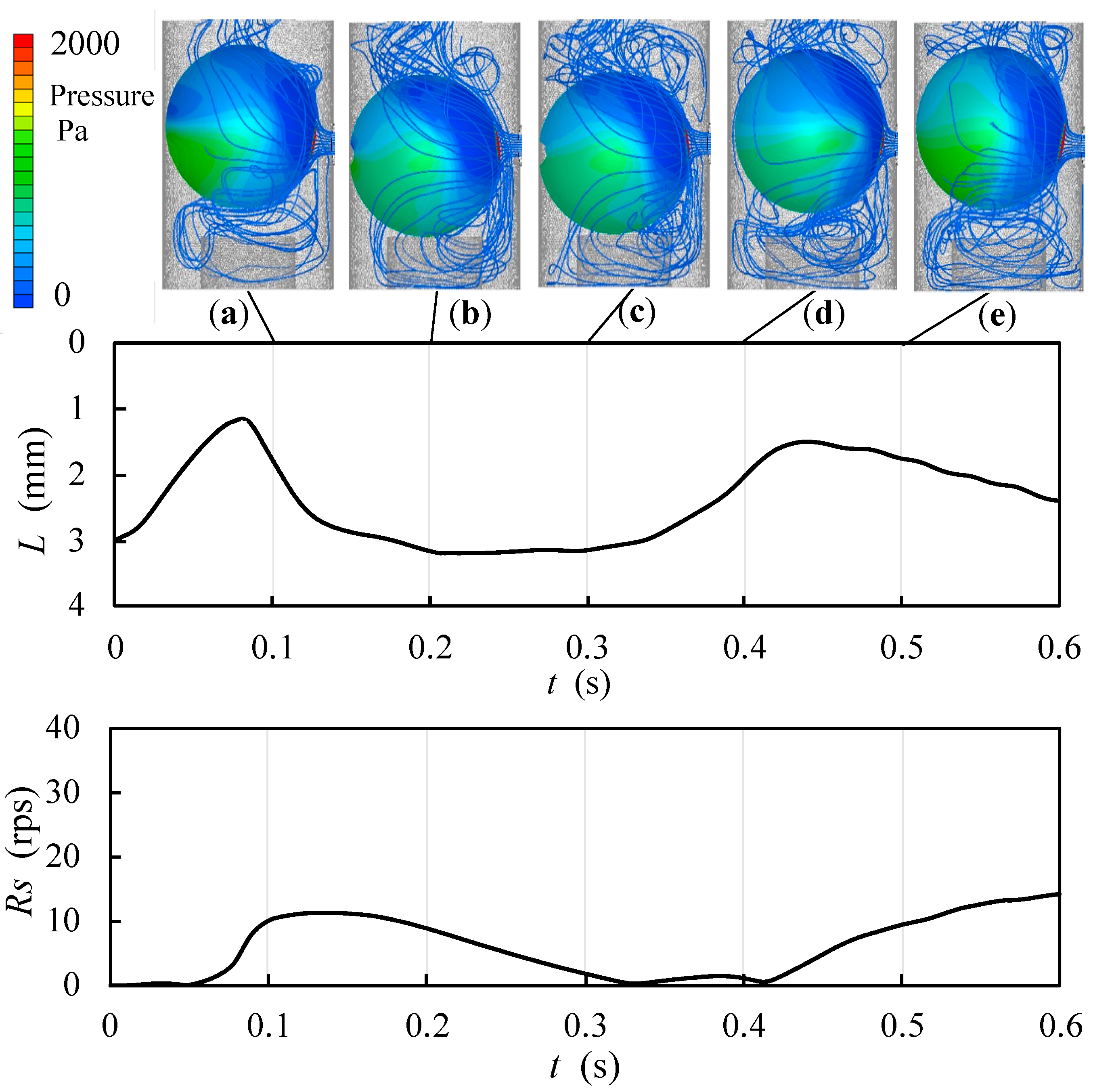
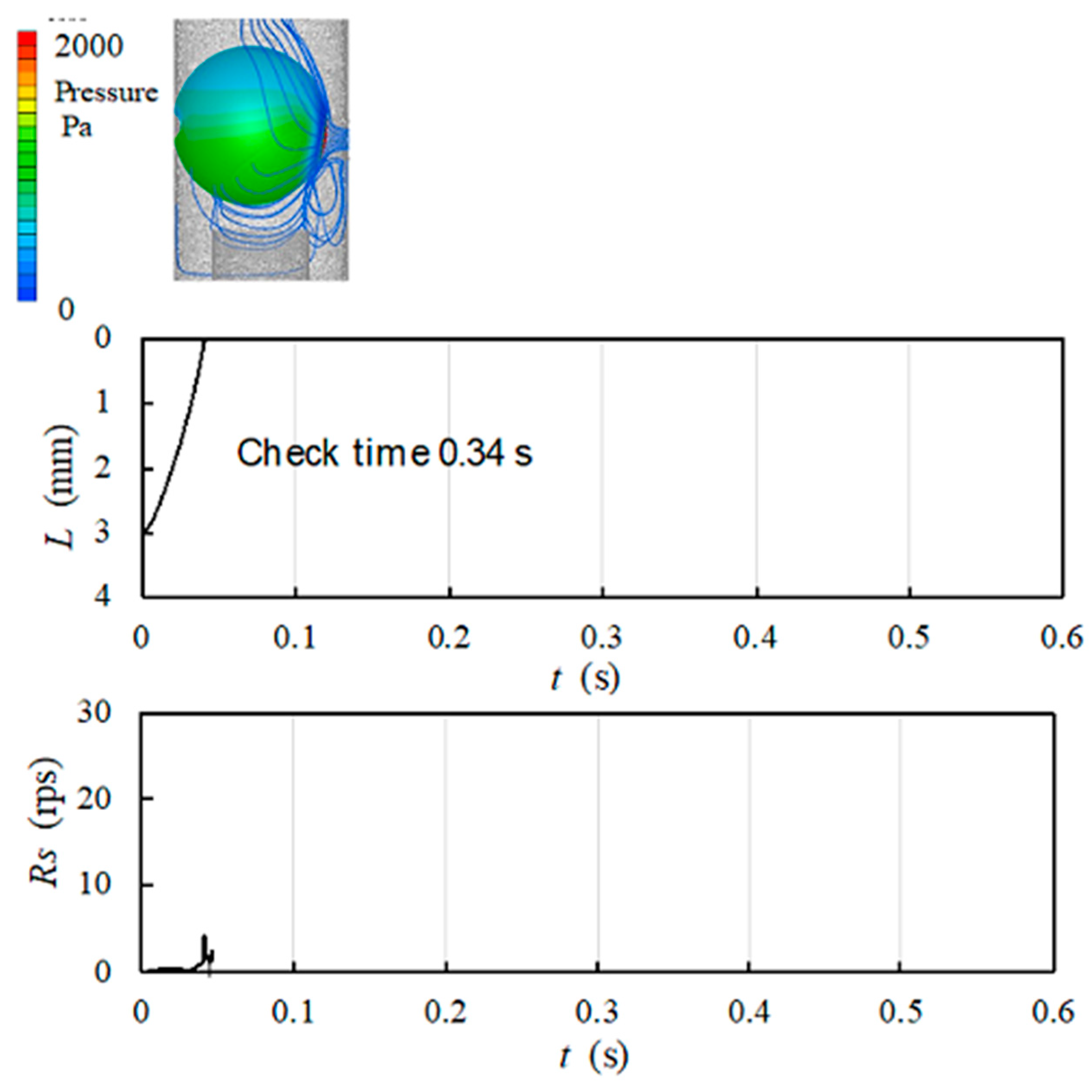
The time variations of the position and rotation speed of the ball in Model (b) are shown in Figure 7 and Figure 8, which show the low-viscosity case and high-viscosity case, respectively. In the low-viscosity case shown in Figure 7, the check ball did not rise to the surface, but was instead lifted to approximately 1 mm by 0.1 s. However, as the check ball rose, a strong jet hit the bottom of the ball causing it to rotate counterclockwise. This rotation generated a downward Magnus force, which increased the lift. As shown in Figure 3b, at the initial position, the inlet pipe was almost at the center of the ball. At approximately 0.08 s, when the lift was approximately 1 mm, the inflowing hydraulic fluid hit the bottom of the ball, causing it to rotate clockwise. At 0.2–0.3 s, the lift was 3 mm and the rotation speed was reduced because the inflowing oil jet hit the center of the ball. The pressure contour plot of the ball surface at 0.1 s indicates that the pressure difference between the left and the right side of the ball was large, and there was almost no pressure difference between the top and bottom. In the case of high viscosity shown in Figure 8, the mainstream was at the top of the ball, and the pressure at the top of the ball decreased owing to the flow velocity difference. Hence, the pressure difference between the top and bottom of the ball increased, and the ball rose rapidly. At this time, the ball hardly rotated, and the rotation effect was negligible.
Figure 9 shows the relationship between the lift and time for Model (b) with fixed degrees of freedom for rotation. Compared with the 6-DOF case shown in Figure 7, the lift was almost the same up to approximately 0.1 s without the effect of rotation. However, after 0.08 s, the lift increased owing to the effect of rotation and the downward Magnus force. In the analysis with fixed rotation, the pressure difference between the upper and lower parts of the ball almost disappeared after approximately 2 mm of lift, and the ball did not rise because the pressure difference mainly existed on the left and right sides of the ball. The figures show that the ball did not increase when the viscosity was low, but did increase when the viscosity was high. In the high-viscosity case, the same result was obtained for the 3-DOF case with fixed rotation. In other words, the rotational force on the ball was very small because the inlet was located at the center of the ball. The pressure distribution on the surface of the ball indicates that there existed a pressure difference between the left and right sides of the ball in the low-viscosity case, and the force on the ball acts from right to left in the figure.
The effect of the change in the vertical position of the inlet pipe on the behavior of the ball was evaluated by comparing the above-mentioned figures to Figure 4 and Figure 5.
In Model (a), the inlet pipe was located above the enclosure, and the fluid force acting downward was small; therefore, the jet hit the top of the ball and exerted a rotational force on the ball. Additionally, a velocity difference was produced above the ball and resulted in a pressure distribution that favored levitation. As shown in Figure 7, Figure 8, Figure 9 and Figure 10, in Model (b), the inlet pipe was at a lower position, which caused a velocity difference across the ball and resulted in lower pressure. Therefore, the fluid force was the main force. Because this fluid force increased with the viscosity, in the high-viscosity case, the ball rose in very short time. However, in the low-viscosity case, the fluid force was small and the downward Magnus force acted as the ball rotated counterclockwise, which made the increase even more difficult. However, when the rotation was fixed, the fluid force was not large, and the ball oscillated upward and downward to approximately 2 mm.
3.3. Effect of Inlet Diameter on Ball Rotation and Translational Motion
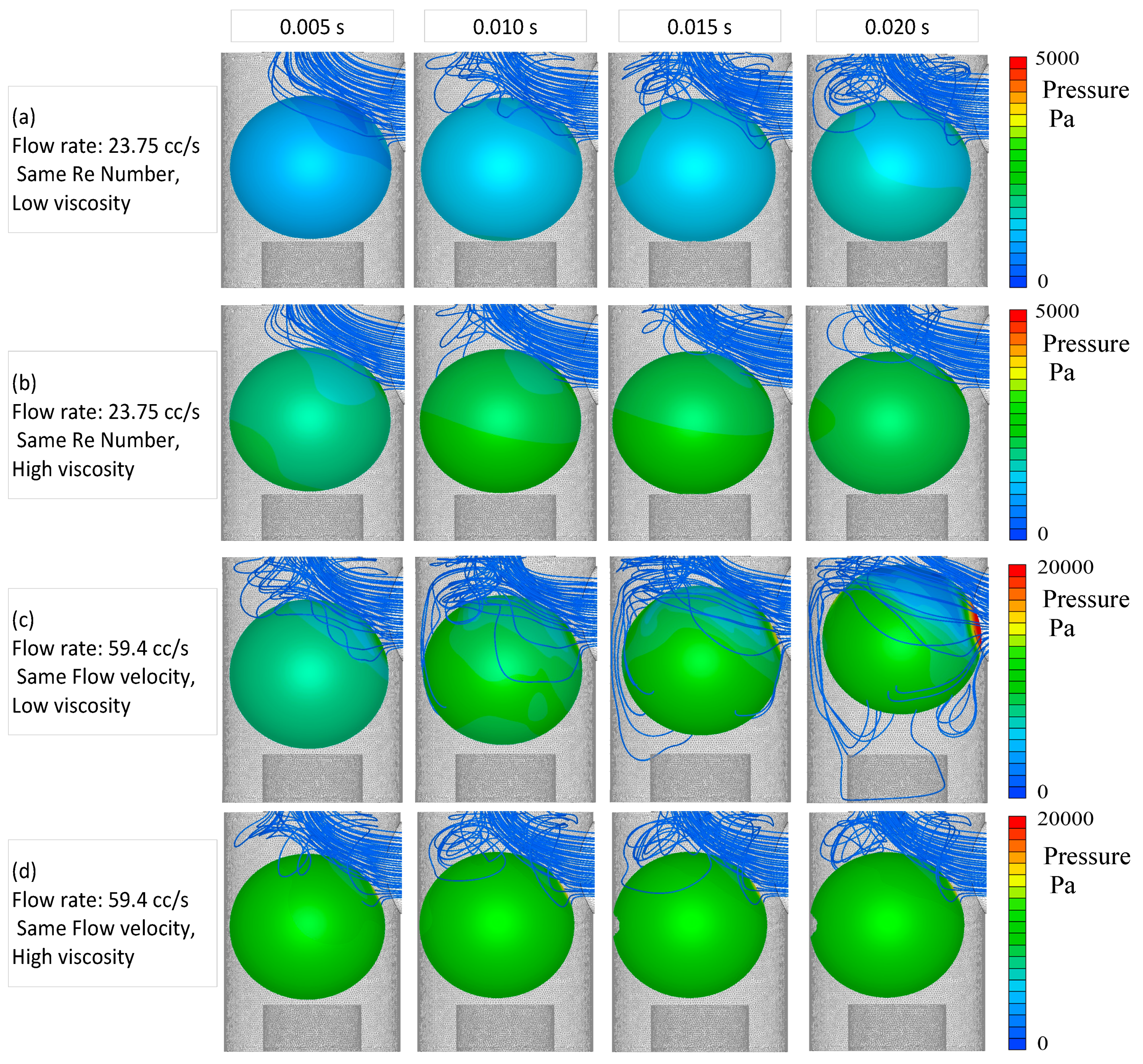
To clarify the relationship between the flow velocity and the rotational force of the ball, CAE analysis was also carried out for Model (c), wherein the inlet diameter was the same as the outlet diameter (5 mm). However, because the diameter of the inlet was increased by a factor of 2.5, the flow rate was increased by a factor of 2.5 to maintain the same Reynolds number. The results of the analysis revealed that, even with the same Reynolds number, the check balls did not rise to the surface in either the low- or the high-viscosity case, and the rotation of the balls was not observed. Next, the flow rate was increased by a factor of 2.5 × 2.5 to ensure that the velocity of the jet from the inlet pipe was the same. Under this condition, the ball floated in the low-viscosity case, but not in the high-viscosity case. Figure 10 shows the surface pressure distribution of the ball and the trace lines in these cases. In both cases, the ball surface pressure distribution was high at the upper right and low at the lower left. In the case of low viscosity, the flow was observed to move around the surface of the ball, and as the flow rate increased, the flow entered the lower part of the ball, causing the ball to float. However, in the case of high viscosity, there was almost no flow to the bottom of the ball and the ball did not float. When the inlet pipe was placed at the top and had larger thickness, the ball did not rotate in either case. In the case of Model (c), the ball increased only when the Reynolds number was the highest (2 × 10³). When the flow rate was maximum and the viscosity was low, the trajectory line indicates that the turbulence was high and the flow went around the bottom of the ball.
4. Discussion
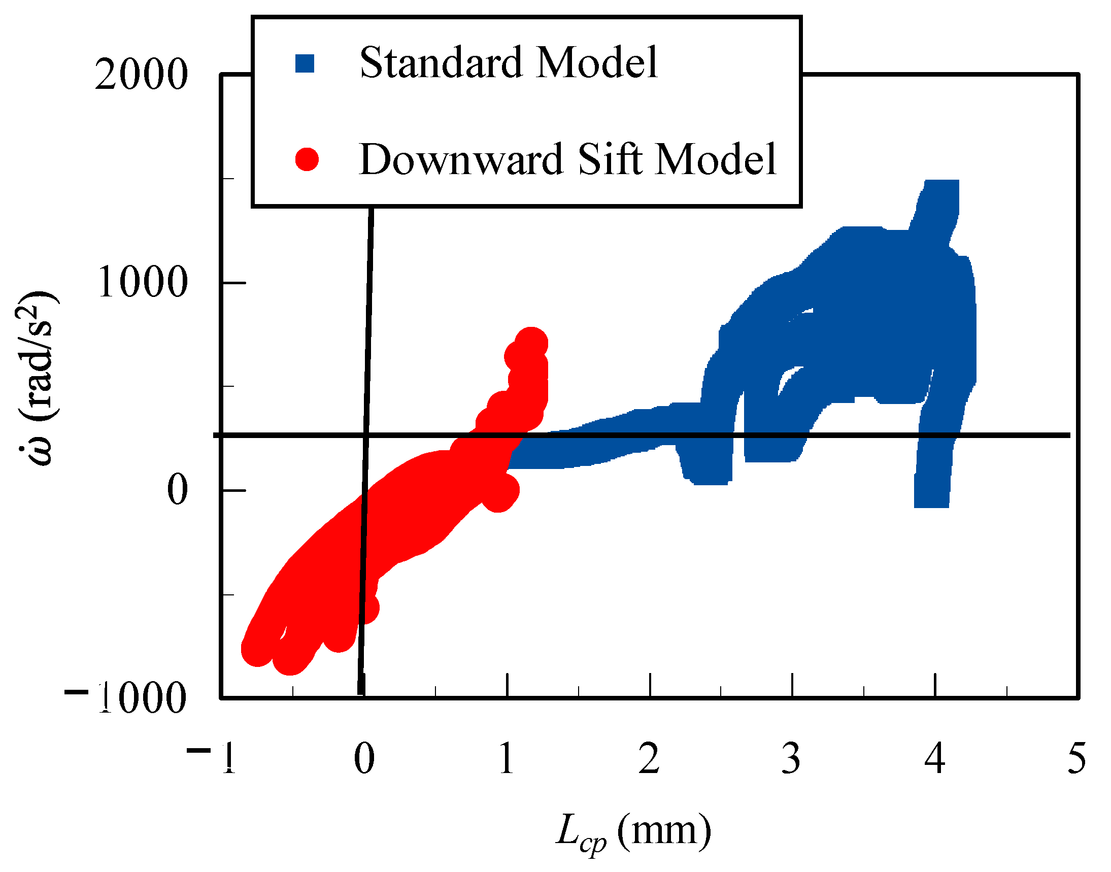
Based on the above-mentioned results, it is expected that the rotational speed and acceleration of the ball can be determined by the positional relationship between the inlet pipe and the ball. Therefore, we evaluated the rotational force of the ball caused by the oil jet from the inlet pipe. Figure 11 shows the relationship of the distance between the center of gravity of the ball and the center of the inlet pipe with the rotational angular acceleration. Here, Lcp and represents the distance between the center of gravity of the ball and the center of the inlet pipe with the rotational angular acceleration, respectively. The rotational acceleration on the vertical axis was calculated by differentiating the result for the number of rotations of the ball around the z-axis. The positive values on the x-axis indicate clockwise rotation, while the negative values indicate counterclockwise rotation. In the figure, blue indicates the standard model and red indicates the model with a downward shift. As can be seen, the positional relationship between the jet and the ball and the rotational acceleration are almost proportional. The main flow entered from the right side of the figure and moved upward, which indicates that the counterclockwise force acted even when the distance between the center of gravity of the ball and the inlet was zero. This figure suggests that the center of the inlet pipe should be placed at least 0.5 mm above the center of gravity of the ball to provide the clockwise rotation required to raise the ball.
5. Summary/Conclusions
The objective of this study was to realize a hydraulic ball valve that does not use springs. Experiments with many parameters, such as the oil viscosity, lift, diameter, and inlet position are costly, but there is a strong need to eliminate the spring owing to the problem of ball chattering, which causes the fracture of the spring. Hence, CAE analysis was carried out to measure the time variation of the ball position and rotational speed when the inflow position and viscosity of the hydraulic fluid changed. The flow in the piping was visualized, the effect of the Magnus force caused by the ball rotation on the ball levitation was clarified, and the interaction between the flow and the ball was elucidated. In the experiment, the check flow rate and rotation speed were measured by changing the inflow position of the hydraulic fluid, and the flow around the ball was visualized.
The results obtained by this study reveal that there was a difference in the effect of the jet flow on the rotational force of the ball between the high-viscosity case and low-viscosity case. The rotational force of the ball was determined by the positional relationship between the ball and the inlet pipe, and a large Magnus force was generated when the rotation speed increased. This Magnus force caused the ball to rise. If the positional relationship between the ball and the inlet pipe is such that the ball rotates counterclockwise, the ball is not expected to rise, even if a large flow rate is applied. Owing to the interaction of various parameters, such as the relative position of the ball and the position of the inlet, which determines the strength of the fluid jet, the above-mentioned parameters must be considered.
The main conclusions drawn from this study are as follows:
- (1)
- CAE analysis using a polymerized grid was carried out to observe the flow around the check ball, surface pressure, and rotation speed;
- (2)
- The Magnus force caused by the ball rotation was evaluated by carrying out CAE analysis with fixed rotation and only translation being allowed;
- (3)
- When the inlet pipe was at the top, the ball did not rise when there was no rotation or when the viscosity was high;
- (4)
- As the rotation speed of the check ball increased, circulating flow developed, the Magnus force increased, and the ball rose faster;
- (5)
- If the position of the inflow pipe shifted downward, there was almost no rotation; if the viscosity was low, the ball did not rise;
- (6)
- The Magnus force acting on the check ball changed depending on the direction of the rotational motion of the check ball;
- (7)
- The Magnus force caused the check ball to rotate faster.
Because various parameters that determine the strength of the fluid jet, such as the relative position of the ball and the position and diameter of the inlet, interact with each other, the authors plan to deepen their understanding of this phenomenon and make quantitative observations in future work.
Funding
This research received no external funding.
Acknowledgments
Shinji KAJIWARA is acknowledged for his contribution to the completion of this article.
Conflicts of Interest
The author declares no conflict of interest.
References
- Tsukiji, T.; Suzuki, Y. Numerical simulation of an unsteady axisymmetric flow in a poppet valve using the vortex method. ESAIM 1996, 1, 415–427. [Google Scholar] [CrossRef] [Green Version]
- Hong, F.G.X.; Huayong, Y.; Tsukiji, T. Numerical and experimental investigation of cavitating flow in oil hydraulic ball valve. In Proceedings of the Fifth JFPS International Symposium on Fluid Power NARA, Nara, Japan, 12–15 November 2002; Volume 2, pp. 923–928. [Google Scholar]
- Hayase, T.; Humpherey, J.A.C.; Greif, R. A consistently formulated QUICK scheme for fast and stable convergence using finite-volume iterative calculation procedures. J. Comput. Phys. 2013, 1, 108–118. [Google Scholar]
- Grossschmidt, G.; Harf, M. Part 1: Fundamentals, COCO-SIM object-oriented multi-pole modelling and simulation environment for fluid power systems. Int. J. Fluid Power 2009, 10, 91–100. [Google Scholar]
- Sen, S.; Mittal, S. Free vibration of a square cylinder at low Reynolds numbers. J. Fluids Struct. 2011, 27, 875–884. [Google Scholar] [CrossRef]
- Yonezawaa, K.; Ogawa, R.; Ogi, K.; Takino, T.; Tsujimoto, Y.; Endo, T.; Tezuka, K.; Morita, R.; Inada, F. Flow-induced vibration of a steam control valve. J. Fluids Struct. 2012, 35, 76–88. [Google Scholar] [CrossRef]
- Lee, H.; Lee, T.; Chang, Y. Numerical simulation of flow-induced bi-directional oscillations. J. Fluids Struct. 2013, 37, 220–231. [Google Scholar] [CrossRef]
- Zhao, M. Numerical investigation of two-degree-of-freedom vortex-induced vibration of a circular cylinder in oscillatory flow. J. Fluids Struct. 2013, 39, 41–59. [Google Scholar] [CrossRef]
- Goncalves, R.T.; Rosetti, G.F.; Franzini, G.R.; Meneghini, J.R.; Fujarra, A.L.C. Two-degree-of-freedom vortex-induced vibration of circular cylinders with very low aspect ratio and small mass ratio. J. Fluids Struct. 2013, 39, 237–257. [Google Scholar] [CrossRef]
- Kajiwara, S. Experimental observations of the fluid flow within the L-shaped check valve. Int. J. Fluid Power 2013, 14, 17–23. [Google Scholar] [CrossRef]
- Kajiwara, S. Effect of the check ball and inlet position on hydraulic L-shaped check ball behavior. J. Fluids Struct. 2014, 48, 497–506. [Google Scholar] [CrossRef]
- White, B.R.; Schulz, J.C. Magnus effect in saltation. J. Fluid Mech. 1977, 13, 497–512. [Google Scholar] [CrossRef]
- Abe, K.; Kondoh, T.; Nagano, Y. A new turbulence model for predicting fluid flow and heat transfer in separating and reattaching flows—I. Flow field calculations. Int. J. Heat Mass Transf. 1994, 37, 139–151. [Google Scholar] [CrossRef]
- Hirt, C.W.; Amsden, A.A.; Cook, J.L. An arbitrary Lagrangian-Eulerian computing method for all flow speeds. J. Comput. Phys. 1974, 14, 227–253. [Google Scholar] [CrossRef]
Figure 1.
Schematic View of Dumper Cylinder.

Figure 2.
Mesh arrangement around the check ball and housing.

Figure 3.
CAE models. Model (a) Standard model; Model (b) Downward sift model; Model (c) 5mm inlet model.
Figure 3.
CAE models. Model (a) Standard model; Model (b) Downward sift model; Model (c) 5mm inlet model.

Figure 4.
Time variation of lift and rotation speed in low-viscosity case of Model (a): Streamlines and ball surface pressure distribution (a) 0.1 s, (b) 0.2 s, (c) 0.3 s.
Figure 4.
Time variation of lift and rotation speed in low-viscosity case of Model (a): Streamlines and ball surface pressure distribution (a) 0.1 s, (b) 0.2 s, (c) 0.3 s.

Figure 5.
Time variation of lift and rotation speed in high-viscosity case of Model (a): Streamlines and ball surface pressure distribution (a) 0.1 s, (b) 0.2 s, (c) 0.3 s, (d) 0.4 s, (e) 0.5 s.
Figure 5.
Time variation of lift and rotation speed in high-viscosity case of Model (a): Streamlines and ball surface pressure distribution (a) 0.1 s, (b) 0.2 s, (c) 0.3 s, (d) 0.4 s, (e) 0.5 s.

Figure 6.
Time variation of lift in low-viscosity case with three degrees of freedom of Model (a): Streamlines and ball surface pressure distribution (a) 0.1 s, (b) 0.2 s, (c) 0.3 s, (d) 0.4 s, (e) 0.5 s.
Figure 6.
Time variation of lift in low-viscosity case with three degrees of freedom of Model (a): Streamlines and ball surface pressure distribution (a) 0.1 s, (b) 0.2 s, (c) 0.3 s, (d) 0.4 s, (e) 0.5 s.

Figure 7.
Time variation of lift and rotation speed in low-viscosity case of Model (b): Streamlines and ball surface pressure distribution (a) 0.1 s, (b) 0.2 s, (c) 0.3 s, (d) 0.4 s (e) 0.5 s.
Figure 7.
Time variation of lift and rotation speed in low-viscosity case of Model (b): Streamlines and ball surface pressure distribution (a) 0.1 s, (b) 0.2 s, (c) 0.3 s, (d) 0.4 s (e) 0.5 s.

Figure 8.
Time variation of lift and rotation speed in high-viscosity case of Model (b); Streamlines and ball surface pressure distribution 0.02 s.
Figure 8.
Time variation of lift and rotation speed in high-viscosity case of Model (b); Streamlines and ball surface pressure distribution 0.02 s.

Figure 9.
Time variation of lift for low-viscosity case with three degrees of freedom of Model (b); Streamlines and ball surface pressure distribution (a) 0.1 s, (b) 0.2 s, (c) 0.3 s, (d) 0.4 s (e) 0.5 s.
Figure 9.
Time variation of lift for low-viscosity case with three degrees of freedom of Model (b); Streamlines and ball surface pressure distribution (a) 0.1 s, (b) 0.2 s, (c) 0.3 s, (d) 0.4 s (e) 0.5 s.

Figure 10.
Time variation of lift for low-viscosity case with three degrees of freedom of Model (b): (a) Flow rate: 23.75 cc/s, Same Re Number, Low viscosity; (b) Flow rate: 23.75 cc/s, Same Re Number, High viscosity; (c) Flow rate: 59.4 cc/s, Same Flow velocity, Low viscosity; (d) Flow rate: 59.4 cc/s, Same Flow velocity, Low viscosity.

Figure 11.
Relationship of distance between center of gravity of ball and center of inlet pipe and rotational angular acceleration.
Figure 11.
Relationship of distance between center of gravity of ball and center of inlet pipe and rotational angular acceleration.


Table 1.
Physical properties and numerical conditions.
| Variable | Value | |||||
|---|---|---|---|---|---|---|
| Inlet Diameter (mm) | 2 | 5 | 5 | |||
| Inlet Flow Velocity (m/s) | 3.02 | 1.21 | 3.02 | |||
| Fluid Density, r (kg/m3) | 868.6 | 868.6 | 868.6 | |||
| Inlet Volume Flow Rate (m3/s) | 9.5 × 10⁻⁶ | 23.75 × 10⁻⁶ | 59.4 × 10⁻⁶ | |||
| Kinematic Viscosity, n (mm2/s) | 7 | 35.1 | 7 | 35.1 | 7 | 35.1 |
| Reynolds Number, Re | 8.57 × 10² | 1.71 × 10² | 8.57 × 10² | 1.71 × 10² | 21.4 × 10² | 4.28 × 10² |
Publisher’s Note: MDPI stays neutral with regard to jurisdictional claims in published maps and institutional affiliations. |
© 2021 by the author. Licensee MDPI, Basel, Switzerland. This article is an open access article distributed under the terms and conditions of the Creative Commons Attribution (CC BY) license (https://creativecommons.org/licenses/by/4.0/).
Share and Cite
MDPI and ACS Style
Kajiwara, S. Evaluation of Magnus Force on Check Ball Behavior in a Hydraulic L Shaped Pipe. Fluids 2021, 6, 191. https://0-doi-org.brum.beds.ac.uk/10.3390/fluids6050191
AMA Style
Kajiwara S. Evaluation of Magnus Force on Check Ball Behavior in a Hydraulic L Shaped Pipe. Fluids. 2021; 6(5):191. https://0-doi-org.brum.beds.ac.uk/10.3390/fluids6050191
Chicago/Turabian StyleKajiwara, Shinji. 2021. "Evaluation of Magnus Force on Check Ball Behavior in a Hydraulic L Shaped Pipe" Fluids 6, no. 5: 191. https://0-doi-org.brum.beds.ac.uk/10.3390/fluids6050191