
Towards Reconstruction of Complex Flow Fields Using Unit Flows

1
Mechanical Engineering Department, Texas A&M University, College Station, TX 77840, USA
2
Nuclear Engineering Department, Texas A&M University, College Station, TX 77843, USA
3
Ocean Engineering Department, Texas A&M University, College Station, TX 77843, USA
*
Author to whom correspondence should be addressed.
Fluids 2021, 6(7), 255; https://0-doi-org.brum.beds.ac.uk/10.3390/fluids6070255
Submission received: 8 May 2021
/
Revised: 25 June 2021
/
Accepted: 5 July 2021
/
Published: 13 July 2021
(This article belongs to the Special Issue Scientific Computing in Fluids)
Abstract
:Many complex turbulent flows in nature and engineering can be qualitatively regarded as being constituted of multiple simpler unit flows. The objective of this work is to characterize the coherent structures in such complex flows as a combination of constituent unitary flow structures for the purpose of reduced-order representation. While turbulence is clearly a non-linear phenomenon, we aim to establish the degree to which the optimally weighted superposition of unitary flow structures can represent the complex flow structures. The rationale for investigating such superposition stems from the fact that the large-scale coherent structures are generated by underlying flow instabilities that may be reasonably described using linear analysis. Clearly, the degree of validity of superposition will depend on the flow under consideration. In this work, we take the first step toward establishing a procedure for investigating superposition. Experimental data of single and triple tandem jets in crossflow are used to demonstrate the procedure. A composite triple tandem jet flow field is generated from optimal superposition of single jet data and compared against ‘true’ triple jet data. Direct comparisons between the true and composite fields are made for spatial, temporal, and kinetic energy content. The large-scale features (obtained from proper orthogonal decomposition or POD) of true and composite tandem jet wakes exhibit nearly 70% agreement in terms of modal eigenvector correlation. Corresponding eigenvalues reveal that the kinetic energy of the flow is also emulated with only a slight overprediction. Temporal frequency features are also examined in an effort to completely characterize POD modes. The proposed method serves as a foundation for more rigorous and robust dimensional reduction in complex flows based on unit flow modes.
1. Introduction and Motivation
Fluid mechanics research has traditionally employed canonical flows as a means of determining the dominant mechanisms of naturally occurring flow phenomena, relying exclusively on scientific discovery from first principles. Regarding more complex flows found in nature and engineering, high-fidelity parameterization of geometric, kinematic, and dynamic quantities of interest have proven costly for iterative optimization, for both experiments and simulations alike [1]. There exists then a significant area of possible contributions for data-driven methods that seeks not to replace, but to compliment traditional means of understanding, modeling, optimization, and control of complex fluid flows.
Decomposition methods such as proper orthogonal serve as the plausible candidate in more robust reconstruction methods of complex flows from their unit bases. These techniques are a fundamental cornerstone of data-driven engineering and no stranger to fluid mechanics and turbulence research. Such methods seek to exploit the evolution of coherent structures or patterns in large data sets, i.e., fluid flows, to construct low-order models of the complex fluid motions. Decompositions represent the data as a linear combination of basis elements, called modes, that separate the spatial and temporal structures via their shared energy contributions [2].
The current investigation seeks to examine a different avenue for rapid reconstruction of complex flow fields and reduced (but still useful) level of fidelity. It is evident from visual inspection that complex flows are composed of multiple distinct physical features and phenomena. For example, any complex wake of a bluff body is comprised of von Kárman shedding [3,4], Kelvin–Helmholtz instability [5], and vortex pairing/merging [6]. The individual features and phenomena can be isolated and examined in canonical unit flows with relative ease [7,8,9] both in laboratory experiments and numerical simulations. Significant advances in high spatio-temporal resolution experimental imaging and high-fidelity numerical simulations have generated a wealth of two- and three-dimensional velocity field data on such flow phenomena for visualization and exploration. These velocity fields represent the primary means of understanding the underlying vortex dynamics and turbulent stresses of such flow topologies from both the human’s [7] and computer’s [10] interpretation of the associated physics. It is reasonable then to postulate that the large-scale turbulent structures of complex flows are similar to those in unit flows and differ only in component magnitudes, shapes, and/or frequency. These notions prompt an overwhelming query for applied fluid mechanics: can complex fluid topologies be reconstructed from suitably combining canonical unit flow features?
The current investigation provides a foundation for potential reconstruction methods by first examining a linearly weighted superposition of the primitive variables, i.e., velocity fields, directly. While the current motive is concerned with high spatio-temporal fidelity data sets found in fluid experiments and simulations, apparent extensions for more general scalar fields and imaging applications will be evident. By setting a non-biased global criterion, features are extracted from the primitive data, without the need for a priori knowledge or expertise. This is especially attractive for complex flows. Many of these flows may consist of repetitive geometries containing several turbulence generating devices. By appointing a unit cell basis, these devices are typically identified as simple canonical flow types, or unit flows, such as homogenous grid turbulence, jets, wakes, and mixing layers which have been studied extensively in classical turbulence theory [11,12,13]. Replication or reconstruction of complex flows from appropriate unit flows is challenging due to the non-linear interactions, where kinematic and dynamic exchanges promote secondary features and effects, not present in the underlying unit flow(s). On the other hand, the linear potential flow theory has enjoyed qualified success in many aerodynamic and hydrodynamic flows for computing basic forces and flow patterns. Superposition of potential theory solutions of different unit flow fields to capture basic features of complex flows often serves as the first step in many multi-fidelity CFD (computational fluid dynamics) approaches [14]. Indeed, the so-called Panel Method is still used in the fields of aerodynamics and hydrodynamics for yielding rapid-turnaround calculations for multi-disciplinary optimization.
The objective of the present work is to examine the use of spatial superposition of linearly weighted unit flows as a means of reconstructing a complex flow by optimizing certain objective functions. The methodology applies elements of image editing, linear algebra, and optimization to an arbitrary high-fidelity physics-based data set. To re-iterate, the method is generalizable and little a priori information or expertise about the physics, i.e., mechanics, itself is needed. Experimental data of unit and complex flows are used to verify the degree of validity and utility of the proposed superposition approach. The investigation that follows provides sufficient evidence that the composite weighted unit flows share sufficient spatial and temporal information with that of their corresponding ‘true’ measured complex data sets, linked via their eigenvalues as assessed via each data set’s proper orthogonal decomposition (POD).
Section 2 provides a brief review of the POD matrix factorization used to generalize the eigen decomposition of rectangular matrices found in high-fidelity experimental and numerical fluid flow data. The review is provided in anticipation of evaluating the superposition approach for such data sets, formally introduced in Section 3. The methodology provides a flexible framework to overlay/stitch and linearly weight sub-domains of the unit flow(s), whose summation provides a composite imitation of the ‘true’ measured or simulated complex flow. The composite and ‘true’ data sets can then be assessed effectively via their corresponding POD constituents. There exist several possible extensions for frequency-based or hybrid decompositions. However, no effort is provided here. In Section 4, the methodology is applied to time-resolved particle image velocimetry (TR-PIV) data of a single and three tandem round jets in a crossflow, where the latter exhibits complicated secondary interactions as a result of shielding provided by each jet with its neighbor(s) [15]. The cross-sectional plane measurements of the single and tandem jet arrays share the same general physical features and phenomena and constitute the unit and complex flows, respectively. It is found that low-order dimensional approximations of the complex fluid flow’s spatial, energetic, and temporal behaviors are possible with the use of weighted sub-domains of the associated unit flow type. Current optimal weightings are based on limited velocity field information, i.e., the aforementioned sub-domains of the flows, from the optical measurement field of view and current limitations are acknowledged.
The article concludes with a discussion surrounding perhaps the most important consequence of this work. The proposed weighted superposition method and the well-known POD are both inherently linear representations of the primitive unit flow data. This implies that the POD eigenvectors themselves may be used, in place of the velocity data, in a similar linearly weighted superposition procedure over large ranges of Reynolds or Mach numbers, where the coherent structures are known to differ only in their size, shape, and frequency of observation. The authors envision a more robust reconstruction strategy employing these cataloged mode shapes, with more refined weightings provided by advanced machine learning (ML) algorithms, to greatly reduce the number of experiments or simulations needed to effectively reproduce complex fluid flows of interest.
2. Dimensionality Reduction via POD
Originating from the Karhunen–Loève theorem [16], POD is used in several fields of science and may also be referred to as principal component analysis, Hotelling analysis, empirical component analysis, quasi-harmonic modes, empirical eigenfunction decomposition, etc. [9]. POD was originally introduced to the fluid mechanics community by Lumley [17], who sought to relate the spatial structures of the modes with the corresponding coherent structures in turbulent flows. One of the most attractive features of the POD is that its modes provide an optimal (in a least squares sense) orthogonal basis of the stochastic process. The POD’s emphasis on spatial formations and energy optimality makes it fundamentally valuable to the current effort: it provides a coordinate transform and reduction to simplify the dynamics and low-order flow physics [18,19]. The technique has become a staple of a wider class of dimensionality reduction techniques, whose major objective is to extract key features and dominant patterns that yield reduced coordinates thereby adequately describing the input data more compactly and efficiently [9].
It is important to distinguish the objectives of the POD for data-driven applications from that of reduced-order modeling (ROM). Extensive efforts in model reduction have employed Galerkin projection of the Navier–Stokes equations onto an orthogonal basis of POD modes [20]. Unsteady behaviors in the flow field may yield certain low-energy states that exhibit large influence on the dynamics, but do not significantly contribute to the low-order POD modes. While the modes may be optimal for the input data set, they are frequently not optimal for the Galerkin projection [21]. Such methods are closely tied to the governing equations, constrained by first principles of empirical understanding. In general, ROM methods are considered intrusive and require human expertise for model development. The quintessential difference for data-driven methodologies, in the context of fluid physics, is the incorporation of ML algorithms for identification and modeling, which rely only on partial a priori knowledge of the governing equations, constraints, and symmetries [22]. This does not imply that decomposition methods, or the larger array of potential ML algorithms available, may be applied naively. Such methods are blind to the basic physics and its inherent constraints and dynamics [10]. It is well known that the POD performs well for statistically stationary periodic flow types, but may perform poorly for non-normal systems experiencing significant transients or unsteady behaviors [23]. The current work discusses application of the POD in terms of high-fidelity experimental or numerical fluid flow data, though the technique and methodology that follows is consistent with the broader range of imaging and pattern recognition with excellent references provided by [24,25].
The current investigation utilizes the singular value decomposition (SVD) method, briefly reviewed here using the convention provided by references [9,26]. The SVD is a general decomposition technique for rectangular matrices [27,28], and the POD is a decomposition formalism. The SVD represents only one possible method to solve the POD and is accompanied by the classical method [29] and the method of snapshots [30,31,32], where the latter can be found throughout the fluid mechanics and turbulence literature. The SVD is ideal for the proposed work in that it is generalizable, easily implemented, and computationally inexpensive. The data set, , here pertaining to velocity components , is first organized into columns according to Equation (1).
The reshaped data set consists of column vectors of the fluid velocity, where is the number of discrete vector points in a given frame, and is the number of snapshots, in the data set. It is beneficial to compute the row-wise mean according to:
with corresponding mean matrix
and subtract this column vector from the data matrix . The non-mean-subtracted and mean-subtracted data sets are understood as the instantaneous and fluctuating field data, respectively. It is common knowledge in the fluid mechanics community that either rendition produces the same hierarchical modes, with the exception of the instantaneous field’s first mode representing the time-averaged field and its second mode being nearly identical to that of the fluctuating field’s first mode. The time-averaged modal representation is valuable for the current objective and as such, the instantaneous quantities are preferred here.
The SVD of data matrix is formulated according to Equation (4).
where , and , and where for TR-PIV measurements and is the transpose. Matrix consists of real, non-negative entries along its diagonal and zeros everywhere else. Given that , matrix has a maximum of non-zero elements along its diagonal. It is useful then to employ the economy SVD to exactly represent according to Equation (5).
where implies the economy-sized decomposition of the matrix (zeros removed), is the orthogonal compliment, and hence, the columns of and span vector spaces that are complimentary and orthogonal. Matrices and are unitary matrices consisting of orthonormal columns referred to as the left singular vectors and right singular vectors of , respectively. It should be noted that in the instance where contains , the economy SVD will instead contain a maximum of non-zero elements along its diagonal. The columns of are more formally known as the eigenvectors. The diagonal elements of are the singular values, denoted by , , … and are ordered from largest to smallest. For completeness, it should be stated that the singular values held in and are identical to the eigenvectors of and , respectively. Thus, the singular values are directly related to the eigenvalues, , via the relation [9]. The data matrix , i.e., a velocity component field is effectively decomposed into three parts by the POD, separating the physical characteristics into spatially orthogonal modes and corresponding temporal contributions, via their hierarchically ranked eigenvalues.
Mode truncation is the primary concern in reconstructing a low-order approximation of the original data matrix . Major factors include the desired rank of the system, noise magnitude, and the distribution of singular values, or inherently, the eigenvalues of the system [26]. Many authors opt for a heuristic approach to determine the rank that provides a pre-allocated amount of variance (energy) of the original data, typically 80%, 90% or 99%. The current work favors the optimal hard thresholding criteria of Gavish and Donoho [33]. The authors view truncation as a hard threshold of the singular values, where values larger than are kept, and the remaining values are removed. This method assumes that the input data matrix consists of low rank structure contaminated Gaussian white noise according to Equation (6).
where the magnitude of the noise is denoted by and the entries of are assumed independent and identically distributed Gaussian random variables with zero mean and unit variance. In the case of turbulent flow data, the noise magnitude is generally unknown, in which case the optimal hard threshold estimates the noise magnitude and scales the distribution of singular values according to the median singular value, . This implies that there is no closed form solution and is approximated numerically according to Equation (7).
where , the parameter , and is the solution to Equation (8).
3. Linearly Weighted Superposition for Complex Flow Reconstruction
The linearly weighted superposition is first presented in the example using the cross-sectional wake formations of the single and tandem jets in a crossflow. The section concludes with a formal summary and generalized strategy for reconstruction of complex data sets form their unit basis/bases.
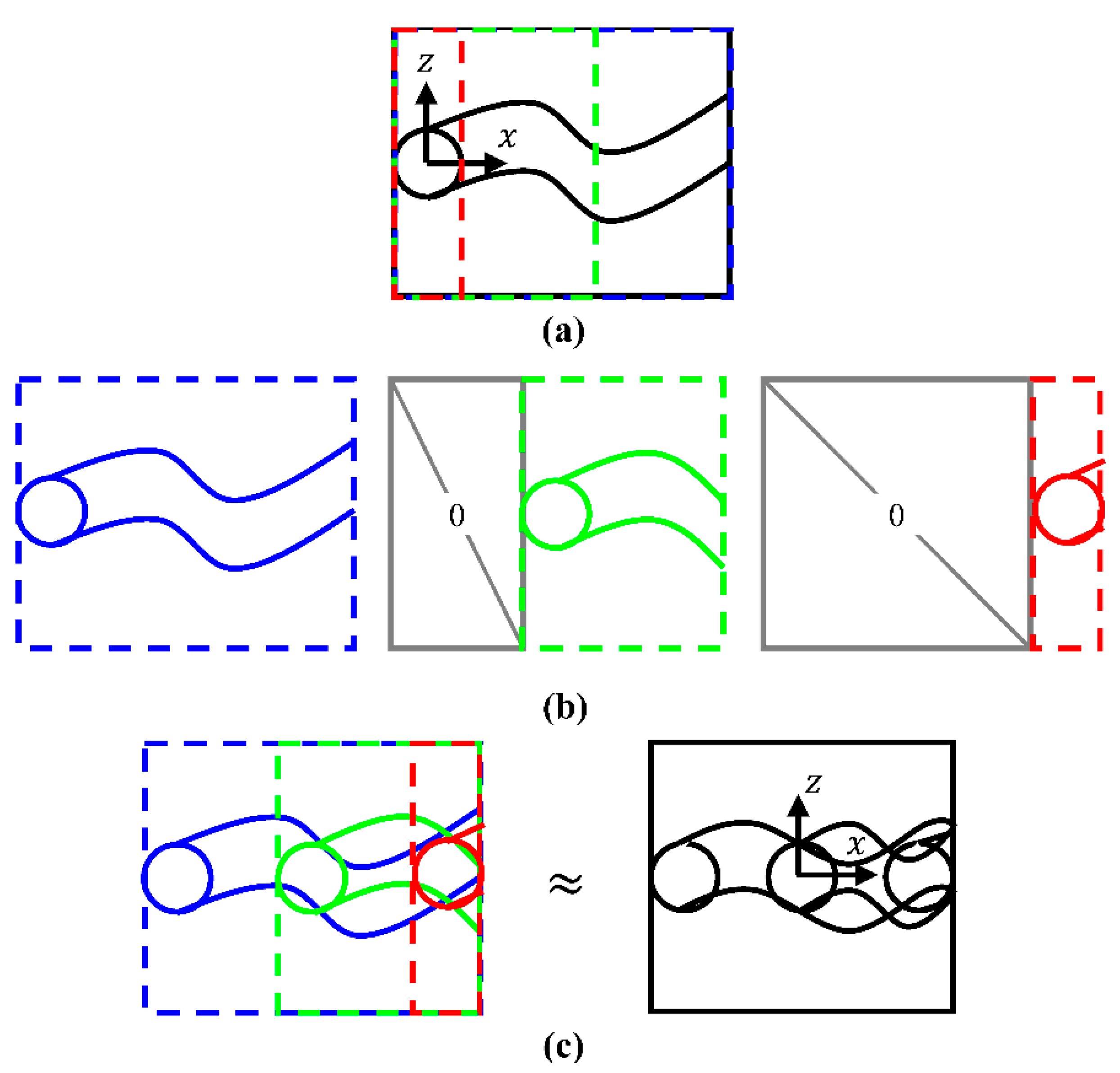
As alluded to at the end of Section 2, there is a general pattern or similarity shared by each jets’ penetration, wake formation, and periodic flapping that has the potential to be modeled using only data available from the single jet in crossflow, the unit flow in this instance. The methodology is visualized in Figure 1 which for the current investigation applies to the streamwise and spanwise velocity components, ) and , respectively. As seen in Figure 1a, the single jet measurement data (black) is duplicated and cropped into three sub-domains (blue, green, and red). From Figure 1b, each sub-domain’s cropped indices are carefully chosen to directly overlay with the Cartesian coordinate positions of the first (blue), second (green), and third (red), based on the available measurement field of view, with supplemental zeros (gray) imposed on non-existent upstream conditions as seen in Figure 1b. The sizing of each null matrix ensures that each of the sub-domains consists of an identical number of rows and columns, or and , respectively. In reference to Figure 1c, there exists an independent constant scalar weighting for each of the three velocity field sub-domains, that when overlaid and summed together, i.e., a weighted average (overlaid blue, green, and red), can provided a reasonable approximation of the complex fluid flow data (black), to be further assessed by low-order dimensional reduction.
The current weighting procedure employs a simple quadratic programming scheme. The objective function to be solved is displayed in Equation (9).
Here, each column of x is a sub-domain matrix stored as a column vector, and since there are three sub-domains (), is an 3 matrix and is the ‘true’ measured or numerical data set, i.e., an 1 array. The term is also an 1 array and corresponds to each sub-domain’s ‘weight’ to be determined. Recognizing that and , Equation (9) readily simplifies to:
the third term of which is constant with respect to 𝑤 and is therefore discarded during minimization. From Equation (10), the quadratic objective term, , and linear objective term, , are appointed according to Equations (11) and (12), respectively.
We then define linearity equality constraints and = 1 and a lower bound of zero to ensure non-negative weightings. Finally, the problem is fully specified according to Equation (13).
which is solved using >>w=quadprog(H,f,[],[],Aeq,beq,lb) in MATLAB to provide the optimized weights for each sub-domain [34]. As alluded to prior, the weighted averaged comprises the composite data set,
which is compared to the ‘true’ data set, , via their corresponding PODs.
In review, the methodology is formally proposed according to Algorithm 1 provided below.
| Algorithm 1. Given a two-dimensional, high spatio-temporal complex flow topology produced by experiment or numerical simulation and here prescribed as the ‘true’ data set , proceed as follows. |
|
| * “Placement” may refer to stitching sub-domains side by side if spaced sufficiently far apart or overlapping if secondary mixing interactions are plausible. ** Typical matrix transformations: stretching, rotation, reflection as discussed in any reputable linear algebra textbook. |
The principal goal of this work is to establish the extent of validity of linear superposition and quantify the effects of non-linearity. The superposition methodology proposed here is applicable any complex flow field data that consists of repetitive canonical flow(s) as its basis(es), e.g., jets, bluff bodies. The input data set is inherently a function of spatial and temporal coordinates, with sufficient resolution of each (i.e., a global representation), and does not rely on underlying knowledge of the governing equations. The weighting functions of superposition are expected to be flow dependent. Guidelines for determining the weighting functions for unseen flows will be developed in future works.
Th extension of the unit flow superposition methodology for flows with multi-scale coherent structures (e.g., wall-bounded turbulence) requires further development. These flows consist of several dominant eddies, spaced sufficiently far apart such that they act independently of one another [35]. Global representations are not effective in such instances, since the associated coherent structures are essentially unrelated. Such flows are better suited for a hierarchical approach using the minimum flow concept [36]. Reconstruction of these flows entails superposition of multiple modes of different frequencies and horizontal spatial wavenumbers [37]. Such multiscale reconstruction will be attempted in future works.
In summary, Algorithm 1, Steps 1–2 describe the general unit basis of a larger series of patterned features. Step 3 employs intuitive image alterations and matrix transformations to effectively replicate the pattern from its fundamental repeating feature(s). Steps 4–7 provide the basis for weighted averages of each sub-domain via a generalized optimization strategy employing quadratic programming. The composite and “true” data sets are then compared via an appropriate decomposition as described in Steps 8–9. This methodology provides the fundamental framework for complex flow reconstruction via a linearly weighted superposition of the unit flow basis(es). The approach is now assessed for the unit and complex fluid problem at hand (Figure 1) and followed by a discussion of possible future avenues of enhancement.
4. Results: TR-PIV Data of Tandem Jets in a Crossflow
4.1. Description of Data Sets
The experimental data sets were collected using TR-PIV on a tandem array of three jets in a crossflow. A series of single jet experiments are provided at identical testing conditions to the tandem jets, serving as the unit flow basis as discussed previously in Section 3. Several authors have investigated the single jet in crossflow using POD and have identified several important coherent structures that occur as a result of unsteady boundary layer interactions, pressure gradients, turbulence, and vortex formations, and how these features develop as the jet momentum overcomes that of the crossflow [38,39,40,41,42]. Universal scaling laws have proven to be challenging and the addition of more than one jet only seeks to further complicate this objective, particularly in the range of low jet to crossflow velocity ratios (2). These flows are characterized by several important vortical formations including hairpin, horseshoe, shear layer, and wake vortices, as well as counter rotating vortex pairs [43] that each affect the statistically dominant flow features at different velocity ratios.
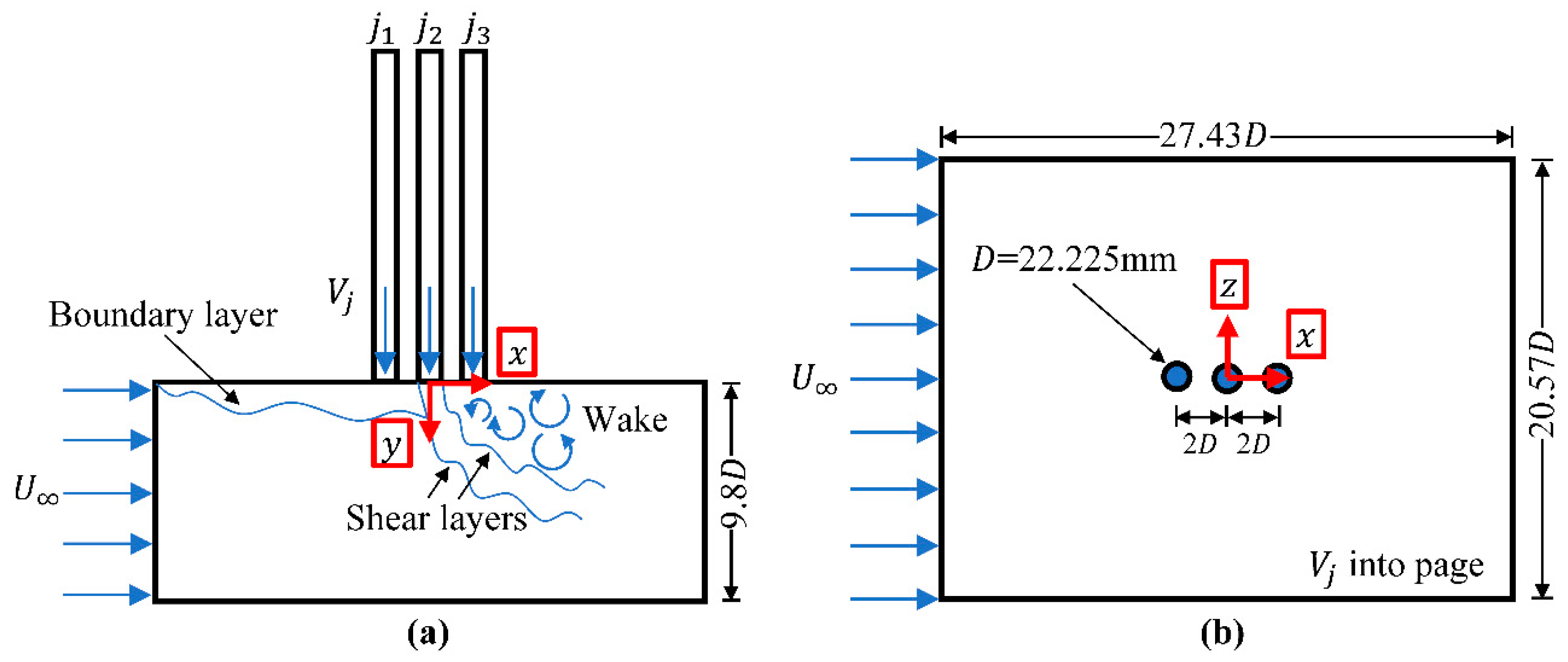
Full details regarding the experimental arrangement have been outlined previously [15,44] with pertinent details reviewed here. The experiment consists of a low speed wind tunnel test section with three round jets in a tandem formation issuing vertically downward from the ceiling of the test section as outlined in Figure 2. The tunnel inlet consists of a top-hat, low turbulence inlet profile and each of the three jets exhibit nearly identical flow rates and turbulent Reynolds numbers at their exits into the test section. The same conditions are confirmed for the single jet formation, utilizing only the middle jet with the upstream and downstream jets sealed flush. The single jet results form the unit flow basis for the more complex tandem jet array at identical testing conditions, which include three distinct jet to crossflow velocity ratios, = 0.9, 1.25, and 1.7. The inner diameter of each jet is = 22.225 mm with a center-to-center spacing of 2. The test section dimensions consist of 27.43, 9.8, and 20.57 in the , , and directions, respectively. The crossflow velocity and Reynolds number are 9.52 m/s and 1.82 105, respectively, which is held constant for all velocity ratios considered.
Both the crossflow and jets are seeded sequentially using a TSI Six Jet Atomizer (TSI Incorporated, Shoreview, MN, USA) with Dioctyl Sebacate tracer particles. Illumination is provided by a Photonics DM30-527-DH laser (Photonics Industries, Ronkonkoma, NY, USA) with a thickness of ~1 mm. Two Phantom Miro M120 CMOS cameras (Vision Research Inc., Wayne, NJ, USA) are mounted in a stereoscopic configuration and each is outfitted with a LaVision Scheimpflug Mount, Nikon AF NIKKOR 50 mm f/1.8D lens, and LaVision Inc. 527 nm bandpass filter (LaVision Inc., Ypsilanti, MI, USA). A high-quality silvered mirror is rigidly mounted at a 45° angle underneath the test section to provide optical access to the test section in the plane (Figure 2b).
The field of view is 207.2 mm 175.9 mm in the and directions, respectively, and is located at = 1. The laser and cameras are synchronized to provide 2600 image pairs at 1 kHz. The separation time is set to 116, 75, and 38 for = 0.9, 1.25, and 1.7, respectively, providing particle displacements of approximately 4–6 pixels in each image pair. Vector field generation is accomplished with LaVision DaVis 8.4.0 software. Pre-processing employs a Butterworth high pass filter with local 7 frame length to limit background noise. Vector processing utilizes the stereo cross-correlation algorithm with initial two passes using a 64 × 64 pixel window with 1:1 square weighting and 75% overlap and four final passes using a 32 × 32 pixel window with an adaptive PIV grid with 75% overlap. Vector generation produces 120 102 spatial grid points from the measurement field of view, constituting each instantaneous velocity field. Post-processing incorporates a ‘strongly remove and iteratively replace’ median filter, which removes vectors if the difference to the average is greater than 2 × root mean square (RMS) of its neighbors and re-inserts the vector if the difference to the average is less than 3 × RMS of its neighbors. As a final step, vector interpolation fills any holes in the instantaneous velocity field produced by the initial post-processing filter. This interpolation computes the average of all neighboring vectors surrounding the missing point, with a minimum of two neighbors for computation.
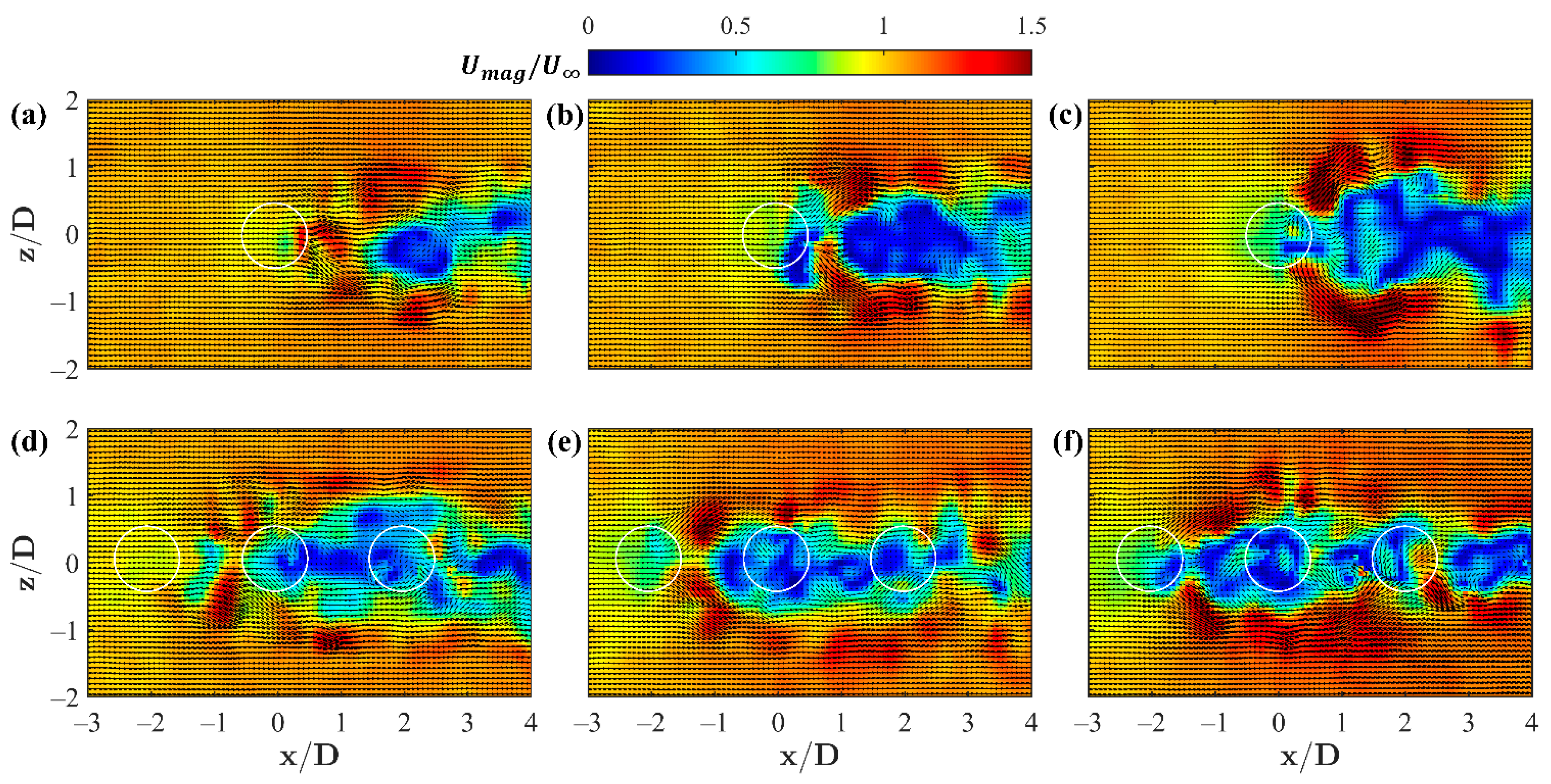
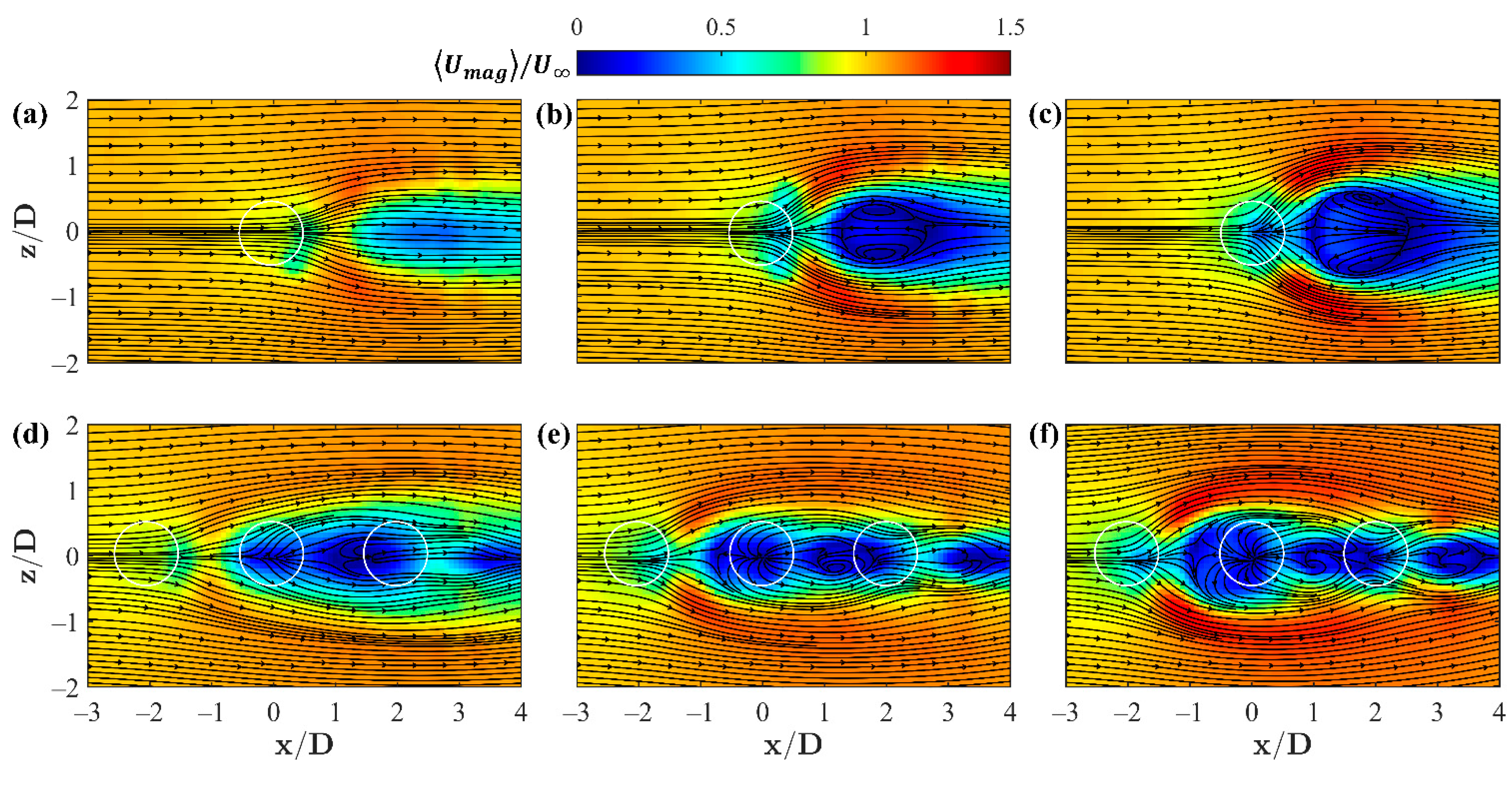
Instantaneous and time-averaged velocity magnitude profiles of the plane at = 1 have been observed previously in [15,44] and are reproduced here in Figure 3 and Figure 4. The single jet profiles in Figure 3a–c appear amorphous, as a result of the aggregation of several mechanisms induced by the two perpendicular flow streams and boundary layer interactions with the wall leading up to the jet. These effects include entrainment and mixing with the freestream, unsteady velocity fluctuations from turbulence, and the rotation induced in the flow as a result of these interactions. Several features drive the flow patterns found in this plane including periodic flapping of each jet’s wake, the outer shear layer interface with the uniform free stream, and recirculation zones as a result of the jet momentum, here into the plane, which acts to stall the perpendicular crossflow. The tandem jet configuration further complicates these interactions as the flow driving mechanisms become less clear, exhibiting more localized features as a result of the spatial proximity of each jet.
These features allow additional leverage in augmenting the data matrix for each velocity component investigated. As suggested by [45] in their flow past a cylinder example, each data matrix is augmented with a secondary set of snapshots, identical to the measurement data in , but flipped across the symmetric axis and corresponding sign change, according to Equation (15).
The method is mathematically sound and still entirely a function of the observed physics; used as a means of enforcing symmetry in the data set and strengthening signal correlation as a result of doubling the number of snapshots, This augmentation is applied to both and , after Equation (3) and before Equation (4). While having clear benefit for the current data set, this and similar augmentations require a basic understanding of the flow phenomenon and physical features before use and should thus be applied at the user’s discretion.
4.2. Optimal Weightings Based on Discrete Parameterization
As initially illustrated in Figure 1, the single jet wake is extracted, copied, and overlaid to imitate each of the three tandem jets (jets 1, 2, and 3). It should be noted that the field of view limits the available overlap for each segment to the range −2.54 2.48 and −2.04 2.04. From the initial investigation [15], the majority of this region encompasses the interaction between the first leading jet and the encapsulated middle jet. The optimal weightings for each segment’s corresponding velocity components and velocity ratios tested are provided in Table 1. As discussed in [15], the leading jet in the tandem array exhibits similar behaviors to that of the single jet and exhibits a shielding effect on its downstream neighboring jets. This notion is reflected here with the optimal weightings for jet 1 being substantially higher than jets 2 or 3. Given the limited experimental field of view, the weightings for jet 3 are minimal. It is believed that a substantially larger field of view would provide additional non-zero weightings for jet 3, as its influence becomes more apparent further downstream. With increasing velocity ratios and corresponding shielding, the downstream tandem jets penetrate further into the crossflow. This produces an interesting tradeoff, as the jet 1 and weightings appear inversely and directly proportional to , respectively. The opposite functional dependencies are found for the jet 2 weightings. The optimal weightings are now assessed via their composite data sets’ energy content (eigenvalues), spatial modes (eigenvectors), and temporal distributions.
4.3. Energy Spectra and Cumulative Energy Distributions
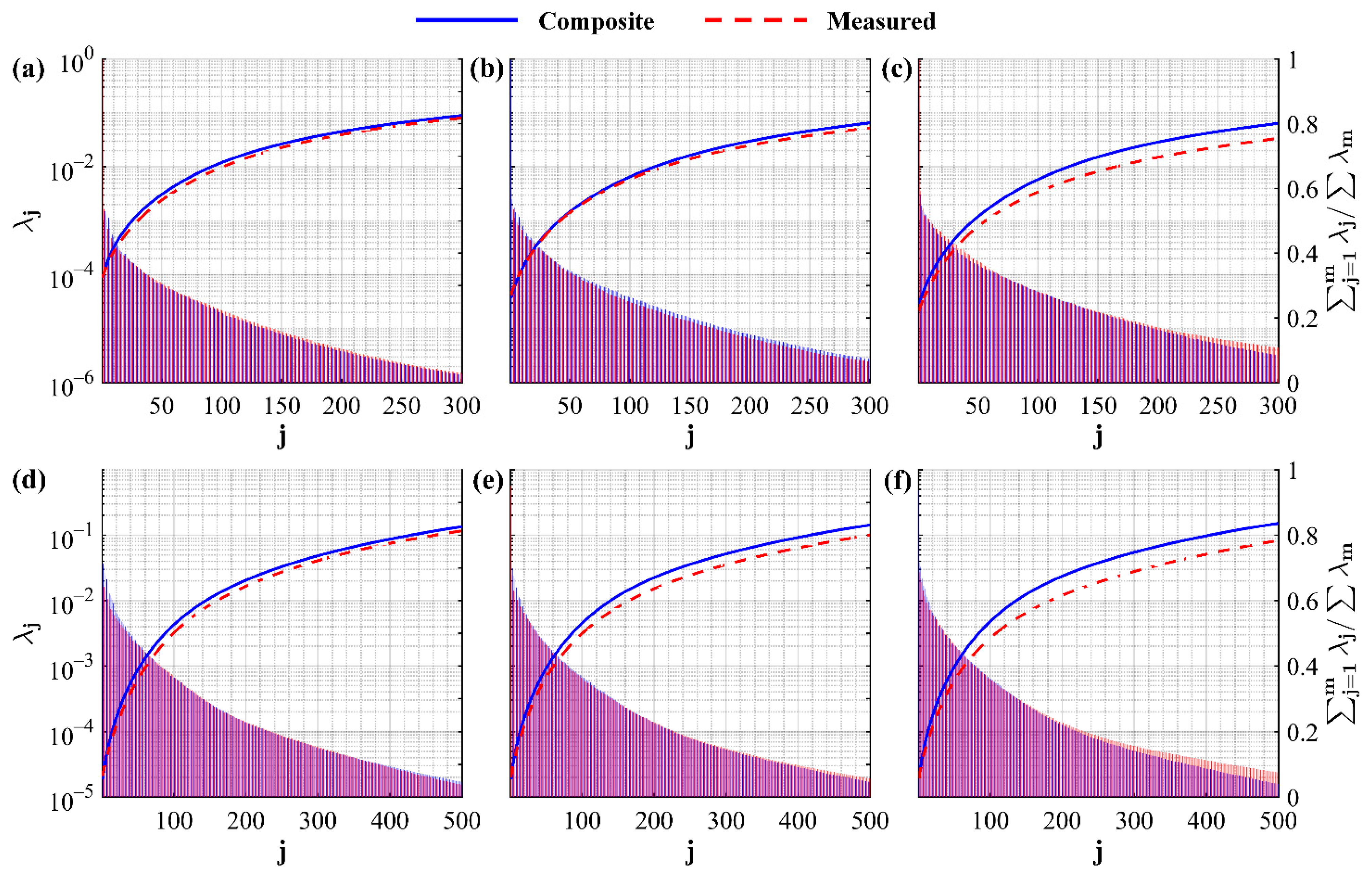
The energy spectra and cumulative energy for the composite and ‘true’ data sets are presented in Figure 5 for the dominant low-order modes, here representing approximately 80% of the kinetic energy of their corresponding velocity components. The composites promote eigenvalues that are remarkably similar to the true measured tandem jet data, across all three velocity ratios and both components of velocity. This is reaffirmed by the cumulative energy for each velocity ratio as a function of the increasing number of modes. Physically, this implies that the kinetic energy content of the tandem jet array is captured by the composite unit flows in both the streamwise and spanwise velocity formation of the jet wakes with a slight overprediction on behalf of the composites. In general, these trends follow nearly identical curves, implying that with possible further refinement of the data sets and/or weightings, a higher precision optimal composite may indeed overlap with the ‘true’ kinetic energy distribution. The current motive is merely to assess this procedure, via the constituents of the POD, to determine whether more robust numerical schemes are a likely avenue of success in determining improved optimal weightings via unit flows of more repetitive flow geometries.
Results of the optimal hard truncation for each data set are presented in Table 2. In general, the number of truncated modes, , for the measured and composite data sets provide similar quantities, with the composite truncations requiring slightly less modes for each velocity ratio. The maximum difference in between the composite and measured truncations is 1.2% for the = 0.9 velocity components. This difference is found to be a function of increasing velocity ratio, with a maximum difference of 15.7% found for the = 1.7. The singular value thresholds, , for the composite streamwise velocity component yield fairly similar trends, namely a low percent difference at the lowest velocity ratio (8.0%) which increases significantly at the highest velocity ratio (22.5%). The spanwise component’s cutoffs are more severely affected by the weighting procedure and differ from their measured comparisons. As discussed in Section 2, the optimal cutoff values are inherently based on the noise magnitude found in their corresponding data sets. The composites, however, must also consider the effect of segmenting and weighting the data. The authors have previously applied POD to the original single jet in crossflow data sets [15,44] and found the corresponding values to be nearly identical to that of the tandem jet, thereby confirming that the major culprit here is the segmentation and/or weighting. These cutoff values, however, do not take away from the success of the composite in replicating the eigenvalue magnitudes, cumulative energy distributions, and potential compression of the measured data set as displayed previously in Figure 5 and here in Table 2.
4.4. Eigenvectors
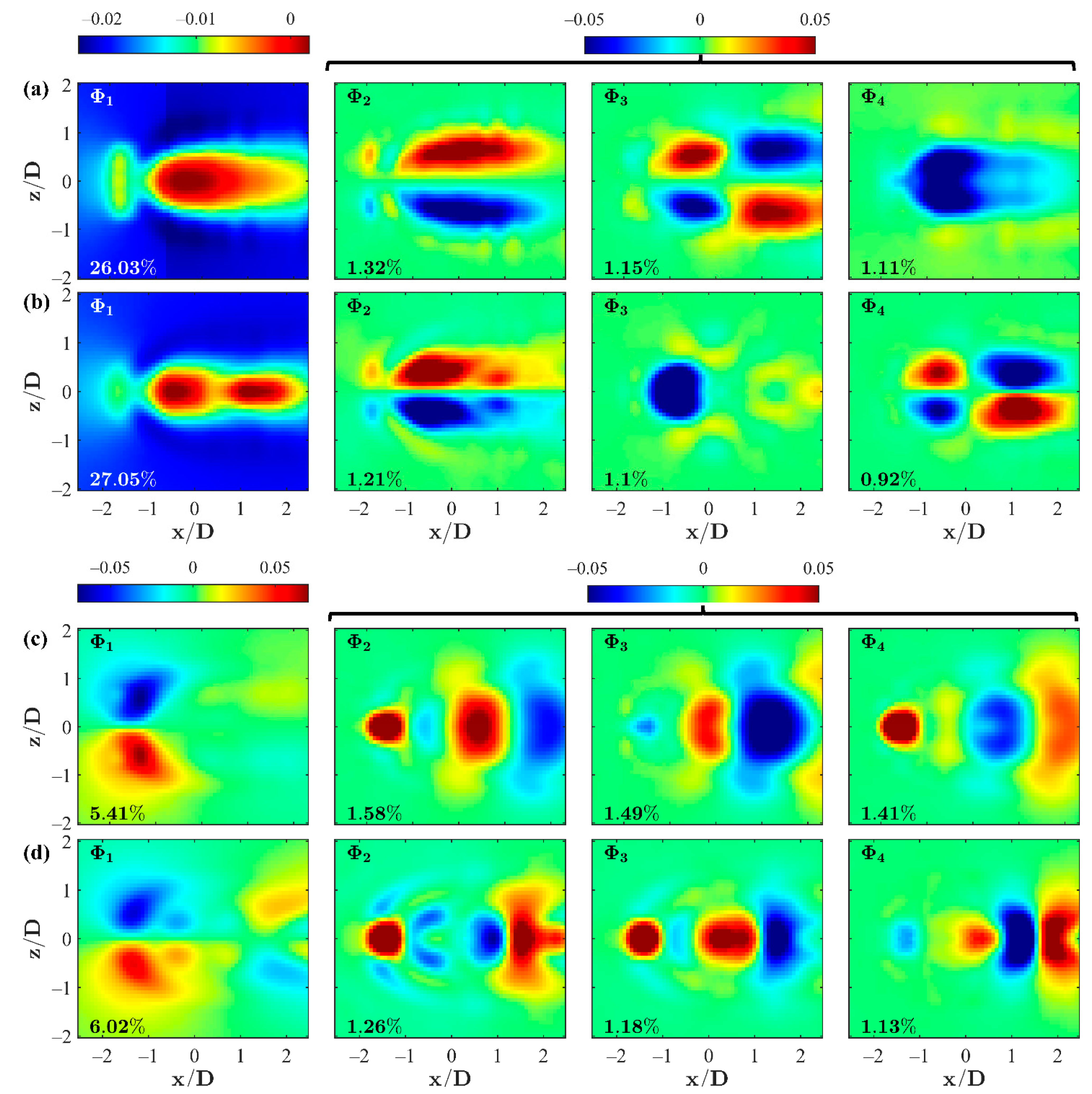
Low-order POD modes for the composite and measured data sets are provided in Figure 6, using the = 1.25 case as an example. It should be noted that the first mode and all modes greater than one are constrained by respective uniform color scalings for direct comparison. Given the preconditioning of the velocity fields (non-mean subtracted, i.e., instantaneous quantities) the first modes are statistically similar to the time-averaged velocity fields as seen in Figure 6a,c for the and components, respectively. The composite segments are slightly visible for the component’s , but do not extend visibly past the first mode. In general, clear similarities and discrepancies can be observed between the composite and measured modes. The comparison in Figure 6a,b shows that the coherent structures present in and are similar in both shape and magnitude. Perhaps more interesting is that the composite and agree quite well with the measured and , respectively. This implies that the same general coherent structures exist in the composite and measured data sets, with slightly different hierarchical rankings. The comparison in Figure 6c,d shows several relatively large and smaller-scale shapes. The composite data sets tend to capture the large-scale features and proximities, as expected. Regarding the smaller-scale structures, the composites exhibit weaker correlation strength, visibly understood as the faint, secondary shapes in Figure 6c compared to those present in Figure 6d. For a given test case and each velocity component, the first mode of the composite and measured data sets contain the majority of the kinetic energy, as expected, and offer nearly identical percentages of relative energy. For each mode thereafter, the relative kinetic energies for the composite and measured data sets are also in excellent agreement, with the component values performing slightly better than the component. These comparisons reflect the ability of the composite data and corresponding decompositions to accurately depict flow structures promoted by shear and localized eddies in the wake of the tandem jets as evident by the measured tandem jet data.
The eigenvector correlation, , is determined according to the dot product of the eigenvectors from the composite and measured data sets as seen in Equation (16).
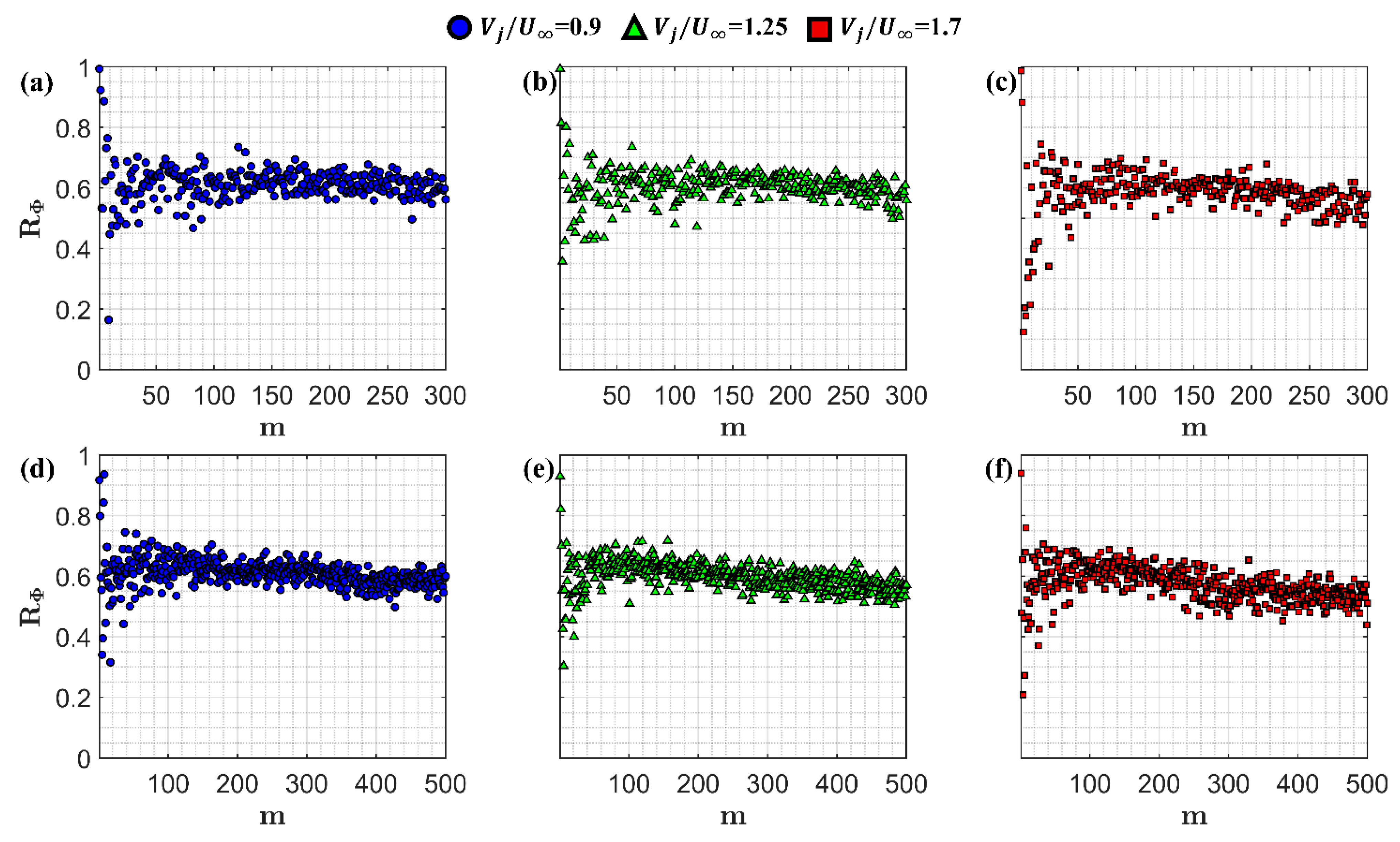
where and represent the eigenvectors of the composite and ‘true’ (here, measured) data, respectively, is the absolute value, and indicates the norm. The absolute value operator is imposed on the numerator to ensure no negative correlations are calculated, given that positive and negative signs on the spatial modes are accounted for by their matrix decomposition counterparts and have no physical meaning here. Assessment of the eigenvectors continues in Figure 7, which compares the spatial correlation provided in Equation (16) between the low-order modes of the composite and measured data for each velocity ratio tested.
The following observations are consistent and key trends across all available cases: within the first few modes, the correlation strength ‘switches’ between distinctly high values ( ≥ 0.7) to distinctly lower values (around < 0.45). Higher correlation values indicate that the complex flow field modes are well captured by superposition, while the lower values are likely a result of discrepancies in the hierarchical ranking of the unit and complex eigenvectors as observed earlier in Figure 6. After approximately the first 10 to 20 modes, the correlation values are defined within the range of approximately 0.45 ≤ ≤ 0.7, implying that the weighted superposition is strongly related to the low-order POD modes and their inherent dynamics. It is critical to note that this is consistent for both in-plane components of velocity, and . For the sake of brevity, the current investigation focuses on the in-plane velocity components only. However, it is not unreasonable to believe that these observations extend to other field variables that are functions of the current vector fields, e.g., pressure, vorticity.
4.5. Temporal Loadings
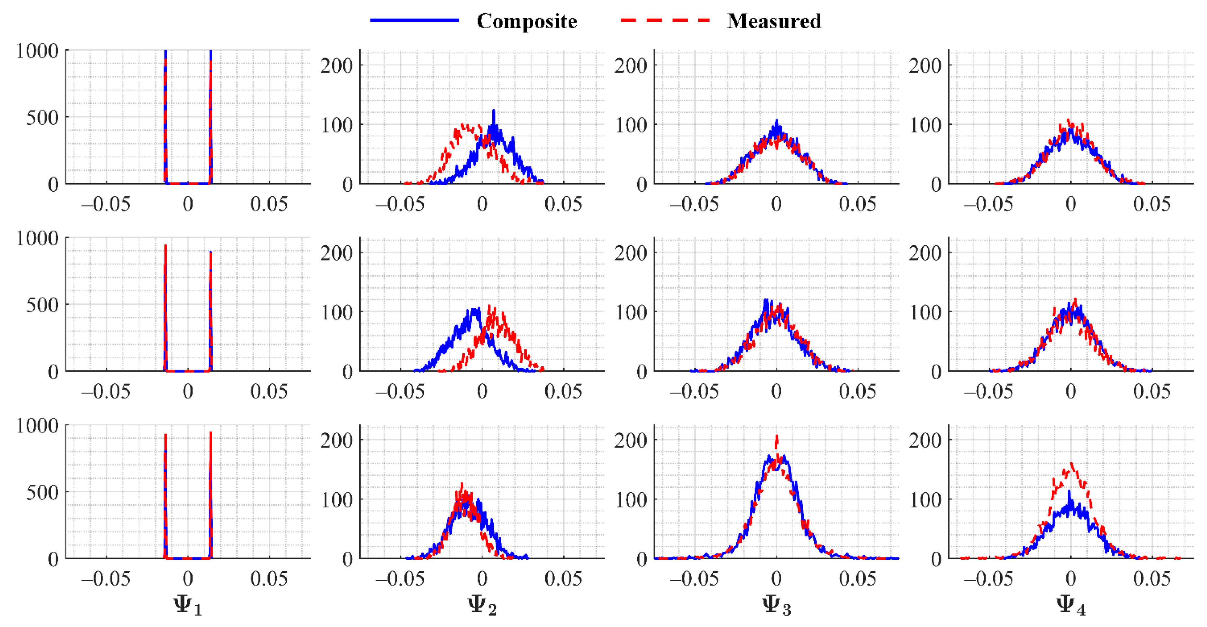
The final component of the decomposition, , quantifies the importance of each mode to an arbitrary instantaneous velocity field. More directly, each column of the matrix can be interpreted as the temporal loading of each mode onto the arbitrary instantaneous velocity field. Understanding the importance of each mode, and its relative loading, are critical to the prediction of large and small-scale spatial features [9,26]. It is useful to view histograms of these loadings to visualize similarities and differences in data sets, in this case by comparing the composite and measured data at a given velocity ratio as seen in Figure 8. For the sake of brevity, loadings for the fields are discussed, and those of . are excluded, though it is confirmed that similar observations apply to both components.
For the current application, the ideal outcome would seek to have the proposed weighting procedure replicate the physical behavior and kinetic energy of the system, in which the loading distributions would perfectly overlap. From Figure 8, the first modes, indicative of the average fields, yield distinct peaks with excellent overlap as expected. A far more critical evaluation is provided by the magnitudes and distributions of the temporal modes greater than . While general overlap is confirmed, two key differences can be found: first, separability, particularly in for the 0.9 and 1.25 cases and second, differences in magnitude, which are most evident in of 1.7. While physical interpretation is limited, it is well known that the POD allocates all temporal content of the input data into , and that the low-order reconstruction is heavily dependent on these temporal loadings. Future reconstruction schemes will likely seek to employ more robust computational methods to optimize transformation inputs and/or more readily account for the dominant frequencies of the system. While the POD’s optimality guarantees the identification of the most energetic modes, it does not distinguish between their frequencies, which may differ substantially in certain situations [2]. Higher-order improvements will thus benefit from also accounting for overlap in the temporal loadings, thereby fully constraining the POD parameters, towards optimal reconstruction schemes for repetitive flow geometries. There are several possible extensions in frequency-based decompositions as well, though this discussion is deferred to Section 5.
4.6. Projections
As a final assessment of the linearly weighted superposition, the composite data set is projected onto the measured one according to Equation (17).
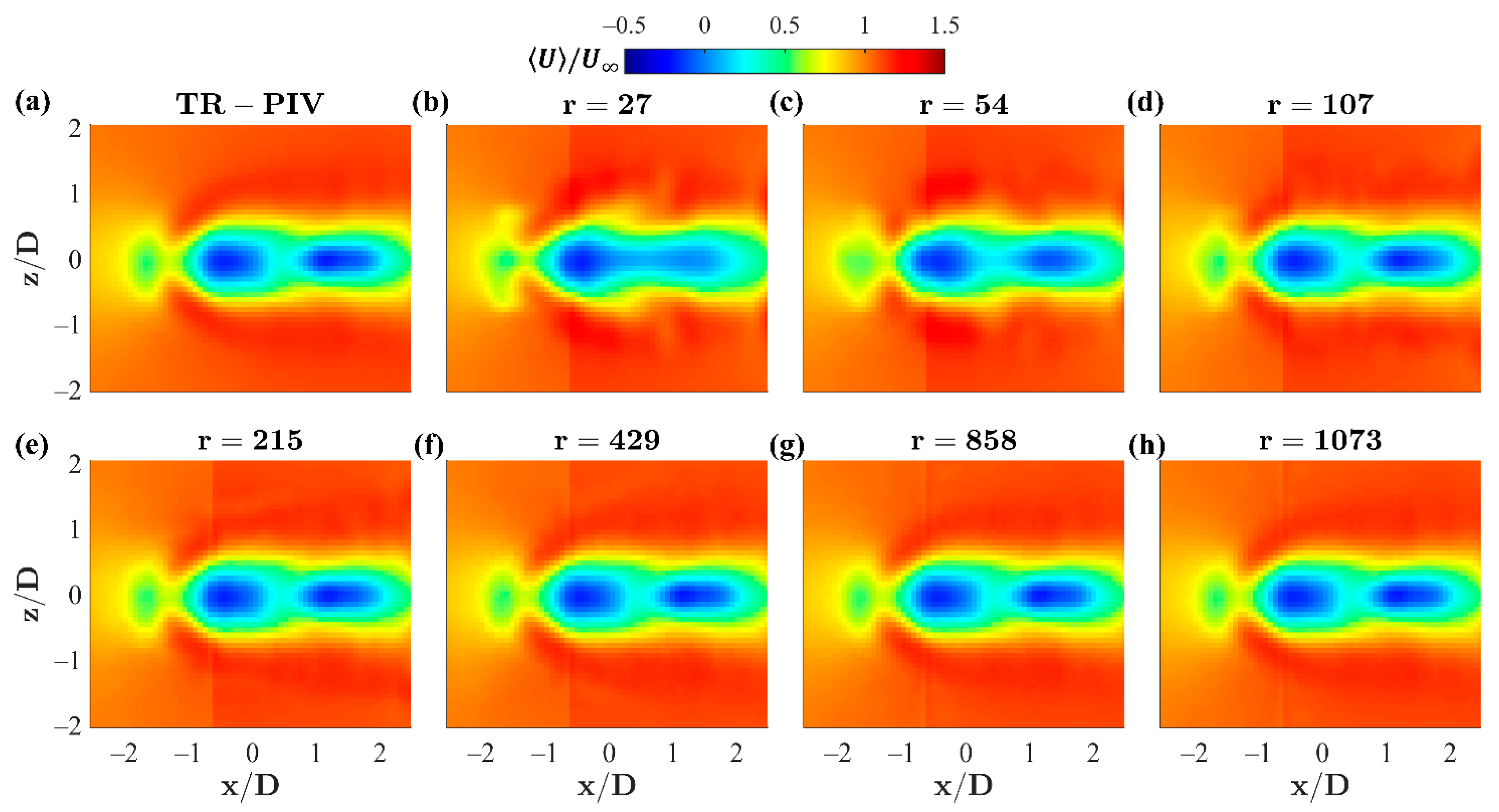
where is the projected approximation of the measured (‘true’) data, , as before. This example incorporates the time-averaged velocity field from the = 1.25 case, though this method could be applied to any instantaneous frame as well. The projection assesses the composite data set’s ability to replicate the true time-averaged behavior. This is accomplished only if the subspace of the composite data set includes a sufficient amount of similar or shared features as that of the time-averaged measurement data. The projection is presented in Figure 9 which displays the TR-PIV result for reference, and discrete truncation intervals of approximately 2.5, 5, 10, 20, 40, 80, and 100% of the total truncation () of the composite data set.
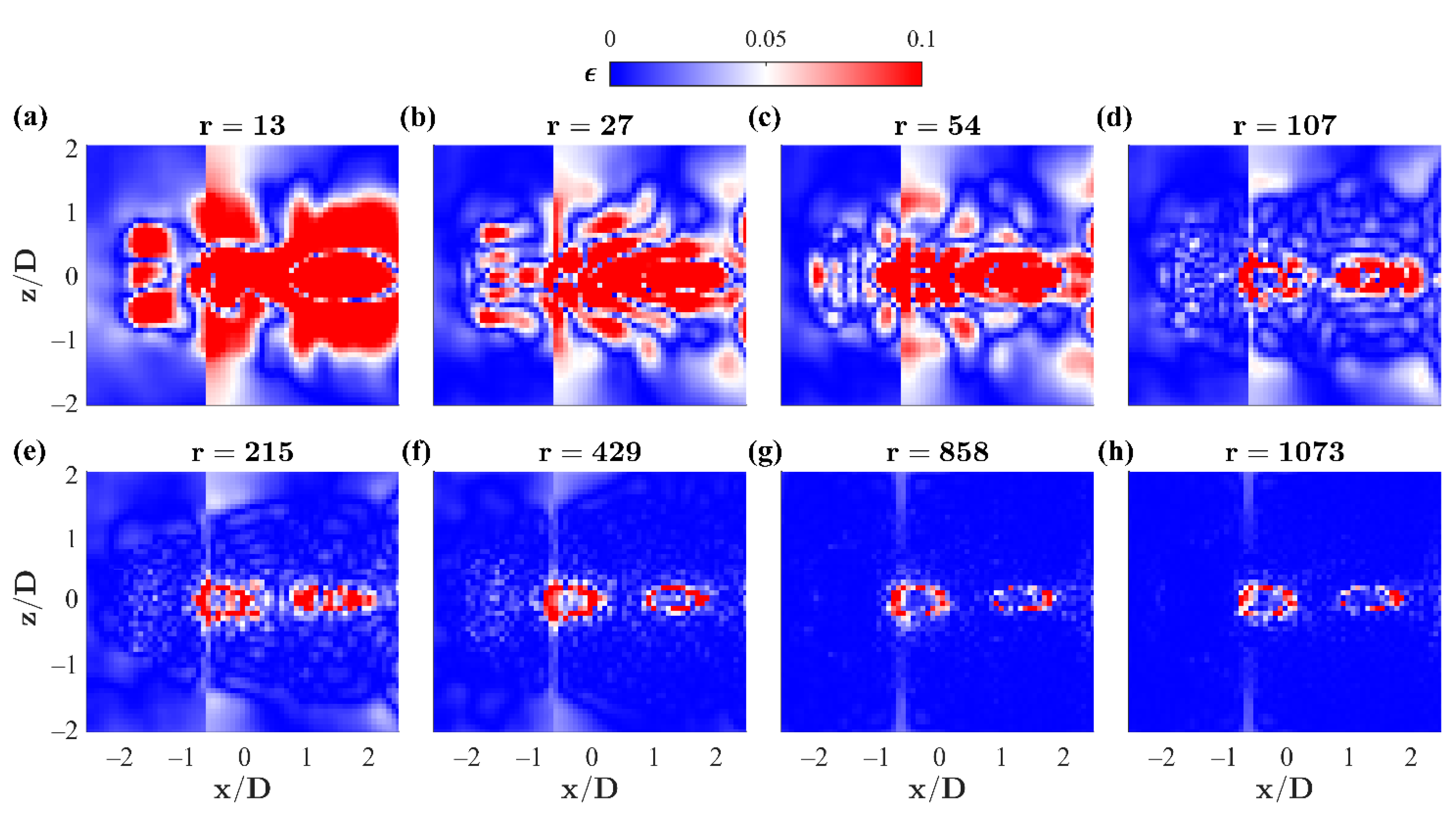
The projections reveal that there is indeed a sufficient overlap of features, physically understood as the effects of shear and rotation, between the composite and measured tandem jet flows to replicate the time-averaged field. By defining a relative error between the original TR-PIV data and the truncated data sets, according to Equation (18), this is further confirmed in Figure 10.
It is evident then, that across the fully truncated projection, the composite data set successfully projects the average flow field within 10% relative error, with the exception of the leading and middle jet penetration, seen as two roughly circular regions. It is reasonable to believe that the secondary effects of shielding, exhibited by an upstream jet on its downstream tandem neighbor, may be poorly captured in these regions by the unit flow and current weightings. Localized weightings may accommodate these effects, providing yet another avenue for development.
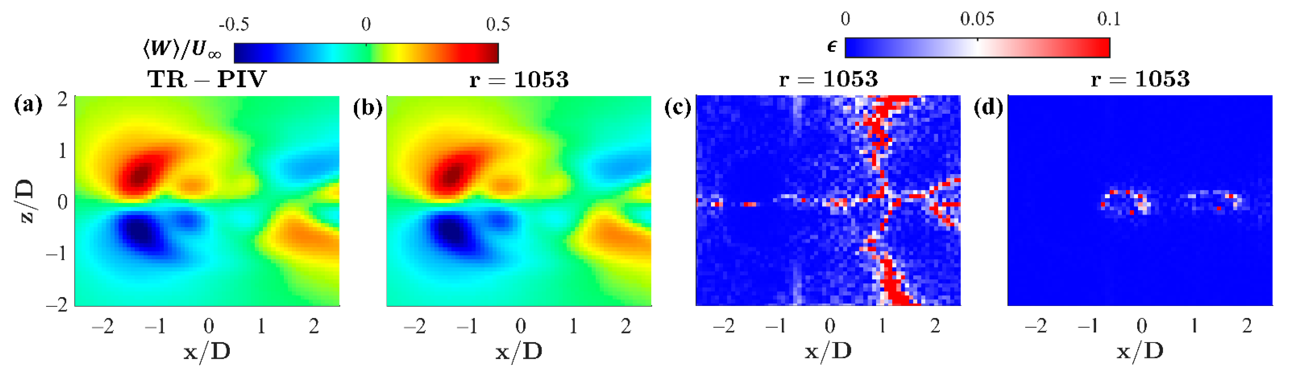
The procedure is briefly repeated here for the spanwise component, , and displayed in Figure 11.
In contrast to the streamwise component, the relative error for the component exhibits peak concentrations along 1.5 and is more sporadic than that found in Figure 10. This is a result of the smaller velocity values found in the non-dominant flow direction and relative error criteria in Equation (18), whose relative differences are exacerbated by smaller values in the denominator, . For reference, the spanwise relative error is non-dimensionalized by the time-averaged streamwise component, , in Figure 11d. Similar to the conclusions drawn from the streamwise component in Figure 10, the projection and corresponding relative error in Figure 11d confirms that the features are well represented, with the exception of the periphery of the leading and middle jet penetrations, here out of plane in the direction. The procedure relies heavily on the spatial and temporal resolution of the input data. This is customary for decomposition methods in general but is also crucial here for image editing and matrix transformations in order to successfully replicate the complex data. In addition to the linear weightings, the authors also considered stretching/compressing of the sub-domains to better replicate the wake motions of each jet in the complex flow. Again, the spatial grid resolution inhibited high modal correlation and adequate reconstruction of the measured complex flow field. The current TR-PIV benchmark data set consists of 2600 snapshots, sampled at 1 kHz, with 120 102 spatial grid points available. High-fidelity numerical simulation data, e.g., Large-Eddy Simulation, can provide much finer spatial detail, which may provide a fruitful next step in determining the grid sensitivity and relative error incurred by different unit placement configurations, i.e., stitched side by side, or as in the current benchmark, overlapping. Nonetheless, the proposed method is a testament to ‘error vs. effort’: the ability of the composite data set to capture the spatial, energetic, and temporal scales of the ‘true’ data set with minimal a priori expertise, user and computational expense, and low memory storage has several important consequences on the future understanding and analysis of fluid mechanics.
While several possible avenues exist for more efficient and robust reconstructions, the authors provide only a brief overview here for potential improvements surrounding the choice of input data, weighting strategy, and decomposition technique. As alluded to in 1.0 Introduction and motivation, an important observation of the proposed weighted superposition and the well-established POD are that both techniques are linear representations of the primitive data, i.e., the velocity fields. The success of the current weighted superposition, as applied directly to these velocity fields, suggests that with improved data resolution and larger fields of view, the POD unit flow eigenvectors may be used directly, in place of the unit flow primitive data, to reconstruct complex flow fields. These unit eigenvectors would then be subject to similar image editing, matrix transformations, and optimized weightings according to the ‘true’ complex mode shapes. The implication here is that these generalized mode shapes could be scaled to a variety of geometries, flow types, and non-dimensional parameters in their respective class of flows, via a ‘library’ of weightings. This proposed method holds significant potential for reduced computational expense and scaling of complicated industrial flow features. As discussed for the current benchmark, experiments are typically limited by their field of view and testing ranges. As such, these efforts may benefit more directly from high-fidelity numerical simulations.
5. Discussion
A linearly weighted superposition method has been introduced that seeks to replicate key aspects of the spatio-temporal behavior of complex fluid flow data from its constituent unit flow feature(s). The qualified success of linear potential flow theory and linear decomposition methods such as proper orthogonal decomposition (POD) provide motivation and guidance for the present approach. In order to achieve the stated objective, the unit feature(s) are processed through a combination of empirical image editing, conventional matrix transformations, and optimized weightings to produce an artificial composite representation of a ‘true’ experimentally measured or numerically simulated complex data field. Weightings are optimized using the ‘true’ data set and are then multiplied to each of the prescribed sub-domains, the sum of which yields the composite flow field. POD is applied to the composite data set and the ‘true’ data set, thereby separating their spatial and temporal content via their corresponding eigenvalues for comparison and evaluation of the proposed method. The methodology is formulated and examined using previously vetted experimental data [15].
The benchmark data set consists of time-resolved particle image velocimetry (TR-PIV) cross-sectional measurements of a single and triple tandem jet array, constituting the unit and complex flows, respectively. The single jet in crossflow is known to exhibit markedly different boundary layer interactions, pressure gradients, turbulence, and vortex formations as a function of velocity or momentum ratio. Universal scaling laws have proven elusive, and the introduction of additional jets only complicates their interactions further, making these data sets an excellent candidate for the proposed method. Copies of the single jet velocity profile are cropped into three separate positions based on the axial centerline of each tandem jet, multiplied by their respective optimal weightings, and then summed to form the composite representation of the ‘true’ measured tandem jet profiles. An optimal weighting combination is determined for both in-plane velocity components at three distinct jet to crossflow velocity ratios in the range of 0.9 to 1.7. Composite eigenvalues and cumulative energy distributions have faithfully reproduced those of the measured tandem jet data, with only slight overprediction. Based on an optimal hard threshold, the composite profiles also require less modes than the measurement data, implying that the method may have a significant contribution in compressing complex data sets. Low-order eigenvectors suggest good (~0.7 or higher) correlation and capture the large-scale flow features produced by shear and rotation within the flow, with weaker representation of the smaller-scale eddies. Similarities and differences in the temporal loadings are also assessed for completeness and as another possible avenue for improved reconstruction of complex flows from their unit basis/bases. The assessment concludes with the projection of composite data sets onto their corresponding measured time-averaged velocity profiles. The truncated modes capture all major features of the bulk flow within 10% relative error with the exception of small regions found along the periphery of the jet cores’ penetration through the plane. From this benchmark investigation, it is evident that the proposed methodology’s composite flow representations accurately reconstruct the large-scale features of their analogous complex flow fields.
The critical tasks described here are concerned with feature extraction, shape optimization, and dimensionality reduction, all of which are addressed within the larger framework of machine learning (ML). It is clear that future improvements to complex flow reconstruction should seek more advanced ML algorithms for these tasks. The current weightings employ quadratic programming to solve the objective function, providing uniform scalar weightings between the composite and ‘true’ data sets, here, the velocity fields. Although empirical, these weightings served the current motive of viable reconstruction of complex flows. Supervised learning methods will likely best serve the optimal localized weightings, with neural networks being an attractive candidate [46,47,48,49]. Regarding dimensionality reduction techniques, the POD is an energy-based decomposition, and as alluded to in Section 4.5, several frequency-based, or emerging hybrid decompositions, are plausible with attractive candidates including the dynamic modal decomposition (DMD) [45,50,51] and multi-scale proper orthogonal decomposition (mPOD) [2], respectively. A critical factor towards the maturity of such candidates is establishing the degree of resolution needed to accurately compute the associated coherent structures [52]. More refined decompositions will no doubt provide additional means of identifying and replicating the spatial and temporal content of a given complex data set. It is evident then, that a truly robust complex flow field reconstruction strategy will require significant data-driven efforts within the fluid mechanics and ML communities, providing several exciting avenues for improved understanding, modeling, optimization, and control of complex fluid flows, and the wider class of dynamical systems.
Author Contributions
Conceptualization, P.J.K., M.L.K., and S.S.G.; methodology, P.J.K. and S.S.G.; software, P.J.K.; validation, P.J.K.; formal analysis, P.J.K.; investigation, P.J.K.; resources, M.L.K.; data curation, P.J.K.; writing—original draft preparation, P.J.K., M.L.K., and S.S.G.; writing—review and editing, P.J.K., M.L.K., and S.S.G.; visualization, P.J.K.; supervision, M.L.K. and S.S.G.; project administration, M.L.K.; funding acquisition, M.L.K. All authors have read and agreed to the published version of the manuscript.
Funding
This research was funded by the Nuclear Energy University Program (NEUP) through the following projects: NEUP 12-3582 entitled “Experimentally Validated Numerical Models of Non-Isothermal Turbulent Mixing in High Temperature Reactors”; NEUP 15-8627 entitled “Experimental Validation Data and Computational Models for Turbulent Mixing of Bypass and Coolant Jet Flows in Gas-Cooled Reactors”.
Acknowledgments
The authors thank the reviewers and editor for their comments and suggestions during the review of this manuscript.
Conflicts of Interest
The authors declare no conflict of interest.
References
- Brunton, S.L.; Noack, B.R. Closed-Loop Turbulence Control: Progress and Challenges. Appl. Mech. Rev. 2015, 67. [Google Scholar] [CrossRef]
- Mendez, M.A.; Balabane, M.; Buchlin, J.-M. Multi-scale proper orthogonal decomposition of complex fluid flows. J. Fluid Mech. 2019, 870, 988–1036. [Google Scholar] [CrossRef] [Green Version]
- Taneda, S. Experimental investigation of the wakes behind cylinders and plates at low Reynolds numbers. J. Phys. Soc. Jpn. 1956, 11, 302–307. [Google Scholar] [CrossRef]
- Coutanceau, M.; Bouard, R. Experimental determination of the main features of the viscous flow in the wake of a circular cylinder in uniform translation. Part 1. Steady flow. J. Fluid Mech. 2006, 79, 231–256. [Google Scholar] [CrossRef]
- Rosenhead, L. The formation of vortices from a surface of discontinuity. Proc. R. Soc. London. Ser. A, Contain. Pap. A Math. Phys. Character 1931, 134, 170–192. [Google Scholar]
- Winant, C.D.; Browand, F.K. Vortex pairing: The mechanism of turbulent mixing-layer growth at moderate Reynolds number. J. Fluid Mech. 1974, 63, 237–255. [Google Scholar] [CrossRef]
- Adrian, R.J.; Christensen, K.T.; Liu, Z.-C. Analysis and interpretation of instantaneous turbulent velocity fields. Exp. Fluids 2000, 29, 275–290. [Google Scholar] [CrossRef]
- Taira, K.; Hemati, M.S.; Brunton, S.L.; Sun, Y.; Duraisamy, K.; Bagheri, S.; Dawson, S.T.M.; Yeh, C.-A. Modal Analysis of Fluid Flows: Applications and Outlook. AIAA J. 2020, 58, 998–1022. [Google Scholar] [CrossRef]
- Taira, K.; Brunton, S.L.; Dawson, S.T.M.; Rowley, C.W.; Colonius, T.; McKeon, B.J.; Schmidt, O.T.; Gordeyev, S.; Theofilis, V.; Ukeiley, L.S. Modal Analysis of Fluid Flows: An Overview. AIAA J. 2017, 55, 4013–4041. [Google Scholar] [CrossRef] [Green Version]
- Pollard, A.; Castillo, L.; Danaila, L.; Glauser, M. Whither Turbulence and Big Data in the 21st Century? Springer: Berlin/Heidelberg, Germany, 2016. [Google Scholar]
- Schlicting, H.; Gersten, K. Boundary-Layer Theory, 7th ed.; Springer: Berlin/Heidelberg, Germany, 1979. [Google Scholar]
- Bradshaw, P. An Introduction to Turbulence and Its Measurement: Thermodynamics and Fluid Mechanics Series; Elsevier: Amsterdam, The Netherlands, 1971. [Google Scholar]
- Pope, S.B. Turbulent Flows; Cambridge University Press: Cambridge, UK, 2000. [Google Scholar]
- Katz, J.; Plotkin, A. Low-Speed Aerodynamics; Cambridge University Press: Cambridge, UK, 2001; Volume 13. [Google Scholar]
- Kristo, P.J.; Kimber, M.L. Time-resolved particle image velocimetry measurements of a tandem jet array in a crossflow at low velocity ratios. Exp. Fluids 2021, 62. [Google Scholar] [CrossRef]
- Loève, M. Probability Theory I.; Springer: New York, NY, USA, 1977. [Google Scholar]
- Lumley, J.L. The structure of inhomogeneous turbulent flows. In Atmos. Turbul. Radio Wave Propag; Yaglom, A.M., Tatarski, V.I., Eds.; Nauca: Moscow, Russia, 1967. [Google Scholar]
- Holmes, P.; Lumley, J.L.; Berkooz, G. Turbulence, Coherent Sturctures, Dynamical Systems, and Symmetry, 1st ed.; Cambridge University Press: Cambridge, UK, 1996. [Google Scholar]
- Berkooz, G.; Holmes, P.; Lumley, J.L. The proper orthogonal decomposition in the analysis of turbulent flows. Annu. Rev. Fluid Mech. 1993, 25, 539–575. [Google Scholar] [CrossRef]
- Holmes, P.; Lumley, J.L.; Berkooz, G.; Rowley, C.W. Turbulence, Coherent Structures, Dynamical Systems and Symmetry, 2nd ed.; Cambridge University Press: Cambridge, UK, 2012. [Google Scholar]
- Rowley, C.W.; Dawson, S.T.M. Model Reduction for Flow Analysis and Control. Annu. Rev. Fluid Mech. 2017, 49, 387–417. [Google Scholar] [CrossRef] [Green Version]
- Brunton, S.L.; Noack, B.R.; Koumoutsakos, P. Machine Learning for Fluid Mechanics. Annu. Rev. Fluid Mech. 2020, 52, 477–508. [Google Scholar] [CrossRef] [Green Version]
- Chomaz, J.-M. Global Instabilties in Spatially Developing Flows: Non-Normality and Nonlinearity. Annu. Rev. Fluid Mech. 2005, 37, 357–392. [Google Scholar] [CrossRef] [Green Version]
- Bishop, C.M. Pattern Recognition and Machine Learning, 1st ed.; Springer: Berlin/Heidelberg, Germany, 2006. [Google Scholar]
- Theodoridis, S.; Koutroumbas, K. Pattern Recognition, 2nd ed.; Elsevier: Amsterdam, The Netherlands, 2003. [Google Scholar]
- Brunton, S.L.; Kutz, J.N. Data-Driven Science and Engineering: Machine Learning, Dynamical Systems, and Control; Cambridge University Press: Cambridge, UK, 2019. [Google Scholar]
- Golub, G.; Kahan, W. Calculating the singular values and pseudo-inverse of a matrix. J. Soc. Ind. Appl. Math. Ser. B Numer. Anal. 1965, 2, 205–224. [Google Scholar] [CrossRef]
- Stewart, G.W. On the early history of the singular value decomposition. SIAM Rev. 1993, 35, 551–566. [Google Scholar] [CrossRef] [Green Version]
- Eckart, C.; Young, G. The approximation of one matrix by another of lower rank. Psychometrika 1936, 1, 211–218. [Google Scholar] [CrossRef]
- Sirovich, L. Turbulence and the dynamics of coherent structures. I. Coherent structures. Q. Appl. Math. 1987, 45, 561–571. [Google Scholar] [CrossRef] [Green Version]
- Sirovich, L. Turbulence and the dynamics of coherent structures. II. Symmetries and transformations. Q. Appl. Math. 1987, 45, 573–582. [Google Scholar] [CrossRef] [Green Version]
- Sirovich, L. Turbulence and the dynamics of coherent structures. III. Dynamics and scaling. Q. Appl. Math. 1987, 45, 583–590. [Google Scholar] [CrossRef] [Green Version]
- Gavish, M.; Donoho, D.L. The Optimal Hard Threshold for Singular Values is 4/√3. IEEE Trans. Inf. Theory 2014, 60, 5040–5053. [Google Scholar] [CrossRef]
- Gill, P.E.; Murray, W.; Wright, M.H. Practical Optimization; Academic Press: London, UK, 1981. [Google Scholar]
- Jiménez, J. Coherent structures in wall-bounded turbulence. J. Fluid Mech. 2018, 842. [Google Scholar] [CrossRef] [Green Version]
- Jiménez, J.; Moin, P. The minimal flow unit in near-wall turbulence. J. Fluid Mech. 1991, 225, 213–240. [Google Scholar] [CrossRef] [Green Version]
- Muralidhar, S.D.; Podvin, B.; Mathelin, L.; Fraigneau, Y. Spatio-temporal proper orthogonal decomposition of turbulent channel flow. J. Fluid Mech. 2019, 864, 614–639. [Google Scholar] [CrossRef] [Green Version]
- Winter, M.; Barbert, T.J.; Everson, R.M.; Sirovich, L. Eigenfunction analysis of turbulent mixing phenomena. AIAA J. 1992, 30, 1681–1688. [Google Scholar] [CrossRef]
- Meyer, K.E.; Pedersen, J.M.; ÖZcan, O. A turbulent jet in crossflow analysed with proper orthogonal decomposition. J. Fluid Mech. 2007, 583, 199–227. [Google Scholar] [CrossRef] [Green Version]
- Surya Prakash, R.; Sinha, A.; Tomar, G.; Ravikrishna, R.V. Liquid jet in crossflow—Effect of liquid entry conditions. Exp. Therm. Fluid Sci. 2018, 93, 45–56. [Google Scholar] [CrossRef]
- Cavar, D.; Meyer, K.E. LES of turbulent jet in cross flow: Part 2—POD analysis and identification of coherent structures. Int. J. Heat Fluid Flow 2012, 36, 35–46. [Google Scholar] [CrossRef]
- Wu, Z.; Laurence, D.; Utyuzhnikov, S.; Afgan, I. Proper orthogonal decomposition and dynamic mode decomposition of jet in channel crossflow. Nucl. Eng. Des. 2019, 344, 54–68. [Google Scholar] [CrossRef]
- Mahesh, K. The Interaction of Jets with Crossflow. Annu. Rev. Fluid Mech. 2013, 45, 379–407. [Google Scholar] [CrossRef]
- Kristo, P.J.; Sohail, S.; Reed, R.S.; Kimber, M.L. Low speed wind tunnel flow diagnostics and benchmark cases for thermal fluids CFD validation efforts. In Proceedings of the ASME 2021 Fluids Engineering Division Summer Meeting (FEDSM2021), Virtual, 10–12 August 2021. [Google Scholar]
- Kutz, J.N.; Brunton, S.L.; Brunton, B.W.; Proctor, J.L. Dynamic Mode Decomposition: Data-Driven Modeling of Complex Systems; Society for Industrial and Applied Mathematics: University City, PA, USA, 2016. [Google Scholar]
- Grossberg, S. Nonlinear neural networks: Principles, mechanisms, and architectures. Neural Netw. 1988, 1, 17–61. [Google Scholar] [CrossRef] [Green Version]
- Krizhevsky, A.; Sutskever, I.; Hinton, G.E. Imagenet classification with deep convolutional neural networks. Adv. Neural Inf. Process. Syst. 2012, 25, 1097–1105. [Google Scholar] [CrossRef]
- Goodfellow, I.; Bengio, Y.; Courville, A. Deep Learning; MIT Press: Cambridge, MA, USA, 2016. [Google Scholar]
- Taghizadeh, S.; Witherden, F.D.; Girimaji, S.S. Turbulence closure modeling with data-driven techniques: Physical compatibility and consistency considerations. New J. Phys. 2020, 22, 093023. [Google Scholar] [CrossRef]
- Proctor, J.L.; Brunton, S.L.; Kutz, J.N. Dynamic Mode Decomposition with Control. SIAM J. Appl. Dyn. Syst. 2016, 15, 142–161. [Google Scholar] [CrossRef] [Green Version]
- Tu, J.H.; Rowley, C.W.; Luchtenburg, D.M.; Brunton, S.L.; Nathan Kutz, J. On dynamic mode decomposition: Theory and applications. J. Comput. Dyn. 2014, 1, 391–421. [Google Scholar] [CrossRef] [Green Version]
- Fowler, T.S.; Witherden, F.D.; Girimaji, S.S. Partially-averaged Navier–Stokes simulations of turbulent flow past a square cylinder: Comparative assessment of statistics and coherent structures at different resolutions. Phys. Fluids 2020, 32. [Google Scholar] [CrossRef]
Figure 1.
(a) Composite sub-domains extracted from the single jet velocity field data, (b) clear depiction of each sub-domain and appended null matrices, and (c) representation of the overlaid sub-domains to approximate the tandem jet array’s experimentally measured flow physics. Color legend: black— ‘true’ measurement data, blue—sub-domain of jet 1, green—sub-domain of jet 2, and red—sub-domain of jet 3 based on current available field of view.

Figure 2.
Test section including (a) side view depicting plane and (b) top view depicting plane. Reproduced with permission from Kristo and Kimber, Time-resolved particle image velocimetry measurements of a tandem jet array in a crossflow at low velocity ratios [15]; published by Springer Nature, 2021.

Figure 3.
Instantaneous velocity magnitudes with vector components and . Rows depict (a–c) single and (d–f) triple jets with white circles and columns (a,d), (b,e), and (c,f) correspond to 0.9, 1.25, 1.7, respectively. Reproduced with permission from Kristo and Kimber, Time-resolved particle image velocimetry measurements of a tandem jet array in a crossflow at low velocity ratios [15]; published by Springer Nature, 2021.

Figure 4.
Time-averaged velocity magnitudes with velocity streamlines. Rows depict (a–c) single and (d–f) triple jets with white circles and columns (a,d), (b,e), and (c,f) correspond to = 0.9, 1.25, 1.7, respectively. Reproduced with permission from Kristo and Kimber, Time-resolved particle image velocimetry measurements of a tandem jet array in a crossflow at low velocity ratios [15]; published by Springer Nature, 2021.

Figure 5.
Low-order eigenvalue magnitudes and cumulative energy distribution sums for velocity components (a–c) and (d–f) at each velocity ratio ((a,d), (b,e), and (c,f) correspond to = 0.9, 1.25, 1.7, respectively). Describes the kinetic energy content of each POD mode for comparison between composite and experimentally measured tandem jets.

Figure 6.
Low-order POD velocity mode shapes for the = 1.25 for the (a) composite and (b) measured data sets and the (c) composite and (d) measured data sets. Relative percent energies are displayed in the bottom left corner of each contour.
Figure 6.
Low-order POD velocity mode shapes for the = 1.25 for the (a) composite and (b) measured data sets and the (c) composite and (d) measured data sets. Relative percent energies are displayed in the bottom left corner of each contour.

Figure 7.
Composite-measured eigenvector correlations for the low-order modes of (a–c) and (d–f) velocity fields, respectively, at each velocity ratio.
Figure 7.
Composite-measured eigenvector correlations for the low-order modes of (a–c) and (d–f) velocity fields, respectively, at each velocity ratio.

Figure 8.
Histograms of the temporal loading distributions for composite and measured data for the first four modes of each velocity ratio (rows, top to bottom: = 0.9, 1.25, 1.7).
Figure 8.
Histograms of the temporal loading distributions for composite and measured data for the first four modes of each velocity ratio (rows, top to bottom: = 0.9, 1.25, 1.7).

Figure 9.
Contours of the composite data set decomposition projected onto the time-averaged velocity, measurement data for = 1.25 as a function of increasing modal contributions. The (a) TR-PIV time average of the complex flow is included for comparison against the fully truncated composite projection of the unit flow with approximately (b) 2.5%, (c) 5%, (d) 10%, (e) 20%, (f) 40%, (g) 80%, and (h) 100% of the truncated modes.

Figure 10.
Relative error, , contours of projected composite data decomposition onto the measurement data time-averaged streamwise velocity, , for = 1.25 as a function of increasing modal contributions including approximately (a) 1.25%, (b) 2.5%, (c) 5%, (d) 10%, (e) 20%, (f) 40%, (g) 80%, and (h) 100% of the truncated modes.

Figure 11.
= 1.25 case time-averaged spanwise velocity, , contours of (a) measurement data and (b) projected composite data, as well as relative error, , contours normalized by (c) measured , and (d) measured .
Figure 11.
= 1.25 case time-averaged spanwise velocity, , contours of (a) measurement data and (b) projected composite data, as well as relative error, , contours normalized by (c) measured , and (d) measured .


Table 1.
Optimal velocity component weightings for each composite jet at each jet to crossflow velocity ratio.
Table 1.
Optimal velocity component weightings for each composite jet at each jet to crossflow velocity ratio.
| Jet 1 | Jet 2 | Jet 3 | ||||
|---|---|---|---|---|---|---|
| 0.9 | 0.9589 | 0.8089 | 0.0000 | 0.1911 | 0.0411 | 0.0000 |
| 1.25 | 0.9474 | 0.9094 | 0.0526 | 0.0906 | 0.0000 | 0.0000 |
| 1.7 | 0.9382 | 0.9689 | 0.0618 | 0.03111 | 0.0000 | 0.0000 |
Table 2.
Optimal hard truncation values for each velocity component, and , corresponding to each case. Measured and composite data for the tandem jets are listed with and without parenthesis, respectively.
Table 2.
Optimal hard truncation values for each velocity component, and , corresponding to each case. Measured and composite data for the tandem jets are listed with and without parenthesis, respectively.
| Vj/U∞ | U(x,z,t) | W(x,z,t) | ||
|---|---|---|---|---|
| r | τ | r | τ | |
| 0.9 | 1088 (1095) | 0.81 (0.88) | 1052 (1065) | 0.59 (0.91) |
| 1.25 | 1073 (1227)) | 1.06 (1.12) | 1053 (1172) | 0.88 (1.16) |
| 1.7 | 1070 (1269) | 1.17 (1.51) | 1030 (1207) | 1.14 (1.58) |
Publisher’s Note: MDPI stays neutral with regard to jurisdictional claims in published maps and institutional affiliations. |
© 2021 by the authors. Licensee MDPI, Basel, Switzerland. This article is an open access article distributed under the terms and conditions of the Creative Commons Attribution (CC BY) license (https://creativecommons.org/licenses/by/4.0/).
Share and Cite
MDPI and ACS Style
Kristo, P.J.; Kimber, M.L.; Girimaji, S.S. Towards Reconstruction of Complex Flow Fields Using Unit Flows. Fluids 2021, 6, 255. https://0-doi-org.brum.beds.ac.uk/10.3390/fluids6070255
AMA Style
Kristo PJ, Kimber ML, Girimaji SS. Towards Reconstruction of Complex Flow Fields Using Unit Flows. Fluids. 2021; 6(7):255. https://0-doi-org.brum.beds.ac.uk/10.3390/fluids6070255
Chicago/Turabian StyleKristo, Paul J., Mark L. Kimber, and Sharath S. Girimaji. 2021. "Towards Reconstruction of Complex Flow Fields Using Unit Flows" Fluids 6, no. 7: 255. https://0-doi-org.brum.beds.ac.uk/10.3390/fluids6070255