1. Introduction
In modern research, non-Newtonian fluids have great significance. The rheological attributes of non-Newtonian type fluids cannot be well illustrated by the famous Navier–Stokes equation only. Therefore, scientists proposed several models to portray the characteristics of non-Newtonian fluids. In 1929, Williamson proposed a model for non-Newtonian fluids that illustrates the rheological attributes of non-Newtonian type fluids. In recent years, many scientists worked on the Williamson model to study the behavior of non-Newtonian fluids. Kebede et al. [
1] recently reported the heat and mass transport in Williamson nanofluids. Kumar et al. [
2] investigated the MHD fluid flow bounded by a curved sheet for the Williamson fluid model. They found increasing outcome of rising curvature parameter on velocity and decrement in it is seen for large values of the Williamson and magnetic parameters. In a study, Nadeem et al. [
3] analyzed the flow bounded by a stretching sheet for Williamson type fluid model and discussed the results graphically. Nadeem et al. [
4] investigated the flow of Williamson-type nanofluid determined by stretching sheet by presenting a new form of governing equations. Salahuddin et al. [
5] analyzed the Induced MHD impact on exponentially varying viscosity of Williamson fluid flow with variable conductivity and diffusivity. Ibrahim [
6] used the Williamson model to tackle the MHD flow over a stretchable cylinder using the porous medium. Iqbal et al. [
7] recently analyzed the Williamson fluid flow in a cylinder by considering an exponentially stretching sheet. They presented the effects on velocity and skin friction graphically by adopting the shooting technique. Panezai et al. [
8] numerically investigated the heat transfer characteristics of Williamson fluid over a porous Wedge. Salahuddin et al. [
9] studied the boundary layer phenomena of Williamson-type fluid with slip conditions over a stretching cylinder.
Heat transfer flows with the porous surface are of considerable interest due to their advanced engineering applications and their frequent use in industrial technology and power generation systems. Food processing, cooling towers, and the distribution of temperature are the leading examples. Kairi et al. [
10] reported the effect of melting on mixed convection heat and mass transfer in a non-Newtonian-fluid-saturated, non-Darcy porous medium. Bestman [
11] explored the heat and mass flux accompanying the free convection in the boundary layer flow using the porous medium. Lakshmi et al. [
12] reported mixed convection type stagnation point fluid flow analysis using a stretching type porous surface. Ambreen et al. [
13] reported an analytic investigation on boundary layer phenomena and heat flux, specifically using a rotating disk with porous attributes. In a study, Rasool et al. [
14] reported the entropy (disorder) consequences and the high impact of a second-order chemical reaction in a nanofluid based on the Darcy model known for porous medium using a non-linear stretching surface. Shafiq et al. [
15] presented the importance of convective boundary and thermal slip in a three-dimensional and rotating disk (porous medium). Reddy et al. [
16] presented numerical results for the boundary layer phenomena of a nanofluid using a porous medium on an exponentially stretching sheet.
Magnetohydrodynamics (MHD) is the study of fluid behavior in the presence of electric and magnetic fields. MHD plays a significant role in biomedical and industrial sciences [
17]. Some applications of MHD are magnetic drug targeting, cancer tumor treatment, magnetic devices for cell separation, magnetic endoscopy, and adjusting blood flow during surgery. Much advancement is observed in research related to MHD flows over a stretching surface in the literature. Jabeen et al. [
18] considered a porous surface to study the effects of MHD boundary layer flow over a stretching surface and observed that Maxwell fluid has a high thermal conductivity rate compared to other non-Newtonian fluid models. Rasool et al. [
19] analyzed the high impact of Darcy medium (porous medium) on MHD nanofluid bounded by a stretching (non-linear) surface. In another study, the authors Rasool et al. [
20] use the famous SPECTRAL method to figure out the impact of EMHD by a vertical Riga plate in a second-grade type nanofluid. Akbar et al. [
21] numerically investigated the MHD flow of second-grade fluids in a porous medium with prescribed vorticity. Aurangzaib et al. [
22] reported the unsteady MHD type mixed convective flow based on a micropolar porous surface.
In recent research, the boundary layer flow over stretching curved/flat surfaces has attracted much attention for specific reasons, such as their extensive industry and engineering sector applications. Many fundamental processes involve condensation, drawing of wires, metal extrusion, rolling, fiber spinning, and polymer sheet extrusion, showing the essential applications of stretching surfaces in industries. Sakiadis [
23] derived the fundamental differential equations for the boundary layer type theory of continuous solid surfaces for both the laminar and turbulent flow. Crane [
24] proposed an exact solution for surface friction and thermal conductivity for the flow past a stretching surface. Gupta et al. [
25] investigated mass, heat, and momentum over a stretching surface in the boundary layer subject to blowing and suction. Okechi et al. [
26] investigated the fluid flow phenomena along exponential and stretching curved surface. Kumar et al. [
27] analyzed the MHD fluid flow of micropolar fluid passed over an exponential and stretching carved surface. Nayak [
28] investigated MHD convective flow to study the impact of thermal diffusion via an exponentially stretching sheet and proposed an iterative solution by using the R.K. method and shooting technique. Jalil and Asghar [
29] presented a pioneer work by discussing exponential stretching using Lie group analysis for the first time. They used the perturbation method to extend their investigation for shear-thinning fluids. Sanni et al. [
30] blended the stretching surface and curved surface concepts to study viscous fluid flow. Recently, Ahmed and Akbar [
31] numerically investigated the MHD Williamson nanofluid flow over an exponentially stretching surface.
Motivated by the above literature review, it has been observed that no study is so far reported which investigates the heat transfer characteristics of Williamson type fluid flow via an exponentially stretching curved surface in the presence of variable thermal conductivity. The prime aim of the present investigation is to study the heat flow of Williamson fluids over an exponentially stretching porous curved surface with a heat source. With the help of suitable similarity transformation, the governing PDEs are converted into ODEs. The highly non-linear ODEs are solved numerically by using Matlab code bvp4c. The impact of the curvature parameter, magnetic number, suction/injection parameter, permeability parameter, Prandtl factor, Eckert factor, non-linear radiation parameter, buoyancy parameter, temperature ratio parameter, Williamson fluid parameter, thermal conductivity parameter on velocity, pressure, and temperature profiles are observed by the plotted graphs. The variation in the skin friction and Nusselt number due to the involved physical parameters are observed through tables.
2. Problem Description
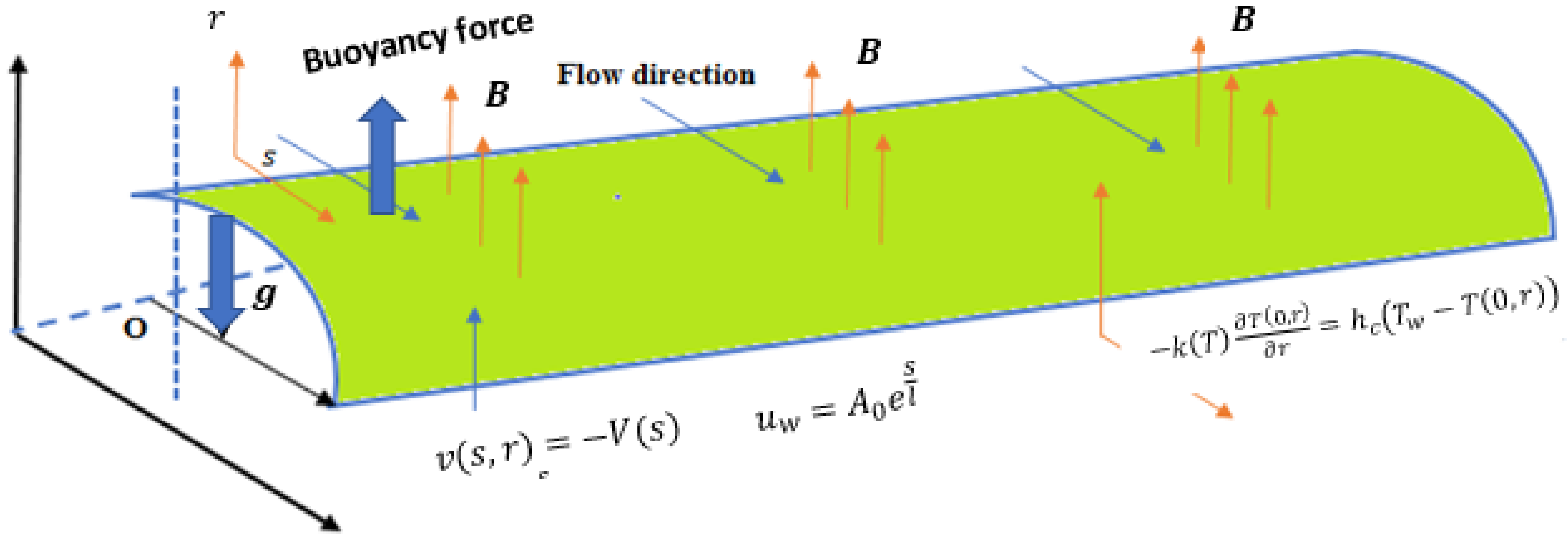
Here we have considered a steady, incompressible, laminar two-dimensional mixed convective Williamson type fluid flow under the impact of MHD to observe the attributes of the heat transfer mechanism along an exponentially stretching porous curved surface. Considering the coordinate system
where
is assumed along the fluid flow direction, and the
-axis is taken orthogonally to the flow, let R be the total radius of the curved surface. The physical scenario and the setup of coordinates are portrayed in
Figure 1. The velocity field (stretching) of the surface is
, which is taken along the
-direction. An exponentially varying magnetic field
is taken in the radial direction whereas, the temperature adjacent to the surface is
. Under the above assumptions, the flow equations following [
2,
27] are given below:
Here, the symbols
and
are in the
and
directions, respectively, representing the velocity components.
is the gravitational acceleration due to earth’s attraction,
is the volumetric coefficient used for the thermal expansion,
is the dimensional pressure, and
,
are the fluid density, electrical conductivity of the fluid, and the dynamic viscosity, respectively.
is a positively taken time constant, and
is the heat capacity of the particles,
is the temperature (fluid),
is called the radiated heat flux, and
is the variable thermal conductivity. Applying Rosseland approximation for radiation, we have:
The
Taylor series in terms of
is represented as:
Using Equation (6) in Equation (5), we obtain:
Here,
represents the constant named Stefan Boltzmann and
represents the mean absorption parameter. The non-uniform source of heat or sink is represented by
and defined as:
where
gives a rising push to the internal heat generation and
gives a rising push to internal heat absorption.
is defined as:
Here, is the variable thermal conductivity.
Using Equations (7)–(9) in Equation (4), we obtain
The accompanying boundary conditions are:
We define the following similarity transformation to solve the governing equations:
Here
,
,
, and
represent the dimensionless similarity variable, the curvature parameter, the reference length, and the temperature ratio parameter, respectively.
,
, and
represent the dimensionless velocity field, temperature distribution, and pressure profiles, respectively. Using the above transformations, in Equations
–
, Equation (1) is satisfied identically, and the governing equation takes the following form:
Equation (11) transfer into:
by the elimination of
from Equations (13) and (14):
where
is suction/injection,
is Williamson fluid parameter,
is the magnetic field,
is the permeability,
is the buoyancy,
is the radiation factor,
is the Prandtl factor,
is the Eckert factor, and
is the Biot number.
The quantities of physical importance, skin-friction (local wall-drag) coefficient
, as well as the local Nusselt (heat flux) number
are defined by:
The shear stress
and heat flux
near the surface is defined as:
Using Equation (12) in Equation (20), after simplification with Equation (19), we obtain the following:
where
.
3. Result Analysis
We have considered a steady, incompressible, laminar, two-dimensional mixed convective Williamson type fluid flow under the direct influence of MHD to observe the properties of the heat transfer mechanism along an exponentially stretching porous curved surface. Equations (13), (15), (18), and (21), subject to the given sufficient boundary conditions (16) and (17), are solved numerically by using the MATLAB bvp4c code. The influence of dimensionless governing physical parameter of flow, i.e., Williamson fluid parameter
, buoyancy parameter
, Biot number
, permeability parameter
, Eckert factor
, radiation parameter
, suction/injection parameter
, the magnetic number
, curvature
, Prandtl number
on velocity, pressure, and thermal profiles are shown through graphs and tables. The results are obtained by assigning
. For the validation of the code, a comparison has been made for the numerical values of the skin friction (local) coefficient for different values of the curvature parameter by fixing all parameters to zero with Kumar et al. [
2] and Okechi et al. [
27], and a good agreement has been found, as shown in
Table 1.
Numerical results/data of the wall drag and heat flux numbers for multiple numerical values of the dimensionless physical parameter are given in
Table 2 and
Table 3.
Table 2 shows that for elevated values of
, a significant reduction in the skin friction (wall drag) is seen and the local Nusselt (heat flux) number declines slowly. This demonstrates that
has strong influence on skin friction. For higher values of
, skin friction shows an augmented trend, whereas the local Nusselt factor decreases. Physically, the presence of the magnetic field lowers the motion of the fluid, which is applied perpendicular to the flow direction. For greater values of K, local skin friction (wall drag) and Nusselt (heat flux) number are on the downward trend. As we increase the permeability parameter, the local skin fraction increases whereas the local Nusselt number decreases. This effect is seen due to the rise in viscosity. In fact, the viscosity of a fluid weakens its flow velocity while boosting the local skin friction. The heat flux rate augments due to an increase in viscosity, and the surface temperature transfers their heat to the upper layers of the fluid. Subsequently, the wall temperature reduces. As we increase the suction/injection parameter, both the wall drag and the local Nusselt (heat flux) number show augmented behavior. By increasing the buoyancy parameter, the skin friction shows a certain decline, whereas the local Nusselt number shows enhancement.
Table 3 portrays the effects of the Biot number (
), Eckert factor (
), radiation parameter (
), Prandtl factor (
), non-uniformly induced heat sink, source parameters
and
, thermal ratio parameter (
), thermal conductivity (variable) parameter (
), on skin friction (wall drag) coefficient, and the local Nusselt (heat flux) number.
Table 3 shows that an escalation in
results in the decline of the skin friction (wall drag) coefficient and local Nusselt (heat flux) number because
depends on the surface velocity.
augments mean the velocity field of the surface augments, and consequently, an anti-augmented trend in local skin friction (wall drag) and local Nusselt (heat flux) number is noted. By increasing the value of the
number, the skin friction and Nusselt number both show increasing behavior because the viscosity of the fluid increases and the flow rate decreases. Consequently, the decrease in the flow rate reports an augmented in-wall friction and wall thermal state. As we increase the thermal conductivity (variable) parameter
, both the local Nusselt number and the local skin friction (wall drag) coefficient decline. The skin friction (wall drag) coefficient decreases for greater radiation parameter values and Biot numbers, whereas the Nusselt (heat flux) number increases. For augmented values of the heat source and sink parameters
and
both local skin friction (wall drag) coefficient as well as local Nusselt (heat flux) number decreases.
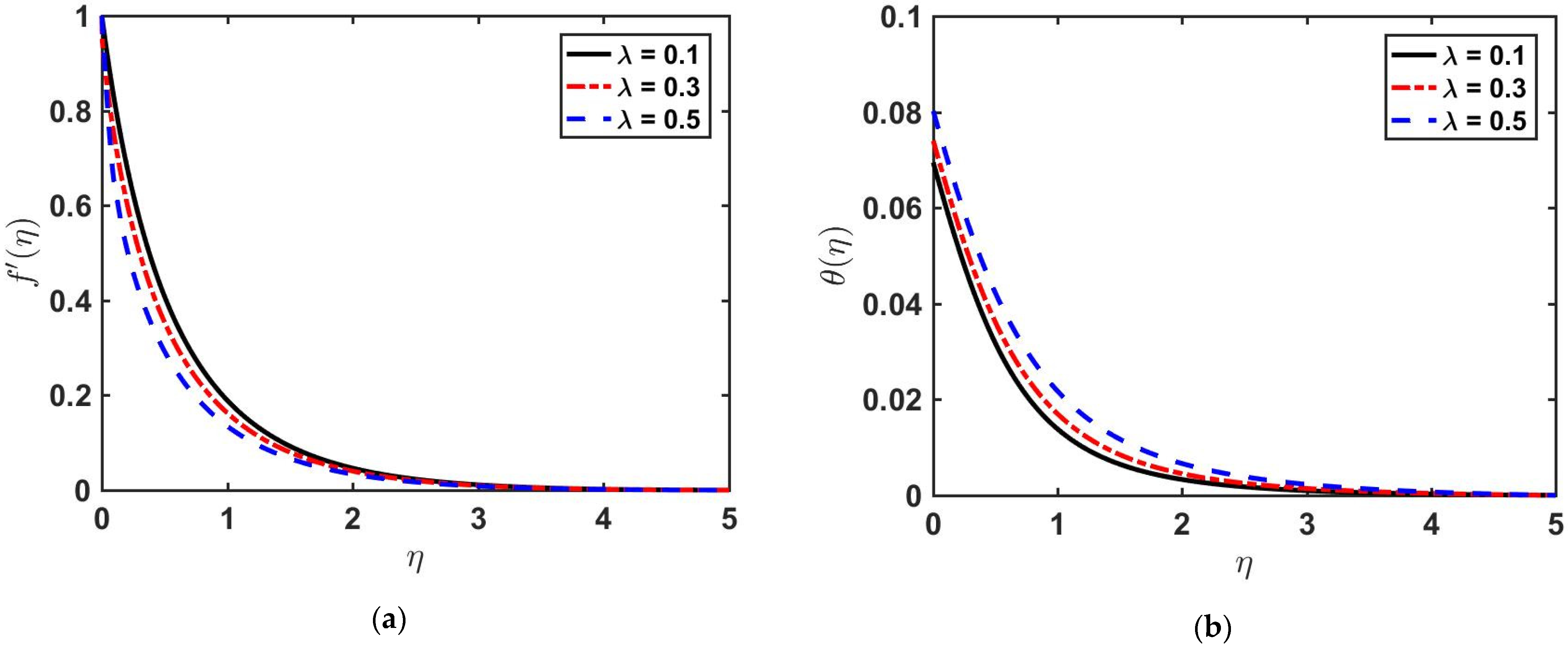
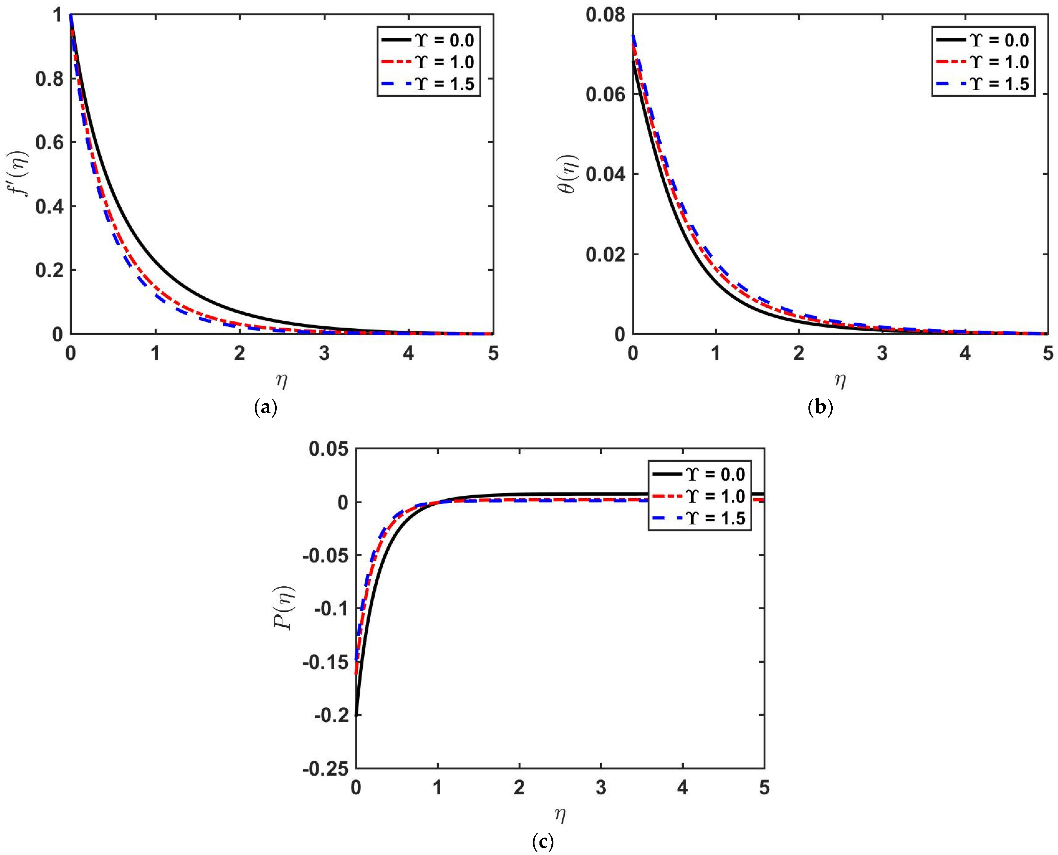
Figure 2a,b shows the impact of Williamson type fluid parameter
on the given velocity field
and temperature
profiles. The significant influence of the Williamson fluid parameter imparted on velocity is noted in
Figure 2a. It is noticed that for higher values of
, the value of
decreases, but
Figure 3 shows that the rising numbers the of Williamson type fluid parameter
yield an increase in the curve of the temperature
. Physically, we can say that the greater values of λ mean more and more sufficient relaxation times, offering more resistance to the fluid flow.
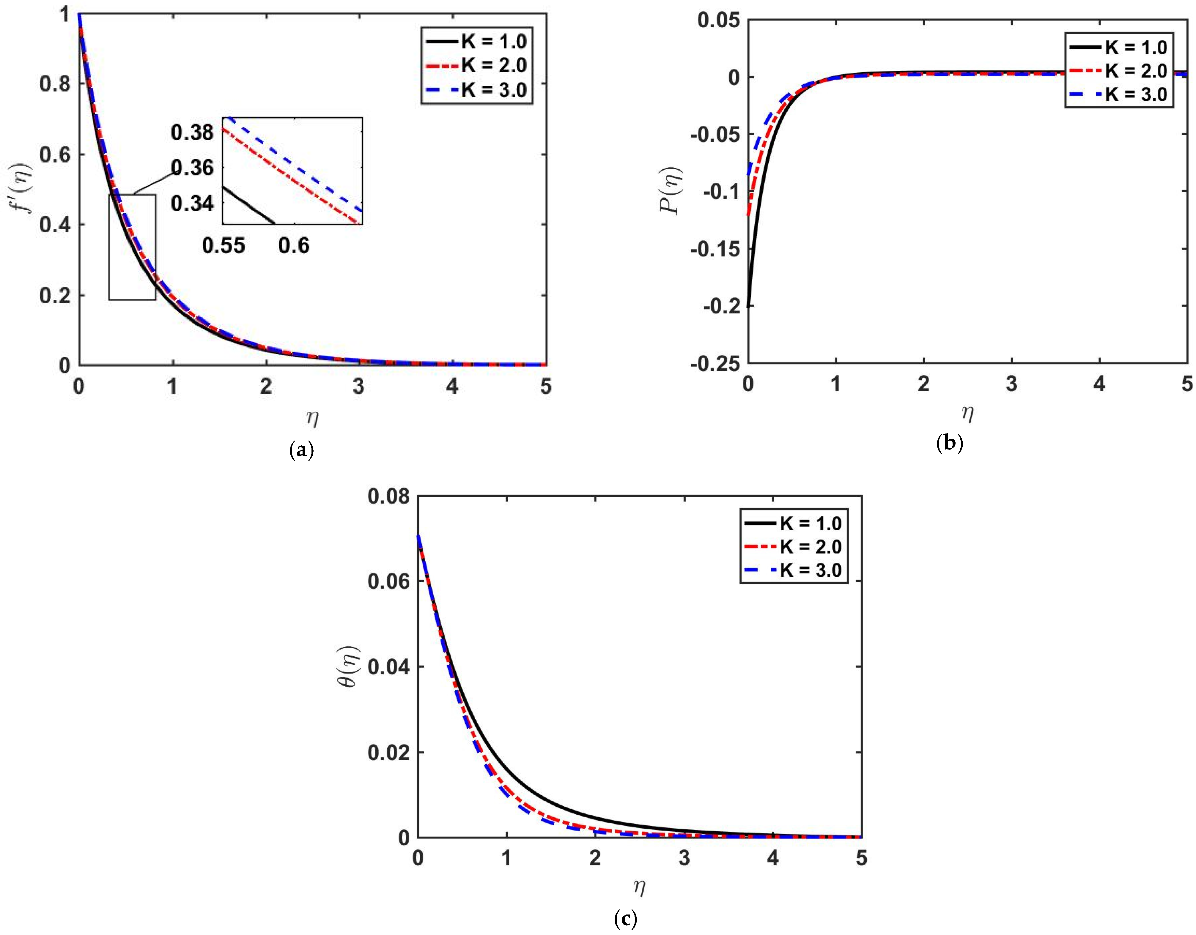
Figure 3a–c illustrate the effects of curvature
on
,
, and
. It is evident from
Figure 3a,b that the value of
and
increases with an enhancement in the value of the curvature parameter.
Figure 3c portrays the effect of curvature
on the distribution of heat
. By raising the value of the curvature factor, the graph shows a reduction in the value of heat distribution. As we increase
, the flatness of the stretching surface increases. Due to an increase in the flatness of the stretching surface, the flow velocity increases, and the temperature profile decreases because the resistance between the layers of the fluid reduces.
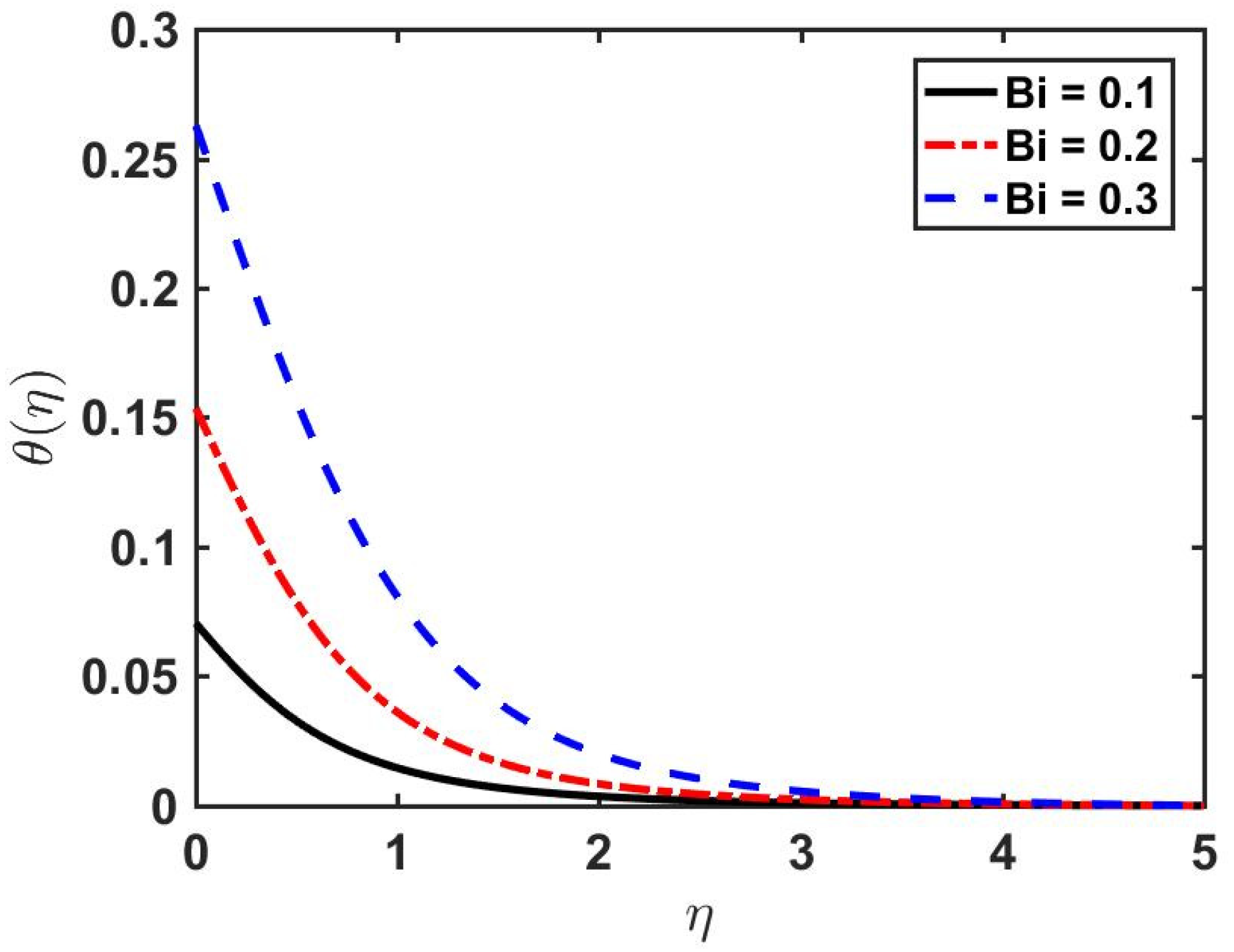
Figure 4 shows the impact of
on heat distribution. As we increase the value of the Biot number, there is a certain rise in the temperature profile because the Biot number is a relation within the internal conductive resistance to the surface offered convective resistance. It means that as we increase the Biot number, the internal conductive resistance increases, making the cross-boundary layer thickness stronger.
Figure 5 shows the impact of the Prandtl number given on the distribution of heat. We noticed from
Figure 5 that we see a decrease in heat distribution for the rising values of the Prandtl number. The Prandtl number
is the ratio between the momentum and thermal diffusivity. Therefore, the Prandtl factor owes an inverse relationship with thermal diffusivity. So, by increasing the Prandtl number, there is a decrement in heat distribution.
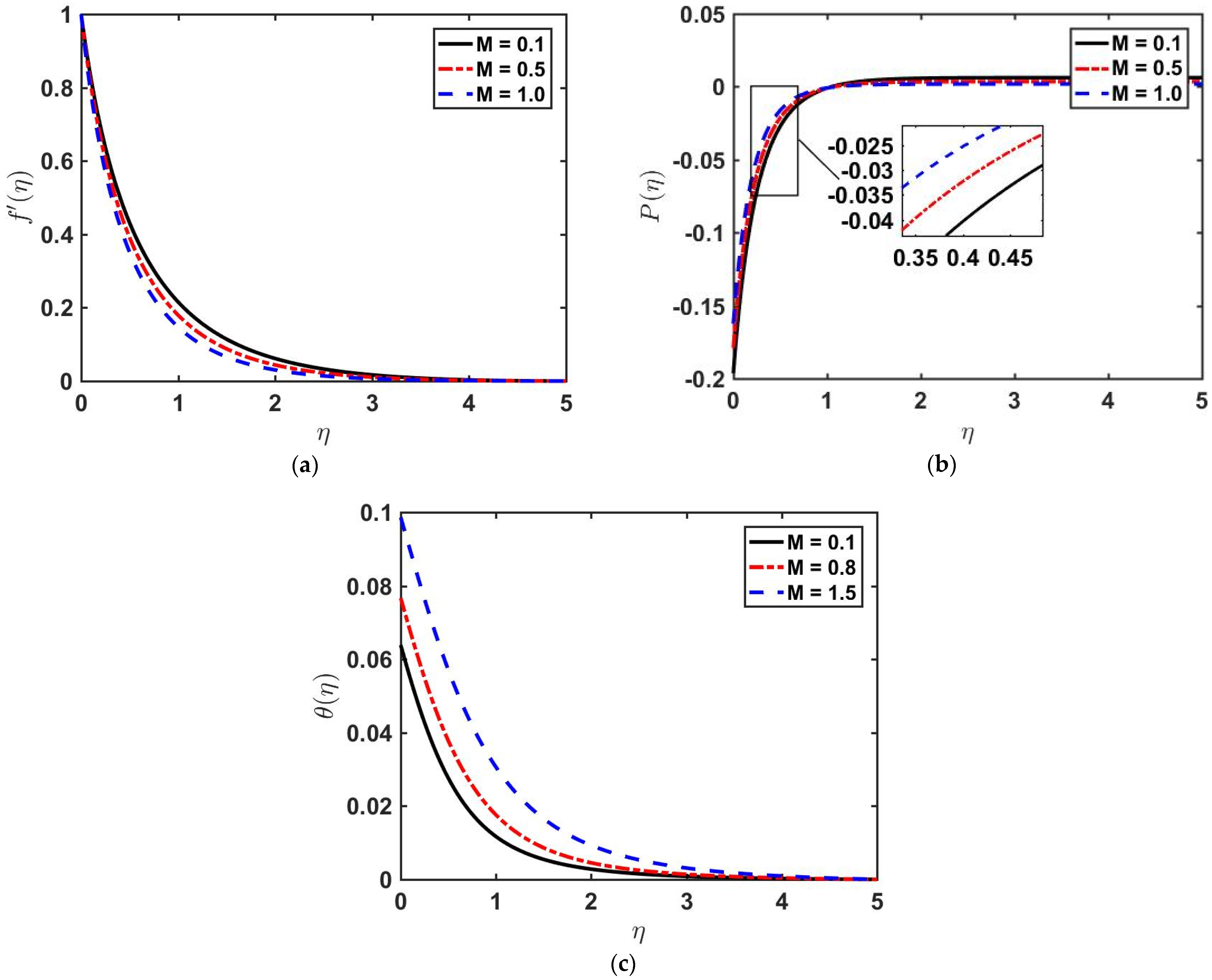
Figure 6a–c depicts the significant impact of magnetic field number
on velocity
, pressure
and temperature profile
.
Figure 6a shows that with the augment in cumulative magnetic number
, the velocity
depicts a reduction in values.
Figure 6b,c show that an opposite trend is noticed. The increase in
and temperature
result in an augmentation in the numerical values of
. This effect is seen due to increases in the Lorentz force. The Lorentz force acts perpendicular to the flow direction, which opposes velocity and increases pressure and temperature profiles.
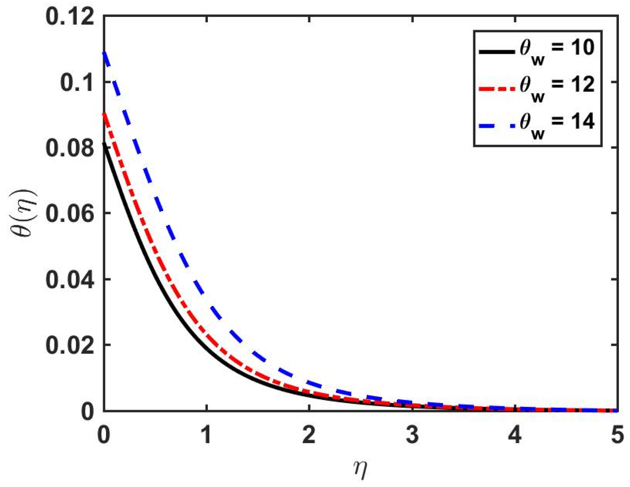
Figure 7 demonstrates the impact of
on the thermal profile. It is observed that when we raise
, the thermal profile also increases. Higher values of
means the temperature difference between
and
increases. This temperature difference causes an increase in the temperature profile.
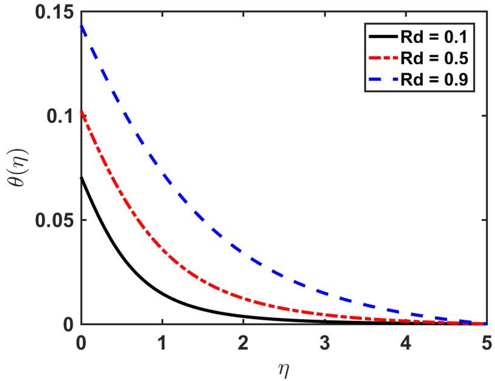
Figure 8 illustrates the effect of non-linear thermal radiation factor
on the thermal profile. It is noted that when we increase radiation parameter
, the temperature profile also augments. Since the stretching surface is heated, the energy emitted in the form of electromagnetic radiation causes an increase in the temperature profile.
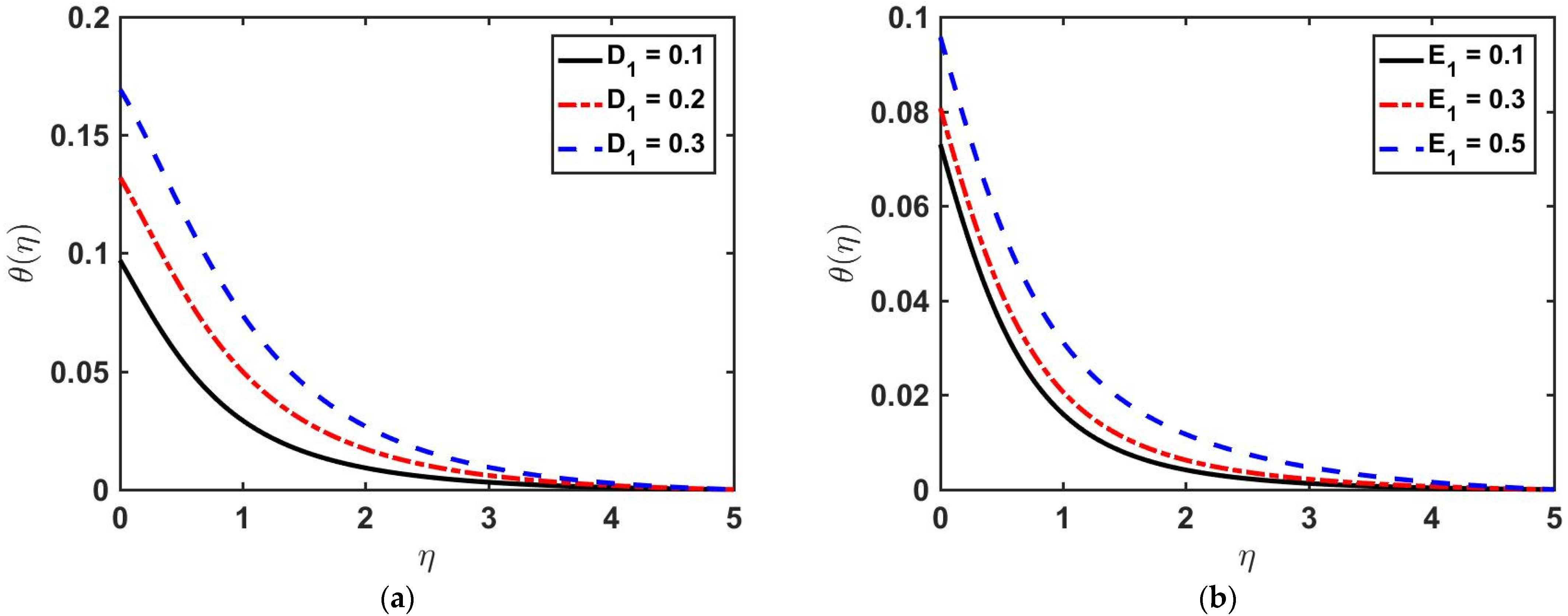
Figure 9a,b show the effect of irregular heat parameters on heat distribution. It is observed in both figures that by enhancing the values of
and
, there is a hike in the temperature distribution. By augmented values of irregular heat factors, the fluid temperature shows production results in the enhancement of the heat distribution of fluid.
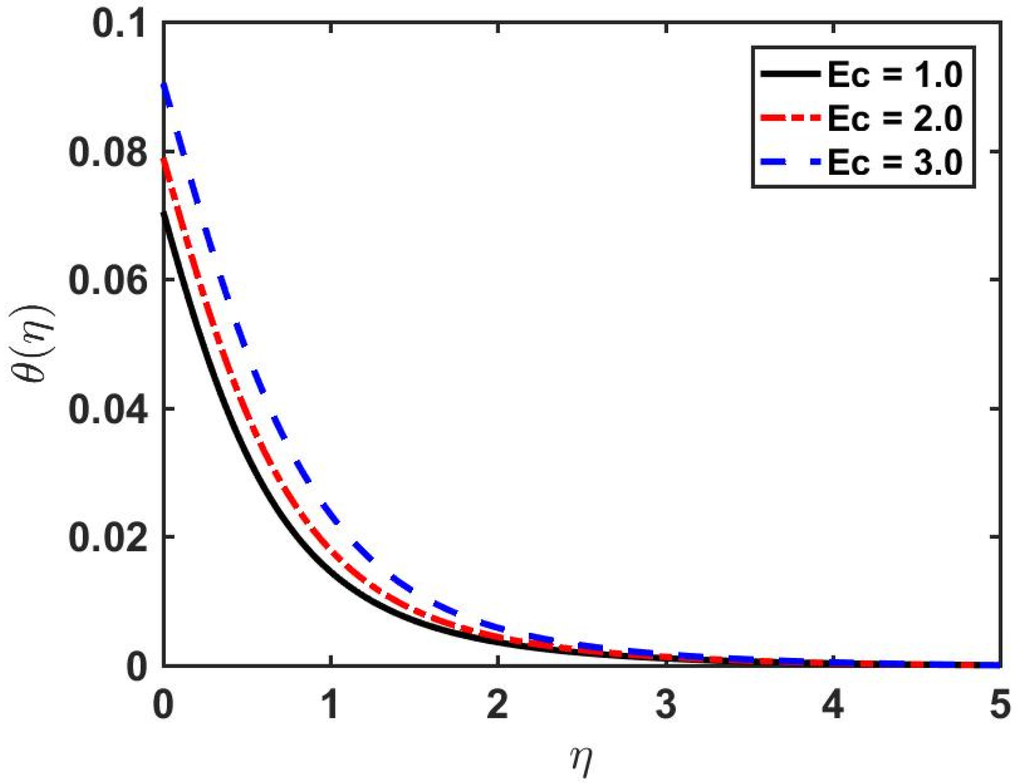
Figure 10 portrays the impact of the Eckert number on heat convection phenomena. It is observed from the graph that by increasing the Eckert number, there is an increase in heat distribution. The Eckert factor is defined as the ratio between the kinetic energy as well as the boundary layer enthalpy. So, by augmenting the value of the Eckert number, there is a rise in the heat distribution value.
Figure 11 shows the impact and significance of
on the temperature profile
. As we increase
the temperature profile also increases.
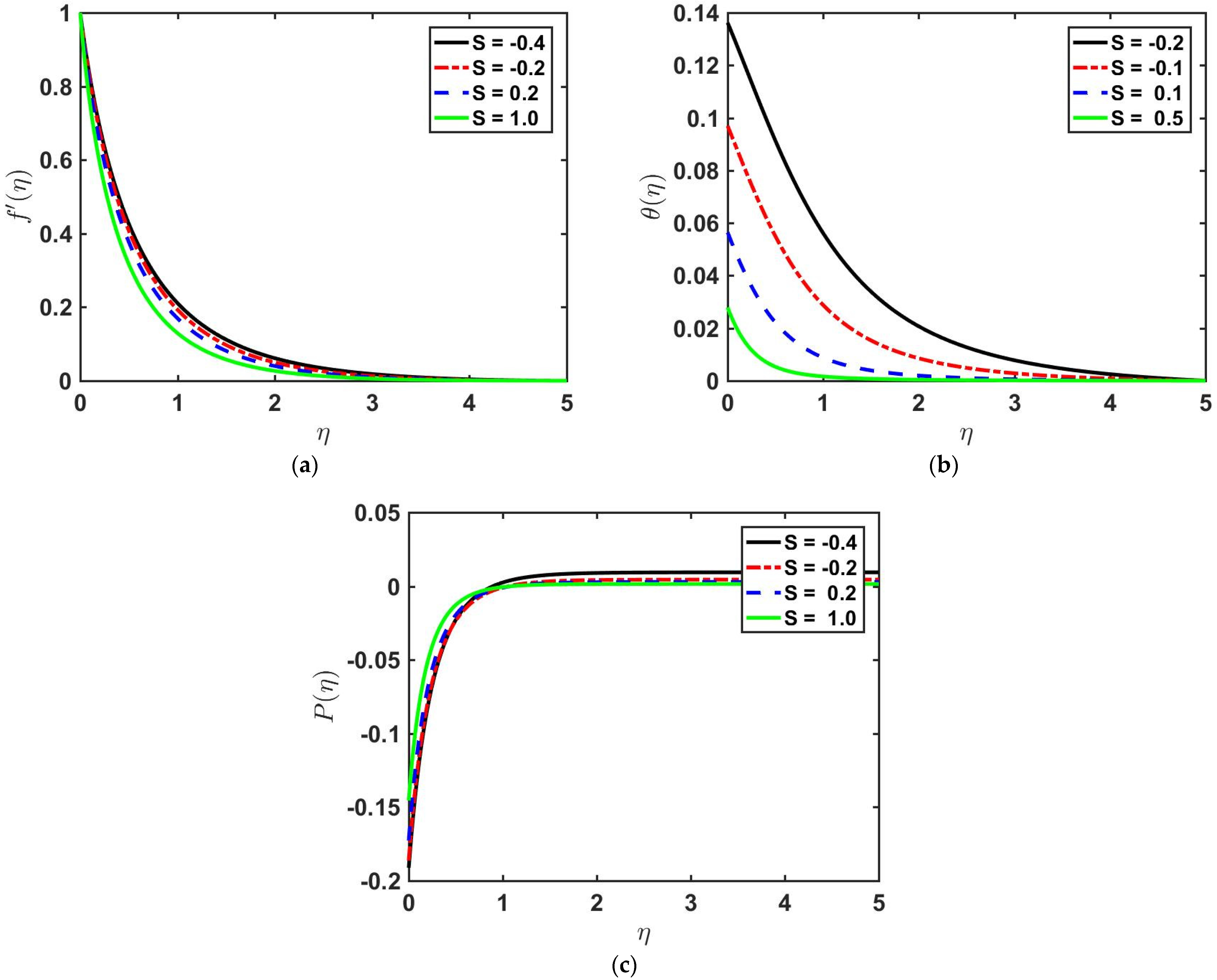
Figure 12a–c give us the effect of the suction/injection parameter
on the velocity field, temperature distribution, and pressure profile.
Figure 12a,b depict that as we increase the value of
, the velocity field, as well as temperature profile, declines. This effect is shown because by increasing the value of
, the suction/injection velocity increases, which is produced perpendicular to the direction of the flow, decreasing the motion of the fluid. The temperature profile decreases by increasing the value of
because the temperature near the surface is higher than the thermal state away from the surface by varying
; a reduction in temperature is shown in
Figure 12b.
Figure 12c depicts the pressure profile increasing as a result of the suction/injection factor on pressure from the interval (0,1); when the interval is (1,
), the pressure profile decreases. Mathematically this effect is shown due to the impact of velocity because the pressure is the function of the square of the velocity (see Equation (13)).
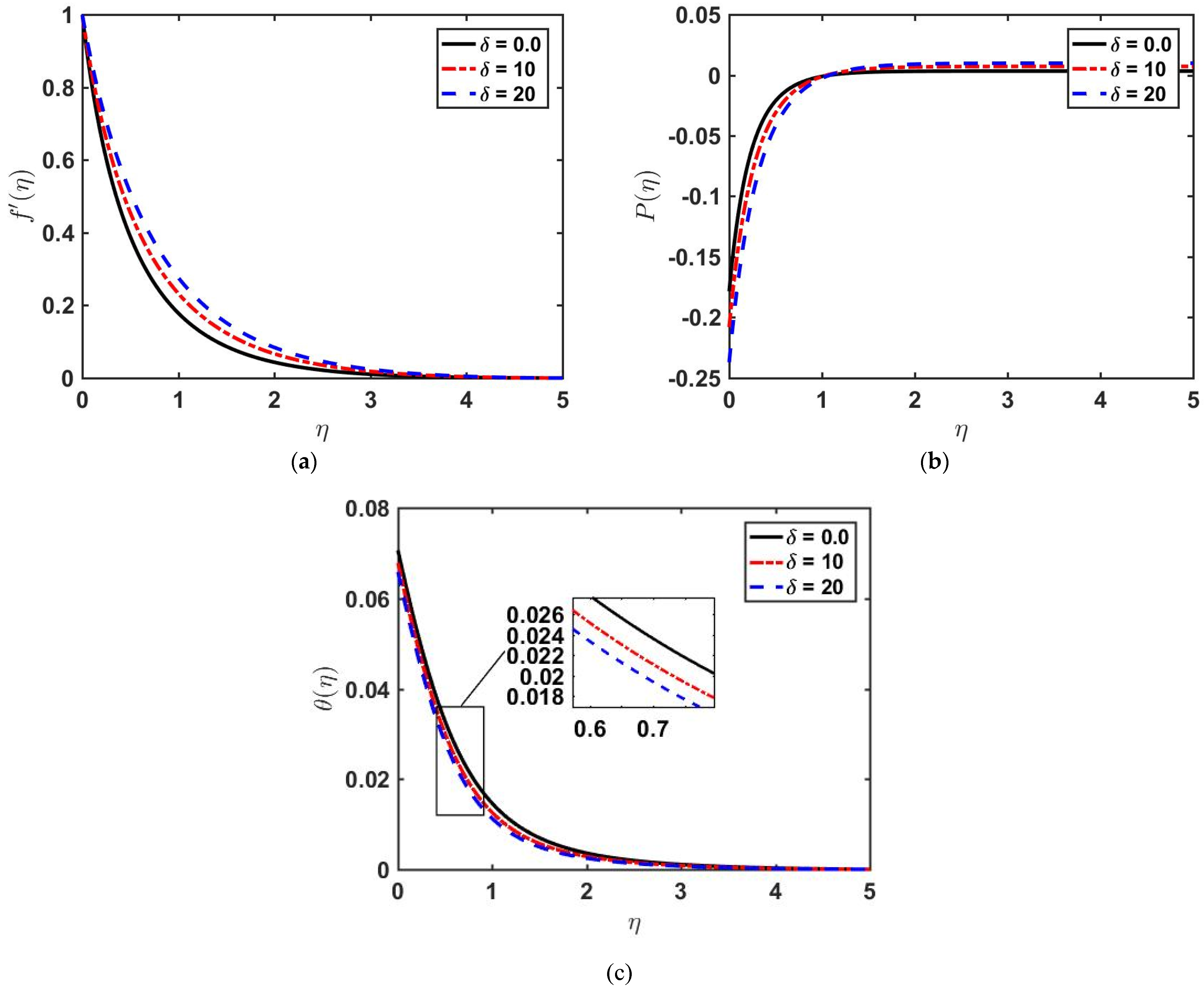
Figure 13a–c reveal the effects of the permeability factor on velocity, temperature, and pressure profiles. As we increase the permeability factor
, the velocity field decreases, and therefore, the temperature profile augments. The permeability factor
is dependent on a viscosity, which means that
increases the viscosity of the fluid under consideration, the flow of the velocity rate decreases, and the internal kinetic energy and heat transfer rates increase because of this effect.
Figure 13c depicts the effect of the permeability parameter on the pressure profile. The pressure profile increases from (0,1) and decreases from (1,5) for greater values of permeability parameter.
Figure 14a–c depict the significant impact of the buoyancy parameter
on the given velocity field, pressure profile, and thermal distribution. It is noticed from
Figure 14a that by raising the value of
, the velocity profile also categorically augments, whereas the temperature profile decreases (see
Figure 14c). From a physical point of view, the buoyancy force acts on the curved surface and stimulates the movement of the particle near the surface; due to this effect, the velocity field augments, and the thermal state declines. An interesting phenomenon is shown in
Figure 14b wherein a variation in
from (0,1) pressure profile decreases and increases from (1,5).


 ,
, 


