An Improved Conservative Direct Re-Initialization Method (ICDR) for Two-Phase Flow Simulations

Abstract

We introduce an improved conservative direct re-initialization (ICDR) method (for two-phase flow problems) as a new and efficient geometrical re-distancing scheme. The ICDR technique takes advantage of two mass-conserving and fast re-distancing schemes, as well as a global mass correction concept to reduce the extent of the mass loss/gain in two- and three-dimensional (2D and 3D) problems. We examine the ICDR method, at the first step, with two 2D benchmarks: the notched cylinder and the swirling flow vortex problems. To do so, we (for the first time) extensively analyze the dependency of the regenerated interface quality on both time-step and element sizes. Then, we quantitatively assess the results by employing a defined norm value, which evaluates the deviation from the exact solution. We also present a visual assessment by graphical demonstration of original and regenerated interfaces. In the next step, we investigate the performance of the ICDR in three-dimensional (3D) problems. For this purpose, we simulate drop deformation in a simple shear flow field. We describe our reason for this choice and show that, by employing the ICDR scheme, the results of our analysis comply with the existing numerical and experimental data in the literature.

1. Introduction

The level set (LS) method has been a popular and efficient means to capture interfaces in different two-phase (or multi-phase) flow fields since being introduced by Osher and Sethian [1]. In this method, the signed distance function (SDF) is approximated using the level set function or value ($\mathsf{\Phi }$). Therefore, one can employ the LS values at any arbitrary time ($t$) to explicitly estimate the interface without applying rigorous reconstruction algorithms, as is the case for the volume of fluid (VOF) method [2,3,4,5,6]. Besides, the evaluation of the interface normal vectors and curvature values are easily attainable, owing to the smoothness of the signed distance function [7].

The level set values equal the signed distance function at the initiation time ($t=0$) when the interface position is pre-defined. However, after some time steps ($\Delta t$) of the interface displacement, the LS function deviates from the SDF. Consequently, it is necessary to re-initialize the LS values to keep them as the signed distance function.

The re-initialization does not violate the overall mass conservation law since both phases’ mass summation is constant. However, due to the interface displacement after the re-initialization, the area or the volume occupied by one phase may reduce. On the contrary, the content of the other phase increases. The unphysical mass loss/gain after the re-initialization step is a numerical error.

Sussman et al. [8], for the first time, proposed a re-initialization method. They employed the Eikonal relation to force the Euclidean norm of the LS gradient to be one via solving a Hamilton–Jacobi (H-J) equation. Although their re-initialization strategy guarantees a finite thickness for the interface, it suffers from an unphysical mass loss/gain. Therefore, various methods have been proposed to compensate for this shortcoming. To mention a few, Hou introduced an area-preserving re-initialization, which involves solving a perturbed form of the H-J equation [9]. Moreover, Sussman et al. [10,11] improved the conservative properties of their re-initialization method by introducing a new term to the H-J equation. Yap et al. [12] employed the original H-J equation followed by a mass correction step based on a global mass conservation concept. Ville et al. [13] combined the level set and H-J equations to avoid a separate re-initialization step.

Olsen et al. [14,15] proposed the conservative level set method (CLS). They defined the level set values by a smoothed Heaviside function. Moreover, they employed the artificial compression method (ACM) [16]. They added a small diffusion term (artificial viscosity) to provide a mass-conservative re-initialization procedure, which evaluates a continuous interface with a constant thickness. Zhao et al. [17,18] then improved the CLS method (ICLS) by providing a more accurate estimation for the interface normal vectors and curvature values. Guermon et al. [19] extended the artificial compression and viscosity method to integrate the level set and the re-initialization equations. By employing their approach, one equation covers the interface advection and the re-initialization steps. Different techniques based on CLS are compared in [20] by Chiodi and Desjardins.

Besides the mentioned methods, which consist of solving a partial differential equation (PDE) as the re-initialization step, hybrid techniques are employed to improve the mass conservation. The particle level set (PLS) is a Lagrangian–Eulerian method which uses two groups of massless particles at two sides of the interface to update (re-initialize) the level set functions [21,22]. Sussman and Puckett [23] suggested another hybrid interface advection scheme which couples the LS and VOF methods (CLSVOF). Their technique employs the advantages of LS (explicit interface reconstruction) and VOF (mass conservation) methods.

Geometrical re-initialization is another approach to evaluate the SDF, which employs the spatial alignment of the interface to update the signed distance values. Therefore, one avoids the solution of a hyperbolic partial differential equation (e.g., the H-J equation). For example, a mass-conserving re-distancing scheme was proposed by Mut et al. [24] that employs unstructured triangular and tetrahedral meshes for two- and three-dimensional (2D and 3D) problems, respectively. Their technique, which we name the Mut method, comprises an iterative element-wise mass correction, followed by an averaging process between the nodes in a narrow band. Ausas et al. [25] employed the Mut method for a structured mesh and compared it with the H-J re-initialization. Cho et al. [26] and Ngo and Choi [27] introduced the direct re-distancing scheme, which provides a faster algorithm to evaluate each node’s distance function. We use the direct method to recall their algorithm.

This research introduces an improved conservative direct re-initialization (ICDR) method. The ICDR method is based on the Mut [24] approach. However, it comprises two improvements. Firstly it employs the direct method for a fast re-distancing [26,27]. Secondly, it considers a global mass correction [12] technique to reduce the extent of the mass loss/gain.

To provide a readable article, we have arranged the content of the manuscript as follows. The Section 2 describes the interface advection algorithm using the level set (LS) method. Section 3 provides a detailed description of the ICDR method and two other geometrical re-initialization techniques. In Section 4, we have quantitatively (by defining a norm value) and visually (by graphical demonstration) compared different geometrical re-initialization methods using a benchmark problem (the notched cylinder). Then, we have extensively studied the effect of time-step and mesh sizes on the accuracy of the ICDR method for two benchmark problems (the notched cylinder and swirling flow vortex). We have shown that the proposed method is applicable for both structured and unstructured meshes. In this section, we have also employed the ICDR method to study drop deformation in a simple shear flow field and have compared our results with the numerical and experimental data in the literature. Finally, in Section 5, the conclusion is provided.

2. Interface Advection Algorithm

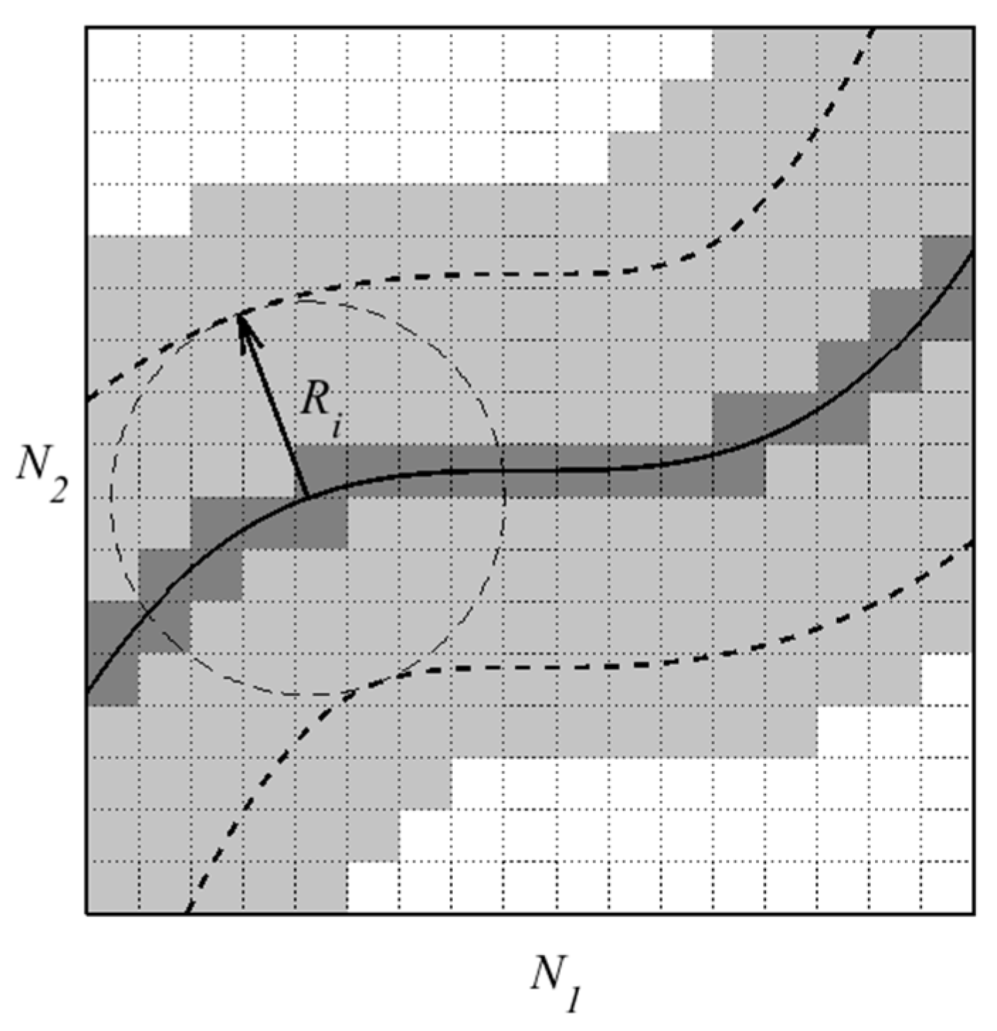
The level set function ($\mathsf{\Phi }$) in the LS method approximates the signed distance function. Therefore, a curved line or surface with the property of $\mathsf{\Phi }=0$ defines the interface. We arbitrarily assign the primary phase by $\mathsf{\Phi }>0$, and $\mathsf{\Phi }<0$ holds for the second phase. Since the LS values are essential in the vicinity of the interface, it is desired to employ a narrow-band LS method introduced by Chopp [28]. This technique limits the LS calculations to the interface vicinity instead of the whole domain. Figure 1, in a structured mesh $N_1\times N_2$, shows a typical interface (the solid line) and the elements in its vicinity. The elements in the vicinity of the interface are defined using the interface radius ($R_i$), which is twice or three times the greatest element diameter [7].

In Figure 1, the (light and dark) gray elements demonstrate the vicinity of the interface (the thick black line). Moreover, the dark gray shows active elements of the grids, which contain an interface. Here, we normalize the signed distance function as stated in Equation (1), and name it nodal volume fraction.

$$f=\{\begin{array}{cc}1& d\ge R_i\\ \frac{1}{2}+\frac{d}{R_i}& -R_i<d<R_i\\ 0& d\le -R_i\end{array}$$

(1)

In Equation (1), the parameters $d$ and $f$ show the signed distance function and the nodal volume fraction, respectively. On this basis, the interface advection equation would be as follows:

$$\frac{\partial f}{\partial t}+u_i\frac{\partial f}{\partial x_i}=0$$

(2)

In Equation (2), which is based on Einstein summation notations over a common index, $u_i \left(i=1, 2, \mathrm{and} 3\right)$ are the components of the velocity vector ($\overrightarrow{\mathit{u}}=\left(u_1,u_2,u_3\right)$). The parameter $x_i \left(i=1, 2, \mathrm{and} 3\right)$ show the coordinates of any arbitrary point in a Cartesian reference frame.

Several stable strategies to solve the interface advection equation are proposed in the literature: Streamline Upwind Petrov–Galerkin [24] and Taylor–Galerkin [26] methods. In this research, we have employed a least-squares finite element method [7,27]. For this purpose, the domain is divided into rectangular or hexahedral subdomains or elements for 2D and 3D cases, respectively. Then, a linear-based shape function ($\varphi$) is considered to evaluate the volume fraction ($f$) in each element. Therefore, Equation (2) is discretized as follows:

$$\langle \varphi \rangle \frac{\partial \left\{f\right\}}{\partial t}+u_i\frac{\partial \langle \varphi \rangle }{\partial x_i}\left\{f\right\}=0$$

(3)

where $\left\{f\right\}$ and $\langle \varphi \rangle$ are the column-wise and row-wise vectors of the calculated volume fractions and shape function coefficients in each element, respectively. To solve Equation (3), the explicit values of the velocity components ($u_i$) from the current time step are used. Additionally, the Crank–Nicolson method is employed to evaluate the nodal values of the volume fraction, as stated in Equation (4).

$$f=\alpha f^{\left(1\right)}+\left(1-\alpha \right)f^{\left(0\right)}$$

(4)

In this equation, the parameters $f^{\left(0\right)}$ and $f^{\left(1\right)}$ are the nodal volume fraction values at the current and next steps, respectively. The term $\alpha$ is the Crank–Nicolson adjusting parameters and changes between 0 and 1. $\alpha =1$ and $\alpha =0$ turn the equation to fully implicit and explicit methods, correspondingly. Substituting the $f$ from Equation (4) into Equation (3) results in Equation (5a–c)

$$\langle {\mathsf{\Phi }}_1\rangle \left\{f^{\left(1\right)}\right\}=\langle {\mathsf{\Phi }}_2\rangle \left\{f^{\left(0\right)}\right\}$$

(5a)

$$\langle {\mathsf{\Phi }}_1\rangle =\langle \varphi \rangle +\alpha u_i\Delta t\frac{\partial \langle \varphi \rangle }{\partial x_i}$$

(5b)

$$\langle {\mathsf{\Phi }}_2\rangle =\langle \varphi \rangle -\left(1-\alpha \right)u_i\Delta t\frac{\partial \langle \varphi \rangle }{\partial x_i}$$

(5c)

The parameter $\Delta t$ in Equation (5b,c) is the time-step size. The weighted residual form of Equation (5a) is:

$$\left[{{\displaystyle \int }}_{\Omega }^{}\left\{\omega \right\}\langle {\mathsf{\Phi }}_1\rangle d\Omega \right]\left\{f^{\left(1\right)}\right\}=\left\{{{\displaystyle \int }}_{\Omega }^{}\left\{\omega \right\}\langle {\mathsf{\Phi }}_2\rangle \left\{f^{\left(0\right)}\right\}d\Omega \right\}$$

(6)

In Equation (6), $\omega$ is the weight function, which is equal to ${\mathsf{\Phi }}_1$ in our least-square finite element method [29]. Equation (6) results in a linear set of equations for a known velocity field.

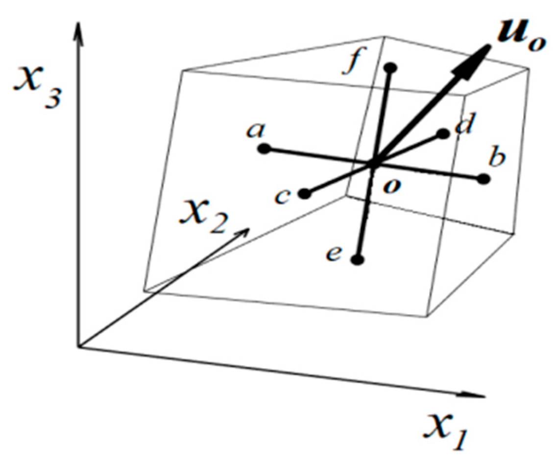
The time step ($\Delta t$) is an essential parameter in the solution of Equation (6). To find a suitable time increment, we define a characteristic time for each element. For this purpose, we assume an arbitrary 3D element, as shown in Figure 2. In this element, three different vectors $\overrightarrow{ab}$, $\overrightarrow{cd}$ and $\overrightarrow{ef}$ can easily be defined by connecting the middle of the front faces. If the velocity at the center of the element is $\overrightarrow{{\mathit{u}}_o}=\left(u_{o1},u_{o2},u_{o3}\right)$, the projection of the velocity vector on each vector would be:

$$u_{ab}=\overrightarrow{{\mathit{u}}_o}· \overrightarrow{ab}$$

(7a)

$$u_{cd}=\overrightarrow{{\mathit{u}}_o}· \overrightarrow{cd}$$

(7b)

$$u_{ef}=\overrightarrow{{\mathit{u}}_o}· \overrightarrow{ef}$$

(7c)

In Equation (7a,b), the operator “.” demonstrates the dot product of the vectors. Then, the element characteristic time ($\Delta t^{*}$) is defined as stated in Equation (8a–c).

$$\Delta t_1=\frac{\overrightarrow{\Vert ab\Vert }}{\left|u_{ab}\right|}$$

(8a)

$$\Delta t_2=\frac{\overrightarrow{\Vert cd\Vert }}{\left|u_{cd}\right|}$$

(8b)

$$\Delta t_3=\frac{\overrightarrow{\Vert ef\Vert }}{\left|u_{ef}\right|}$$

(8c)

$$\Delta t^{*}=min\left(\Delta t_1,\Delta t_2,\Delta t_3\right)$$

(8d)

In Equation (8a,b), the operators $\Vert \Vert$ and $| |$ stand for the Euclidean size of a vector and the absolute value of a scalar quantity, respectively. Moreover, the operator $min$ shows the minimum amount. Similarly, we evaluate the characteristic time in a 2D element.

Mathematically, there are no limitations for the time step, when an implicit solution is used ($\alpha =1$). Moreover, the limitation $\Delta t\le min\left(\Delta t_i^{*}\right)$ (i: the number of the active elements) must be considered for an explicit solution ($\alpha =0$). In our Crank-Nickelson scheme, we have set $\alpha =1/2$ (as selected in [24]), because it can provide more acceptable results based on our numerical experiments. In this case, the limitation for time step would be as follows:

$$\Delta t\le 2min\left(\Delta t_i^{*}\right)$$

(9)

From now on, we briefly use $\Delta t^{*}$ instead of $min\left(\Delta t_i^{*}\right)$, and name it the characteristic time of the two-phase flow domain

After solving Equation (5a) for each time step, we can easily reconstruct the interface. For this purpose, we look for the active elements or the subdomains, which contain at least one node with $f>1/2$ and another node with $f<1/2$. If $f_1>1/2$ and $f_2<1/2$ are the volume fractions of nodes 1 and 2 on an element edge, we can find the interface intersection point by a simple linear interpolation, as stated in Equation (10).

$${\overrightarrow{\mathit{x}}}_{\mathit{i}\mathit{n}\mathit{t}}=\frac{{\overrightarrow{\mathit{x}}}_{\mathit{2}}-{\overrightarrow{\mathit{x}}}_{\mathit{1}}}{f_2-f_1}\left(\frac{1}{2}-f_1\right)+{\overrightarrow{\mathit{x}}}_{\mathit{1}}$$

(10)

In Equation (10), ${\overrightarrow{\mathit{x}}}_{\mathit{i}\mathit{n}\mathit{t}}$, ${\overrightarrow{\mathit{x}}}_{\mathit{1}}$, and ${\overrightarrow{\mathit{x}}}_{\mathit{2}}$ are the spatial coordinates of the intersection point, the first node, and the second node, respectively.

3. Geometrical Re-Initialization

The solution of Equation (5a), using any stabilized finite element, finite volume, or finite difference, introduces an artificial diffusion to the problem. Therefore, it is expectable that the level set function ($\mathsf{\Phi }$) deviates from the signed distance function. Although employing a narrow-band technique, such as the local least-square finite element method (LLSFEM) [7], prevents the excessive interface diffusion, it does not remove the demand for the re-initialization step.

Different types of re-distancing or re-initialization are discussed in the introduction section. However, in this research, we concentrate on the geometrical re-initialization.

3.1. The Motivations and Preliminaries

The geometrical re-initialization comprises the methods which calculate the nodal distance function (DF) using the spatial coordinates of the nodes and the interface. The sign of the DF is determined by the sign of the nodal level set values.

By introducing a finite number of imaginary particles on the interface and searching for the shortest distance between each node and the particles, one can simply evaluate the DF ($\left|d\right|$). The particle-based method is a time-consuming task. However, it could be more efficient by limiting the search algorithm to the narrow band’s nodes (e.g., Figure 1).

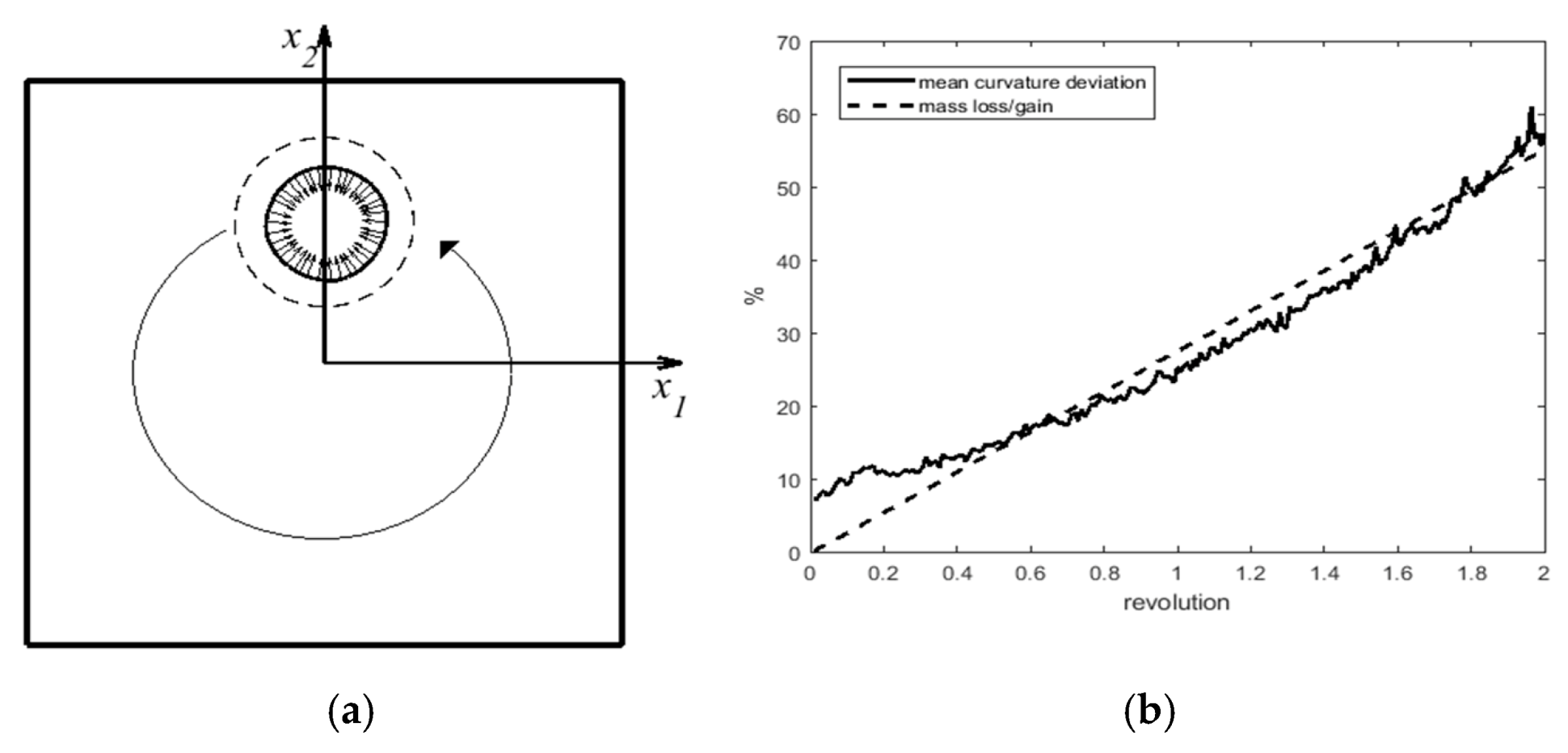
Taking the particle-based scheme to re-initialize the level set values will lead to a severe mass loss/gain, which is attributed to the interface displacement after re-initialization. To illustrate the movement of the interface, we provide an example. The problem consists of a circle with an arbitrary radius (e.g., $R_{circle}=0.15)$ in a square ($1\times 1$) flow domain. The spatial position of the circle center is ${\overrightarrow{\mathit{x}}}_{circle}=\left(0,0.25\right)$ as shown in Figure 3a, and a 2D solid-rotational flow around ${\overrightarrow{\mathit{x}}}_O=\left(0,0\right)$ is considered ($\overrightarrow{\mathit{u}}=\left(\frac{-\pi }{314}{x}_2,\frac{\pi }{314}{x}_1\right)$). The circle rotates two revolutions around ${\overrightarrow{\mathit{x}}}_O=\left(0,0\right)$ in a structured $50\times 50$ mesh.

Figure 3a shows that the reconstructed circle after two revolutions (solid line) is considerably smaller than the original one (dashed line), which is due to the mass loss in the circle. The dashed line in Figure 3b quantifies the extent of the mass loss during the revolutions. The solid line in Figure 3b shows the mean deviation of the active element curvature ($\kappa$) from the original one ($1/R_{circle}$), which is mainly attributed to the mass loss and the change of the circle radius. The curvature ($\kappa$) and normal vector ($\overrightarrow{\mathit{n}}$) in each active element are easily calculated using Equation (11a,b). In these equations, the symbols $\mathbf{\nabla }$ and $\mathbf{\nabla }$ are the gradient and divergence operators, respectively.

$$\overrightarrow{\mathit{n}}=\frac{\mathbf{\nabla }\phi }{\Vert \mathbf{\nabla }\phi \Vert }=\frac{\mathbf{\nabla }f}{\Vert \mathbf{\nabla }f\Vert }$$

(11a)

$$\kappa =\mathbf{\nabla }·\overrightarrow{\mathit{n}}$$

(11b)

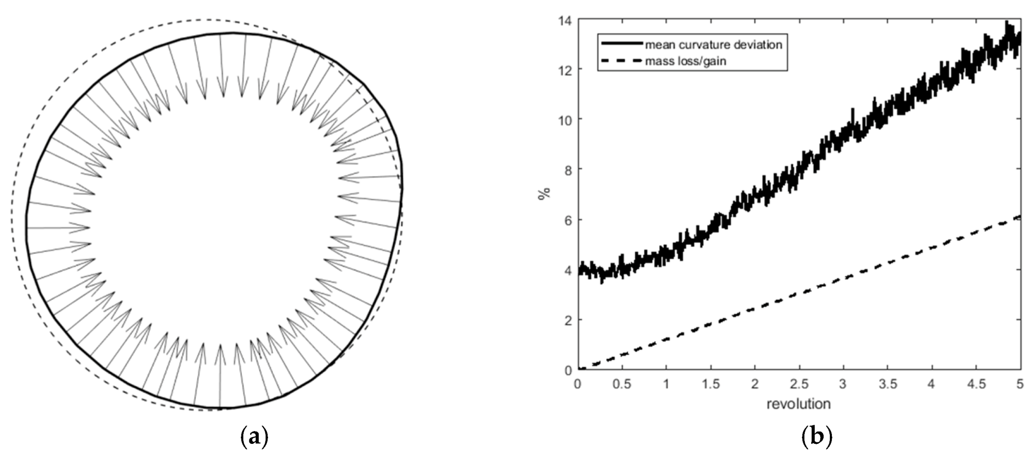
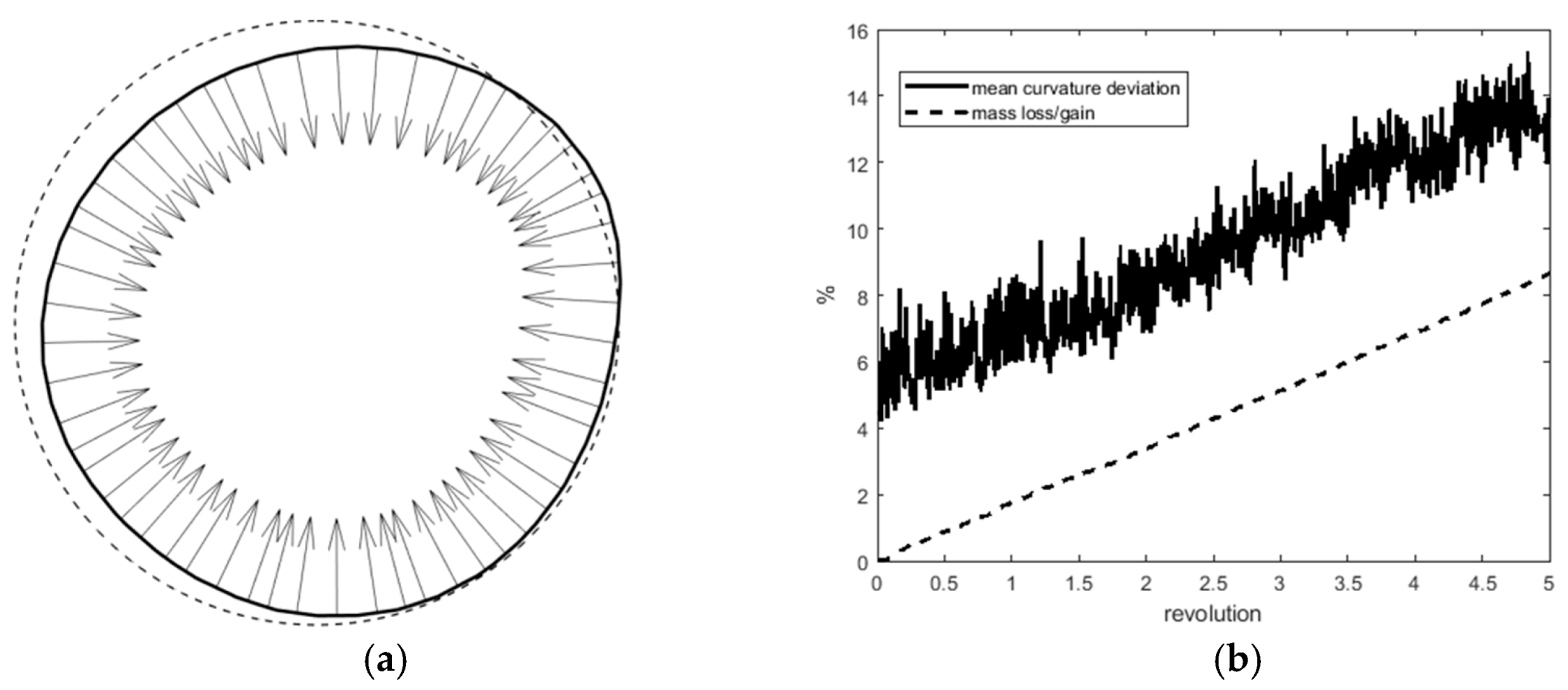
A direct re-initialization method is another approach which is proposed by Cho et al. [26] and Ngo and Choi [27]. In their scheme (the direct method), the DF is the shortest perpendicular distance up to the interface segments. If the perpendiculars’ foot is not inside the interface segments, the DF would be the minimum distance of each node up to the interface/element intersections. The direct method estimates the distance function equal to the particle-based scheme. Nevertheless, it requires a shorter computing time because it limits the number of searches to find the minimum distance. This method excludes the nodes of active elements from the re-initialization (the nodes in the dark-grey area of Figure 1) to avoid the displacement of the interface. Therefore, the direct approach shows good mass-conservative properties, although it does not take any measure for mass correction. To investigate this problem, in Figure 4a, we can compare the reconstructed circle (solid line) after five revolutions with the original circle (dashed line). The extent of the mass loss and the mean curvature deviation, as shown respectively by the dashed and solid lines in Figure 4b, are smaller than their corresponding values in Figure 3b.

The solid line in Figure 4b shows an increasing trend for the deviation of the curvature values, which are calculated using Equation (11a,b). These equations employ the nodal volume fractions (or the LS values) on each active element and its neighbor elements to evaluate the value of $\mathbf{\nabla }f$ [7] on the nodes. When the nodes of active grids do not participate in the re-distancing procedure, inaccurate estimation of $\mathbf{\nabla }f$ and $\kappa$ are expected, due to unsmooth values of $f$.

Mut et al. [24] introduced a two-step method for estimation of the DF, which comprises initialization and evaluation stages. The initialization step calculates each node’s distance function. As described for the particle-based scheme, this step consists of a considerable mass loss/gain due to the interface displacement. Therefore, during the evaluation step, the distance function values are corrected. Mut et al. developed the method for triangular and tetrahedral grids, and we have adapted it to rectangular and hexagonal meshes.

Any interface displacement after the re-initialization step leads to an unwanted variation of the area ($\Delta A$) occupied by the primary phase in each active element. Equation (12a–c) evaluate the mass change in an active element (e.g., element number $i$). In these equations, the superscripts 0 and 1 stand for the values before and after re-initialization, respectively. Moreover, the operator $\lfloor \rfloor$ calculates the integer part of a real number and ${\mathsf{\Omega }}_{\mathrm{e}}$ depicts the element domain. The symbol $A$ is a function that calculates the area (or volume) of the primary phase in an element with nodal volume factions of $\left\{f\right\}$.

$$\Delta A_i=A\left(\left\{f_i^0\right\}\right)-A\left(\left\{f_i^1\right\}\right)$$

(12a)

$$A\left(\left\{f_i^0\right\}\right)={{\displaystyle \int }}_{{\mathsf{\Omega }}_e}^{}\lfloor \langle \varphi \rangle \left\{f_i^0\right\}+\frac{1}{2}\rfloor d{x}_{1}d{x}_2$$

(12b)

$$A\left(\left\{f_i^1\right\}\right)={{\displaystyle \int }}_{{\mathsf{\Omega }}_e}^{}\lfloor \langle \varphi \rangle \left\{f_i^1\right\}+\frac{1}{2}\rfloor d{x}_{1}d{x}_2$$

(12c)

To our knowledge, the values of $\Delta A_i$ are non-zero just for the active elements. To compensate for the area changes, Mut et al. [24] suggested a mass correction value (${\delta }_i$) for each active element, which is the root of the area residual ($\mathcal{R}$), as defined in Equation (13):

$$\mathcal{R}\left({\delta }_i\right)=A\left(\left\{f_i^0\right\}\right)-A\left(\left\{f_i^1\right\}+{\delta }_i\right)=0$$

(13)

They solved Equation (13) for each active element by employing the scant method, as summarized in Equation (14):

$${\delta }_i^{\left(m+2\right)}={\delta }_i^{\left(m+1\right)}-\mathcal{R}\left({\delta }_i^{\left(m+1\right)}\right)\frac{{\delta }_i^{\left(m+1\right)}-{\delta }_i^{\left(m\right)}}{\mathcal{R}\left({\delta }_i^{\left(m+1\right)}\right)-\mathcal{R}\left({\delta }_i^{\left(m\right)}\right)}$$

(14)

In Equation (14), the superscripts $\left(m\right)$ to $\left(m+2\right)$ denote the iteration steps. This equation converges after 2 or 3 iterations (${\delta }_i^{\left(m+1\right)}-{\delta }_i^{\left(m\right)}<0.5\times {10}^{-4}$). The value of ${\delta }_i$ is attributed to the nodes of the $i^{th}$ element, which is zero for any non-active element. By averaging ${\delta }_i$ values of active elements that share a node, the nodal mass correction values (${\delta }^{*}$) are evaluated. For example, if node $j$ is attached to two active elements $i_1$ and $i_2$, ${\delta }_j^{*}$ would be as follows:

$${\delta }_j^{*}=\frac{{\delta }_{i_1}+{\delta }_{i_2}}{2}$$

(15)

Then, the corrected volume fraction values ($f^{*}$) are evaluated using Equation (16):

$$f^{*}=f^1+\beta {\delta }^{*}$$

(16)

In Equation (16), the $\beta$ parameter is a scalar quantity, adjusted using a mass conservation criterion. Mut et al. [24] calculated $\beta$ by considering Equation (17), which keeps the main phase area (or volume) unchanged, all over the elements ($N$), before and after re-initialization.

$$\sum _{i=1}^N{{\displaystyle \int }}_{{\mathsf{\Omega }}_e}^{}\lfloor \langle \varphi \rangle \left\{f_i^{*}\right\}+\frac{1}{2}\rfloor d{x}_{1}d{x}_2=\sum _{i=1}^N{{\displaystyle \int }}_{{\mathsf{\Omega }}_e}^{}\lfloor \langle \varphi \rangle \left\{f_i^0\right\}+\frac{1}{2}\rfloor d{x}_{1}d{x}_2$$

(17)

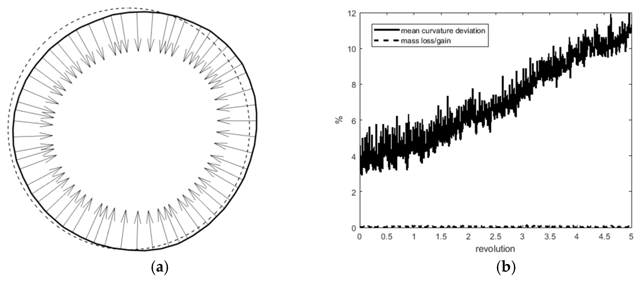
Figure 5 presents the results of the solid circle revolution, employing Equations (12)–(17). Comparing the solid line (the circle after five revolutions) and the original circle (dashed line) in Figure 5a reveals the circle deformation in a solid rotational flow field. The mass loss shown in Figure 5b by the dashed line does not suggest any improvement compared to the direct re-initialization method (Figure 4b). We attribute this to the concept of Equation (17), in which the mass correction is not performed according to the content of the primary phase at the onset of the problem.

3.2. Improved Conservative Direct Re-Initialization (ICDR)

In this section, we introduce the improved conservative direct re-initialization (ICDR) method. This approach employs the direct technique [26,27], which is faster than the particle-based scheme, to find the nodal distance function (DF). To reduce the mass loss/gain, we take the Mut strategy [24] and modify it using a global mass conservation concept [12]. The ICDR method, adapted to rectangular and hexagonal elements, involves four steps, as follows:

Step 1: We evaluate the nodal distance functions of the active elements (e.g., just the nodes in the dark gray section of Figure 1) using the direct technique.

Step 2: By employing the nodal values of the volume fraction before and after re-distancing, we calculate the mass correction value of the node (${\delta }^{*}$), according to Equations (12)–(15).

Step 3: We replace Equation (17) with Equation (18), which guarantees global mass conservation for each phase. Equation (18) forces the content of the primary phase to be initial value (i.e., $t=0$) plus the part, which is lost or gained during the re-initialization step ($\sum _{i=1}^N\Delta A_i$).

$$\begin{array}{c}{\displaystyle \sum _{i=1}^N}{{\displaystyle \int }}_{{\mathsf{\Omega }}_e}^{}\lfloor \langle \varphi \rangle \left\{f_i^{*}\right\}+\frac{1}{2}\rfloor d{x}_{1}d{x}_2=\\ {\displaystyle \sum _{i=1}^N}{{\displaystyle \int }}_{{\mathsf{\Omega }}_e}^{}\lfloor \langle \varphi \rangle \left\{f_{i,t=0}\right\}+\frac{1}{2}\rfloor d{x}_{1}d{x}_2+{\displaystyle \sum _{i=1}^N}\Delta A_i\end{array}$$

(18)

Step 4: To obtain a smoothed set of values for the SD or nodal volume fraction, we re-distance the nodes in the vicinity of the interface (e.g., the dark and light gray in Figure 1) using the direct method.

By modifying the mass correction criterion in the third step, we anticipate better mass conservation properties for the ICDR method. Moreover, with a final re-initialization at step (4), a smoother set of nodal volume fraction and a better approximation for curvature values is expectable. These two steps distinguish the ICDR method from the existing geometrical re-initialization methods. To investigate the expected improvements, we compare the results for the rotating circle’s problem using the ICDR in Figure 6a,b with the corresponding results in Figure 4 and Figure 5.

The circle deformation after five revolutions in Figure 6a seems to be less in comparison to Figure 4a and Figure 5a. Moreover, the dashed line in Figure 6b demonstrates the superior conservative properties of the ICDR method in comparison to two other methods, as shown in Figure 4b and Figure 5b. Similarly, the deviation of the mean curvature values from its exact value ($\kappa =1/R_{circle}=$4) is less for the ICDR method (the solid lines in Figure 4b, Figure 5b, and Figure 6b).

4. Results and Discussion

In this section, we examine the viability of the ICDR method. For this purpose, we use two benchmark problems to study the interface reconstruction and mass-conservative properties in two-dimensional form. We show that the new re-initialization algorithm is applicable for structured and unstructured meshes. Finally, we use the ICDR method for three-dimensional drop deformation problems.

4.1. Comparison of the Geometrical Re-Initialization Methods in 2D

To compare different re-initialization strategies, we use the notched cylinder problem, which was initially introduced by Zalesak [30]. In this problem, a notched cylinder with pre-defined dimensions revolves in a solid-rotational flow field, as introduced in Section 3.1. We expect the notched cylinder to comply with its original shape after each revolution. However, there exists some deviation when using any advection and re-initialization method. A defined norm value of ${ϵ}_1$ in Equation (19) is the criteria for quantifying the mentioned deviation. In Equation (19), the interface length is shown by $L_{int}$.

$${ϵ}_1=\frac{1}{L_{int}}\sum _{i=1}^N\left|A\left(\left\{f_{i,t=0}\right\}\right)-A\left(\left\{f_i\right\}\right)\right|$$

(19)

To have a comparison with the literature, we choose the domain with $N_1\times N_2=200\times 200$ rectangular elements, which is the closest one to the cases with 80,000 and 79,668 triangular elements in [24,27], respectively. Besides the time step $\Delta t=0.5$, we have considered $\Delta t=1.0$ to compare the effect of time steps in different methods. Notably, all of the results are generated using rectangular sub-domains or elements.

Figure 7a,b show the rotated cylinder after the first and fifth revolutions, respectively. In these figures, the dotted and solid lines show the results for $\Delta t=1.0$ and $\Delta t=0.5$, correspondingly. As depicted in Figure 7a, the direct method after the first revolution shows some unevenness at the lower part of the notched cylinder. The jagged area, which is similarly reported in Figure 8 of [27], expands during the second to fifth revolutions, as shown in Figure 7b. We attribute this to the nodes of the active elements, which are not re-initialized. We do not expect such deviations for two other methods, as shown in Figure 7a,b, since all of the nodes in the narrow-band are re-initialized.

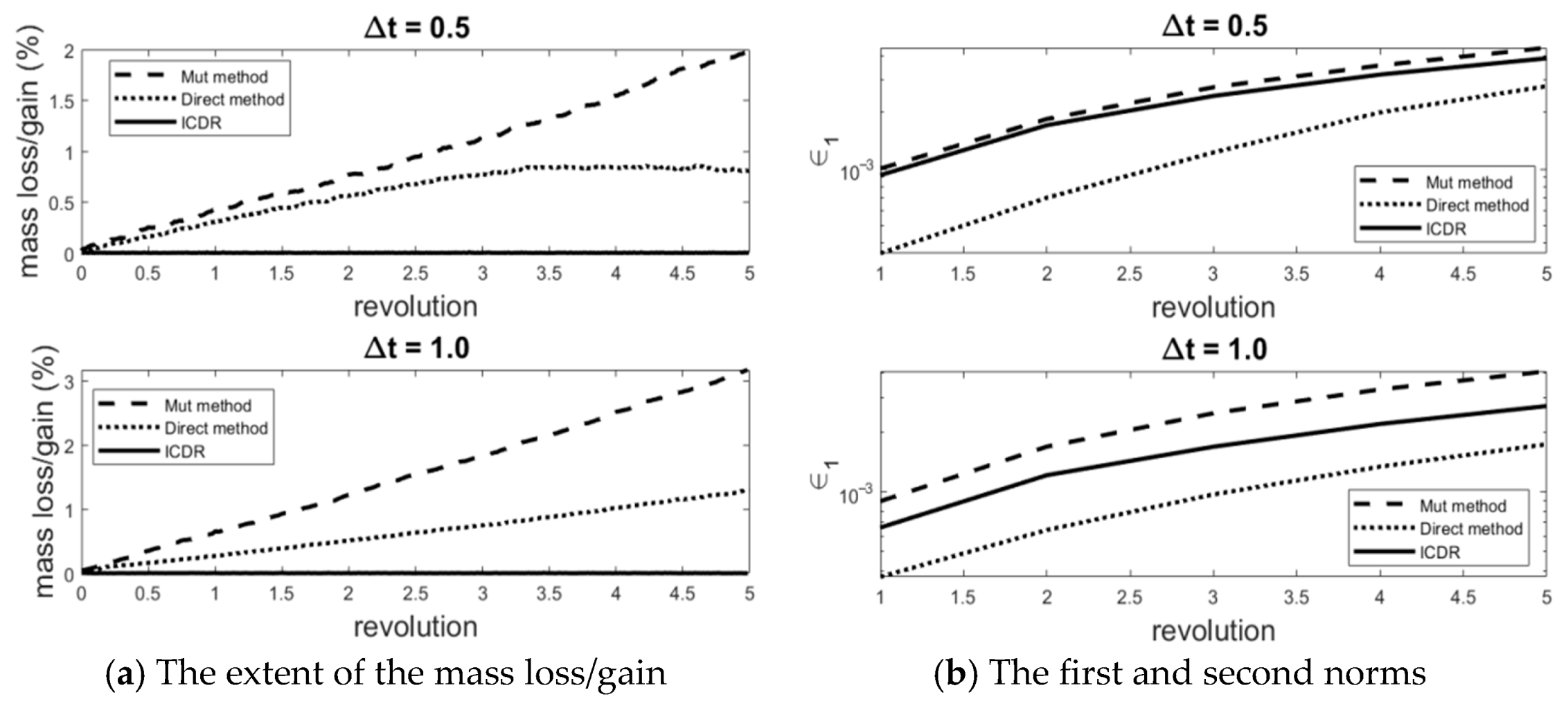
Besides the visual assessment of the different techniques in Figure 7a,b, the extent of mass loss/gain, and the norm values, are presented in Figure 8a,b to provide a quantitative evaluation. Figure 8a shows that the Mut method has more mass loss than the direct approach. Moreover, the ICDR method has nearly no mass loss/gain due to the global mass correction stated in Equation (18). Figure 8b reveals that the norm values are roughly similar for the ICDR and the Mut methods, and the direct approach has the lowest values. However, this does not mean that the direct method provides better results when considering the reconstructed shapes in Figure 7a,b. Notably, the value of the norm for the Mut approach using rectangular mesh is ${ϵ}_1=1.00\times {10}^{-3}$, which is very close to the calculated value using triangular meshes [24] (${ϵ}_1=1.2\times {10}^{-3}$).

4.2. The Notched Cylinder Problem

The displacement of a free surface, such as a notched cylinder’s revolution, comprises interface advection Equation (2) and interface re-initialization. Decreasing the time-step size ($\Delta t$) improves the interface advection’s accuracy; also, it increases the demand for the re-initialization step. The mass loss/gain during re-initialization and its correction can introduce some new sources of error. Therefore, small time-step sizes can decrease the accuracy due to the extra re-initialization steps.

To describe this problem in more detail, we examine different time steps in the allowable range ($\Delta t\le 2\Delta t^{*}$), based on Equation (8) for the notched cylinder problem. Moreover, we consider various structured mesh sizes $N_1\times N_2$, as depicted in Figure 1, to investigate the mesh dependency of the regenerated interface. The results are summarized in

Table 1. The values of the first norm (${ϵ}_1$) for different time steps and mesh spacings.

		${\mathit{N}}_1\times {\mathit{N}}_2$
		$50\times 50$	$100\times 100$	$200\times 200$	$300\times 300$	$400\times 400$	$500\times 500$
$\mathbf{\Delta }\mathit{t}$	$0.25\Delta t^{*}$	$1.80\times {10}^{-2}$	$4.17\times {10}^{-3}$	$9.14\times {10}^{-4}$	$7.52\times {10}^{-4}$	$7.59\times {10}^{-4}$	$7.60\times {10}^{-4}$
	$0.50\Delta t^{*}$	$1.13\times {10}^{-2}$	$4.10\times {10}^{-3}$	$7.51\times {10}^{-4}$	$5.61\times {10}^{-4}$	$4.64\times {10}^{-4}$	$4.19\times {10}^{-4}$
	$0.75\Delta t^{*}$	$7.90\times {10}^{-3}$	$2.58\times {10}^{-3}$	$6.36\times {10}^{-4}$	$5.11\times {10}^{-4}$	$4.58\times {10}^{-4}$	$4.05\times {10}^{-4}$
	$0.90\Delta t^{*}$	$8.00\times {10}^{-3}$	$2.48\times {10}^{-3}$	$6.22\times {10}^{-4}$	$4.75\times {10}^{-4}$	$4.17\times {10}^{-4}$	$3.62\times {10}^{-4}$
	$1.00\Delta t^{*}$	$7.90\times {10}^{-3}$	$2.43\times {10}^{-3}$	$6.20\times {10}^{-4}$	$4.57\times {10}^{-4}$	$3.75\times {10}^{-4}$	$3.32\times {10}^{-4}$
	$1.10\Delta t^{*}$	$8.71\times {10}^{-3}$	$2.50\times {10}^{-3}$	$6.65\times {10}^{-4}$	$5.37\times {10}^{-4}$	$4.71\times {10}^{-4}$	$4.34\times {10}^{-4}$
	$1.25\Delta t^{*}$	$1.03\times {10}^{-2}$	$2.85\times {10}^{-3}$	$7.58\times {10}^{-4}$	$5.66\times {10}^{-4}$	$6.36\times {10}^{-4}$	$4.77\times {10}^{-4}$
	$1.50\Delta t^{*}$	$1.52\times {10}^{-2}$	$3.94\times {10}^{-3}$	$9.41\times {10}^{-4}$	$6.71\times {10}^{-4}$	$7.04\times {10}^{-4}$	$5.49\times {10}^{-4}$
	$1.75\Delta t^{*}$	$204\times {10}^{-2}$	$5.08\times {10}^{-3}$	$1.22\times {10}^{-3}$	$8.66\times {10}^{-4}$	$7.51\times {10}^{-4}$	$7.14\times {10}^{-4}$
	$2.00\Delta t^{*}$	$2.56\times {10}^{-2}$	$6.69\times {10}^{-3}$	$1.66\times {10}^{-3}$	$1.22\times {10}^{-3}$	$1.07\times {10}^{-3}$	$1.03\times {10}^{-3}$

.

Table 1 quantitatively show that the increase or decrease of the time increment can destroy the results of an interface advection problem. However, there exists an optimum choice for the time increment ($\Delta t=1.00\Delta t^{*}$), which is highlighted by gray color in the tables. Notably, the solution is less sensitive to the time-step size when a finer mesh is employed. For example, for the cases with $N_1\times N_2=$ $300\times 300$, $400\times 400$, and $500\times 500$, time-step sizes in the range of $0.5\Delta t^{*}$ to $1.75\Delta t^{*}$ provide acceptable results.

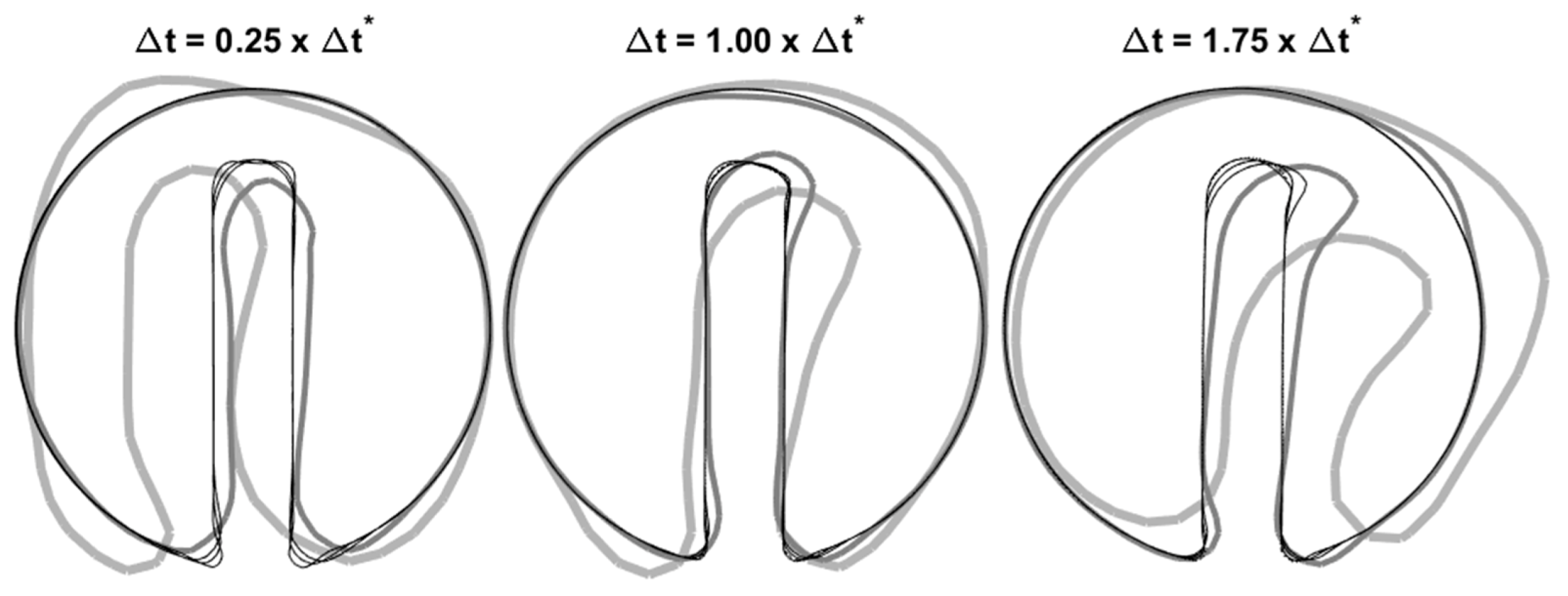
In Figure 9, we visually investigate the effect of the time-step size and mesh spacing by comparing the notched cylinder after one revolution. The thick lines with light grey and dark grey colors are for the cases with $N_1\times N_2=50\times 50$ and $100\times 100$, respectively. The regenerated interfaces in this figure reveal that the reconstructed surfaces are nearly similar when $N_1\times N_2\ge 200\times 200$. That is why it is difficult to distinguish between dashed, dash-dotted, dotted, and solid lines, which are for $200\times 200$, $300\times 300$, $400\times 400$, and $500\times 500$ meshing systems, respectively. The mesh independence of the results is more considerable for the case with $\Delta t=1.00\Delta t^{*}$. Notably, $\Delta t=1.00\Delta t^{*}$ is also the best choice for time-step size according to Table 1.

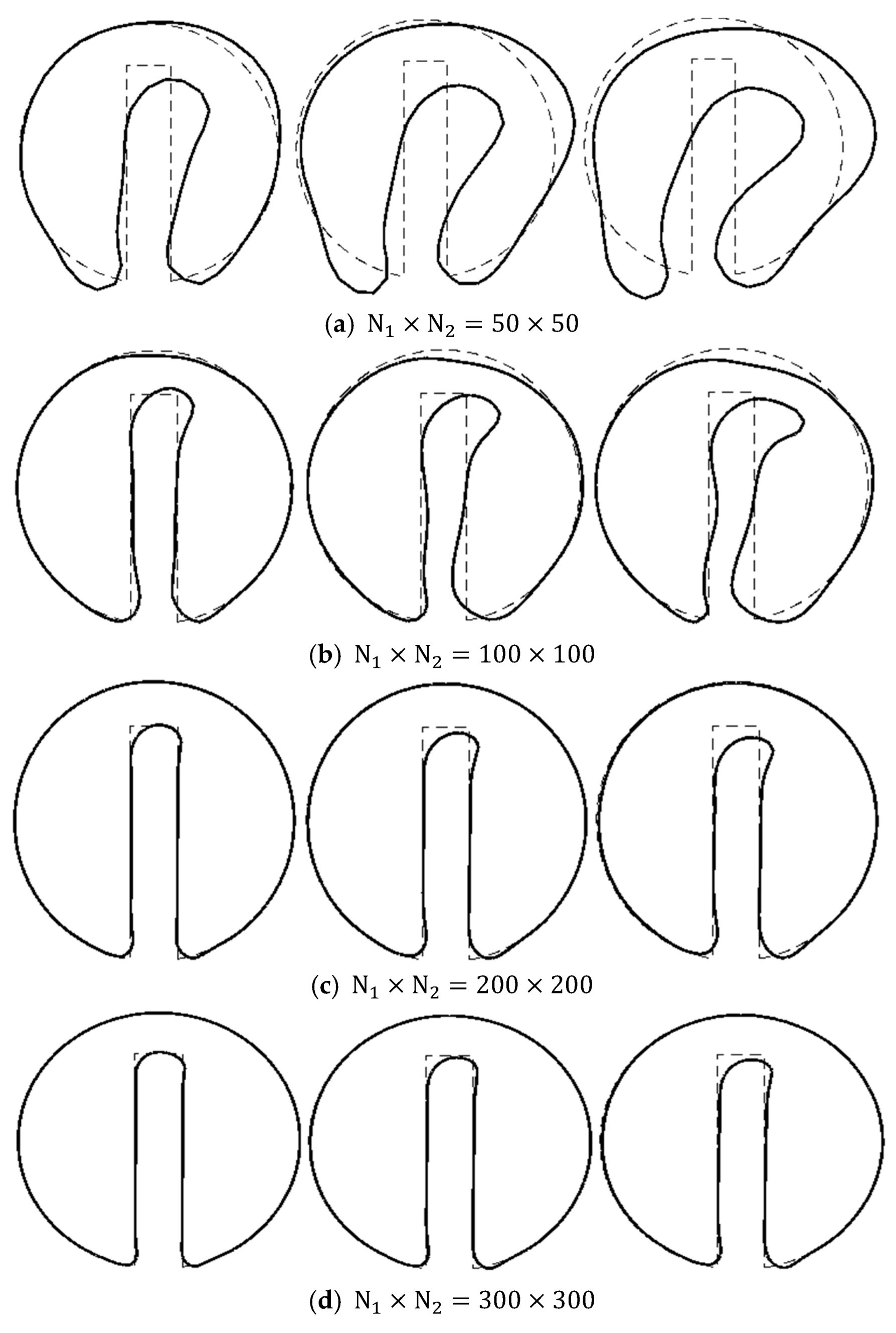
Now we take the best choice for the time step ($\Delta t=1.00\Delta t^{*}$), and visually investigate the mesh dependency of the regenerated notched cylinder after the first, third, and fifth revolution, in Figure 10a–f. The mesh dependency analysis in these figures shows that the interface prediction is improved by mesh refinement. Moreover, comparing the regenerated notched cylinders after the first, third and fifth revolutions shows an increasing deviation from the original shape over time (revolution), which is less significant for finner meshes.

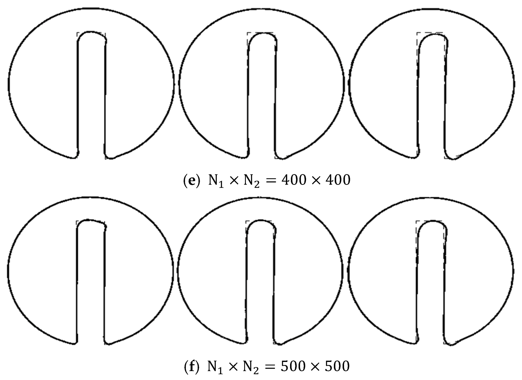
To quantify the observations of Figure 10, we show the defined norm value (${ϵ}_1$) during the revolutions for different mesh sizes in Figure 11a. These figures reveal that the mesh spacings of $50\times 50$ and $100\times 100$ do not provide a good prediction for the interface displacement. Moreover, for the range of $200<N_1$ the regenerated notched cylinders are nearly independent of the mesh size.

Although the main focus of this research is the geometrical re-initialization, we have provided some data based on the PDE re-initialization in Figure 11a. By comparing the norm values after the first revolution and PDE-based results, we can infer that the geometrical re-initialization does not always provide better results. However, the ICDR method leads to an acceptable solution (as discussed in the following sections) with less mathematical effort.

Figure 11b also shows the convergency order values for different mesh sizes and revolutions.

4.3. Swirling Flow Vortex

The swirling flow vortex is another benchmark problem used to evaluate the advection method and re-initialization scheme. This problem comprises a circle in a square flow domain, as introduced in Section 3.1. Similar to the notched cylinder problem, the flow field is independent of the interface shape. Equation (20a,b) define the velocity vectors’ components as a function of time and spatial coordinates. In this flow field, the circle stretches like a snake up to $t=T/2$, and after that time, it returns to its original position. In this research, we assume $T=8$.

$$u_1=-si{n}^2\left(\pi \left(x_1+0.5\right)\right)sin\left(2\pi \left(x_2+0.5\right)\right)cos\left(\pi t/T\right)$$

(20a)

$$u_2=-si{n}^2\left(\pi \left(x_2+0.5\right)\right)sin\left(2\pi \left(x_1+0.5\right)\right)cos\left(\pi t/T\right)$$

(20b)

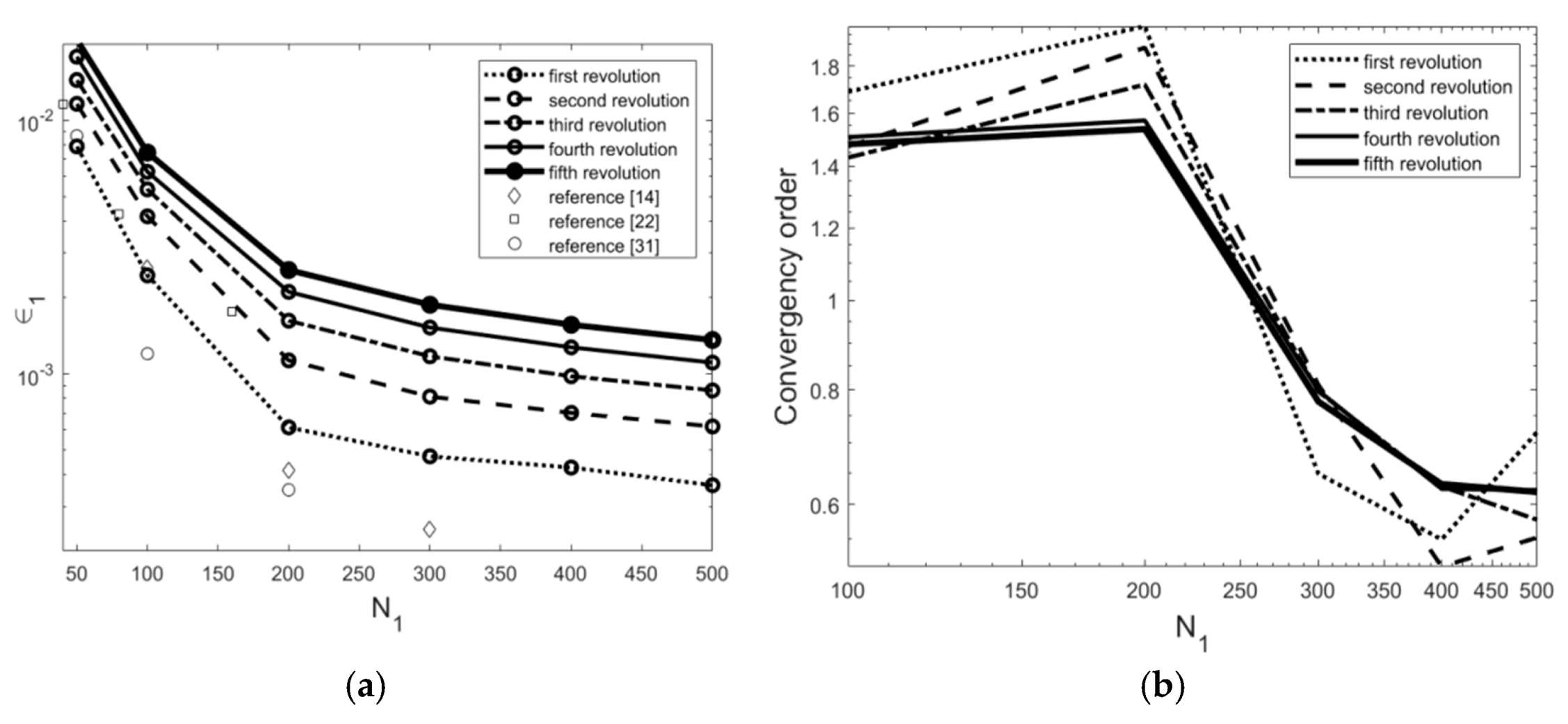
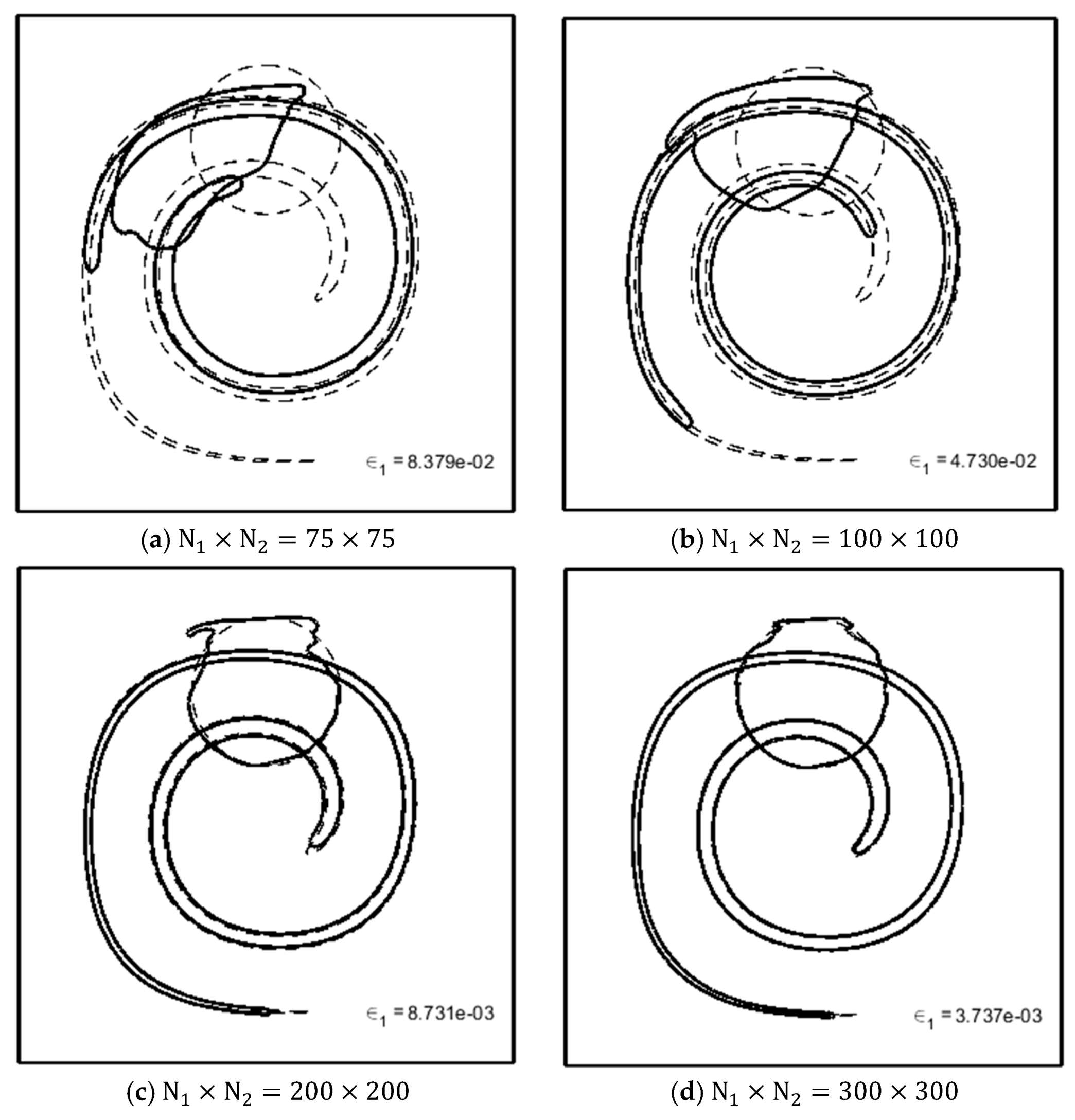
Figure 12a–f provide a graphical evaluation for the interface calculation results at $t=4$ and $t=T$ for structured meshes with different spacing. The dashed line shows the interface’s exact shape at the end of the stretching ($t=4$) and coming back ($t=8$) stages. These figures also contain the values of the defined norm for a quantitative comparison. The mesh dependency analysis in these figures shows that by decreasing the mesh sizes, better results for the interface prediction are achieved. However, we must consider the capacity of our computing system and calculation time before choosing a suitable grid spacing.

4.4. Unstructured Meshes

Notwithstanding that the description of the ICDR method in the Section 3 does not rely on a structured mesh, we provide some examples to evaluate the capability of the introduced method in unstructured meshes. In this section, we take the assumption of $\Delta t=\Delta t^{*}$. Note that the values of $N_1$ and $N_2$ are the integer part of the second root of the total element numbers.

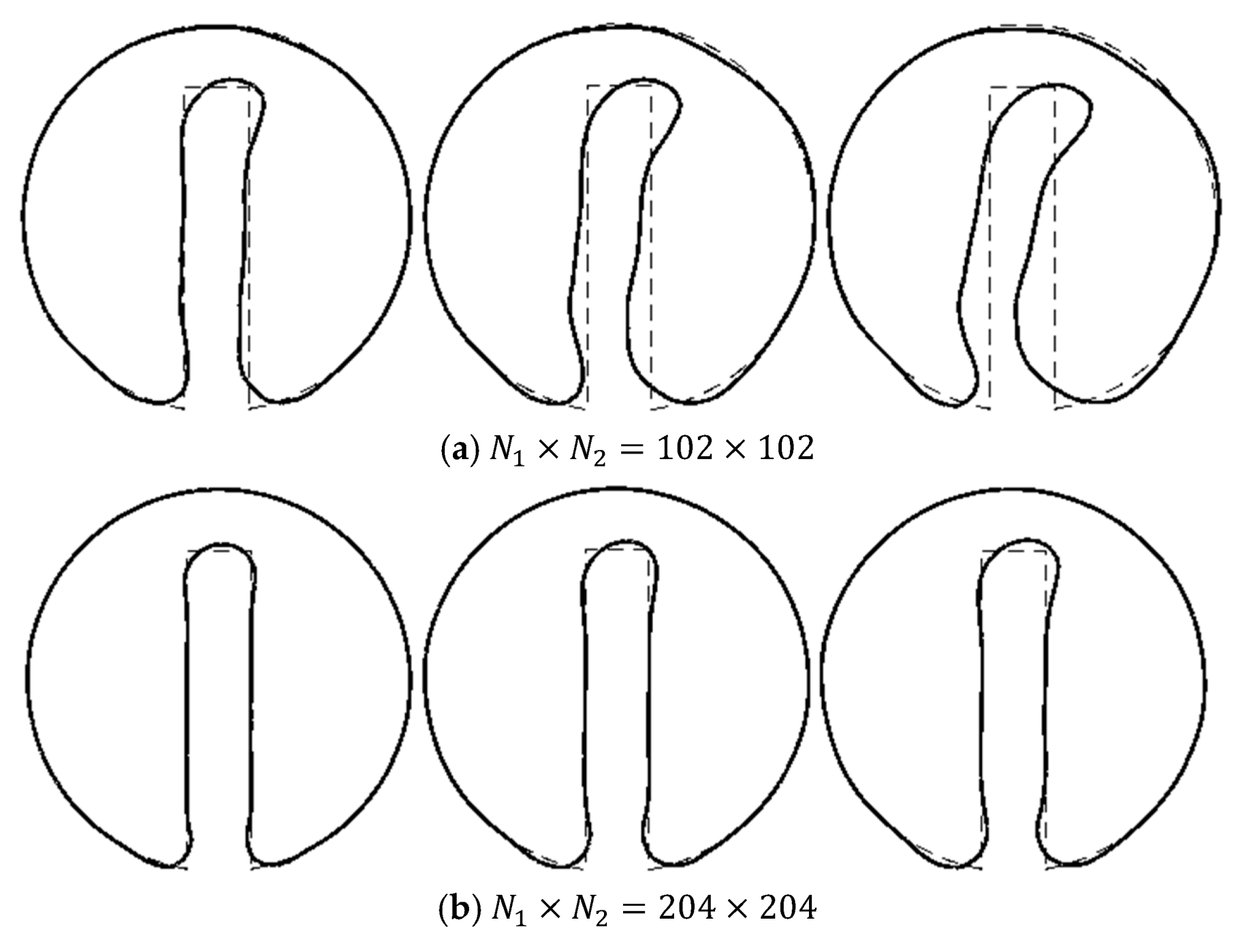
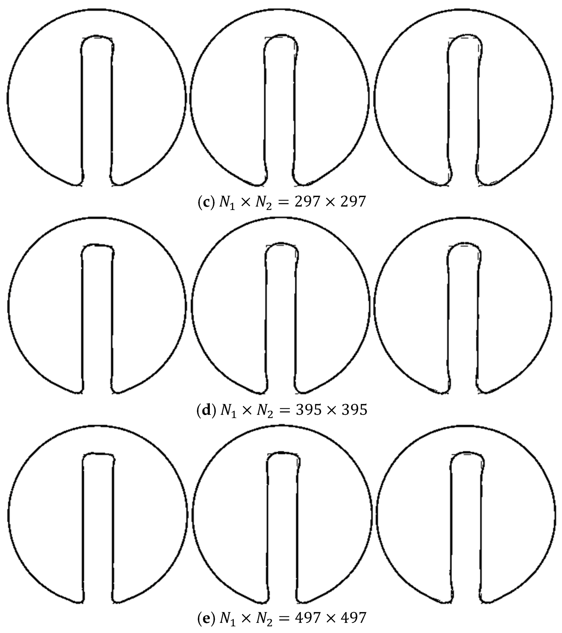
We start with the notched cylinder problem. To make the results visually comparable with corresponding regenerated interfaces in Figure 10, we have performed a mesh dependency analysis, as shown in Figure 13a–e. Similar to Figure 10, these figures show the regenerated notched cylinder after the first, third, and fifth revolutions.

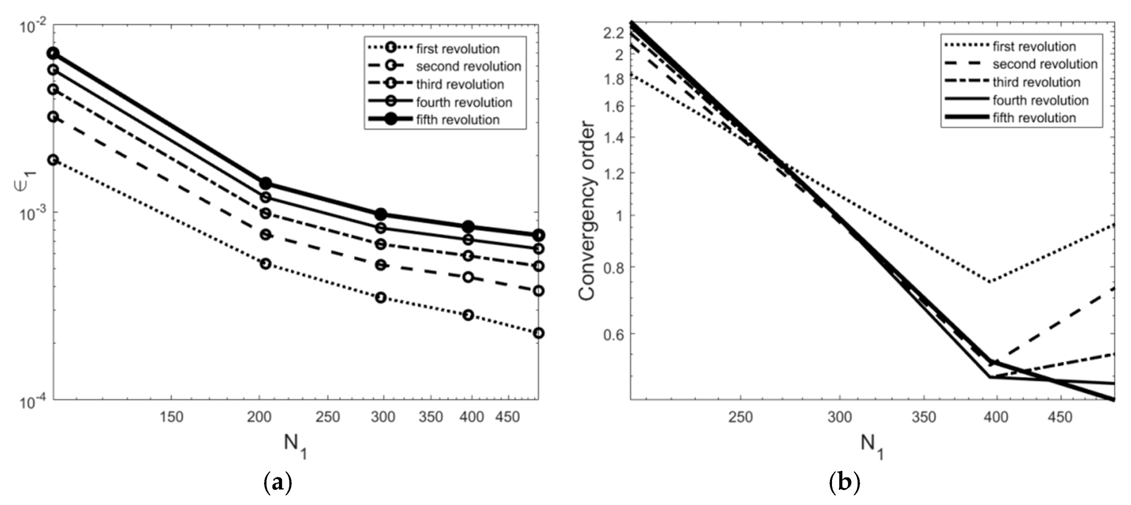
As it was reported for the structured meshes, we observe in Figure 13a–e that the reproduced interfaces comply better with the original shape by increasing the mesh numbers. To quantify the results of these figures, the values of the defined norm during the first to fifth revolutions are reported in Figure 14a,b also shows the order of the convergency for the ${ϵ}_1$ norm.

Figure 14a shows that for the range of $204<N_1$ the regenerated interfaces are nearly independent of the mesh size, similar to the cases with structure mesh in Figure 11. By comparing the data of Figure 11a and Figure 14a, we can surprisingly find that the values of the ${ϵ}_1$ norm of the unstructured meshes is less than the equivalent norms for the structured meshes.

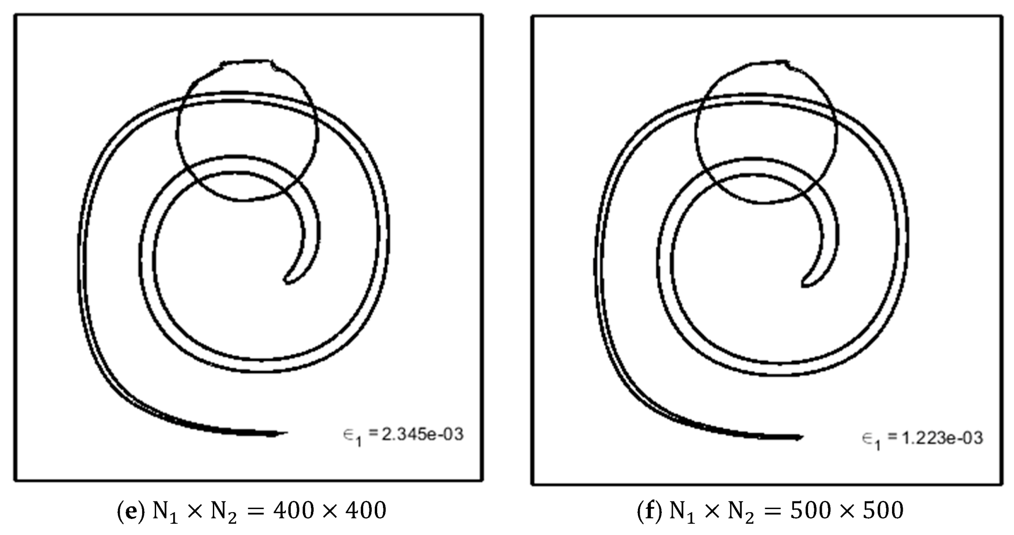
Figure 15a–e illustrate the results of our mesh dependency analysis for the swirling flow vortex using unstructured meshing systems. As expected, better results go for the cases with finer mesh. Paralleling the norm values in Figure 12 and Figure 15 reveals that for the swirling flow vortex problem, a structured mesh can provide better results.

4.5. The Extension to Three-Dimensional (3D) Problems

Aside from the benchmark problems, the main target of a re-initialization method is to predict the interface position in a physical phenomenon accurately. Various applications involve two-phase flow problems. However, we focus on the deformation of a drop (the second phase) in a simple shear flow. We have two reasons for this choice. The first reason is that in the drop deformation problem, despite the benchmark problems, the interface’s curvature influences the flow field via surface tension forces. Expectedly, an inaccurate interface displacement during re-initialization and mass correction can destroy the flow field calculations and the predicted drop shape. Therefore, a drop deformation problem is a good checkpoint for our re-initialization method. Secondly, there exist equivalent numerical and experimental data in the literature to compare our results with them and validate the ICDR method in 3D.

Figure 16 shows a typical two-phase simple shear flow field. In this picture, a drop with the radius of $R_{drop}$ is assumed in the middle of a channel with the dimensions of $\mathrm{W}\times \mathrm{H}\times \mathrm{L}$. The upper and lower plates are assumed to move in channel longitudinal direction with the velocities of $+U/2$ and $-U/2$; respectively. The extent of the drop deformation or breakup is a function of the viscosity ratio ($\lambda$) and Capillary number ($Ca$), which are defined in Equation (21a,b), where the parameters ${\mu }_1$ and ${\mu }_2$ show the viscosity of the matrix (the primary phase)and drop (the second phase), respectively. Moreover, the parameter $\mathsf{\gamma }$ stands for the surface tension coefficient.

$$\lambda =\frac{{\mu }_2}{{\mu }_1}$$

(21a)

$$Ca=\frac{{\mu }_1\left(U/H\right)R_{drop}}{\gamma }$$

(21b)

By taking the assumptions of the creeping flow and incompressible fluids, the governing equations, including the equation of motion and mass conservation criterion, would be as follows:

$$\frac{\partial {\sigma }_{ij}}{\partial x_j}=F_{{\sigma }_i}$$

(22a)

$$\frac{\partial u_i}{\partial x_i}=0$$

(22b)

The Equation (22a,b) are based on Einstein summation notations over a common index. The components of the total stress tensor ($\stackrel{=}{\mathbf{\sigma }}$) are denoted by ${\sigma }_{ij}$, which are described in Equation (23a–c).

$${\sigma }_{ij}={\tau }_{ij}+P{I}_{ij}$$

(23a)

$${\tau }_{ij}=-\mu D_{ij}$$

(23b)

$$D_{ij}=\frac{\partial u_i}{\partial x_j}+\frac{\partial u_j}{\partial x_i}$$

(23c)

where ${\tau }_{ij}$ and $D_{ij}$ are components of the viscous stress ($\stackrel{=}{\mathit{\tau }}$) and deformation rate ($\stackrel{=}{\mathit{D}}$) tensors; respectively. $P$ and $\mu$ are hydrostatic pressure and Newtonian viscosity, correspondingly. $I_{ij}$ is the unit tensor ($I$) component (Kronecker delta), such that $I_{ij}$ is 1 if $i=j$ and is 0 if $i\ne j$.

$F_{{\sigma }_i}$ in Equation (21a) is the component of the surface tension force per unit volume (${\overrightarrow{\mathit{F}}}_{\mathit{\sigma }}$) and is easily calculated using Equation (23) [32].

$${\overrightarrow{\mathit{F}}}_{\mathit{\sigma }}=\gamma \kappa \overrightarrow{\mathit{n}}$$

(24)

The solution strategy is to employ the Galerkin finite element method (FEM) for Equation (22a,b). Moreover, we consider a periodic boundary condition on the front/back and the left/right sides. The surface tension force (${\overrightarrow{\mathit{F}}}_{\mathit{\sigma }}$) is considered as a source term, which is non-zero in the active elements. Mostafaiyan et al. have described the solution method’s detail (for the two-dimensional case) in [7].

Our setup in this section is to employ a structured mesh in the flow domain with hexagonal elements. We assume 40 grids in the depth of the channel (element size is $\mathrm{H}/40$), for which we have obtained mesh-independent results in our two-dimensional analysis [7]. We assume the time increment to be slightly smaller than the characteristic time (e.g., $\Delta \mathrm{t}=0.9\Delta t^{*}$).

In this section, we examine the proposed method by juxtaposing our results with some numerical and experimental data in the literature. For this purpose, the extent of the drop deformation and its breakup are presented for unit and non-unit viscosity ratios.

4.5.1. Comparison of the Geometrical Re-Initialization Methods in 3D

We consider a case with $Ca=0.4$ and $2R_{drop}=0.5H$. Figure 17a shows the results of our calculations, which are re-initialized using the ICDR method. In this figure, a binary breakup is observed, which complies with the reported data in [33] (Figure 13). Notably, for this problem the Capillary number of $0.4$ is a critical value, below which no break up will happen [33].

Simulation of the problem using the Mut method does not lead to a breakup, as shown in Figure 17b. The simulation time equals in Figure 17a,b. However, in the recent case, the drop reaches its equilibrium before any breakup. We attribute the difference between the two figures to the second phase’s mass loss during deformation. The drop losses part of its mass and converts to a smaller one (i.e., a drop with a smaller $R_{drop}$) in the simulation course. Thus, according to Equation (21b), the Capillary number drops below the critical value and will not break up, as a result.

We have also employed the direct re-initialization algorithm to estimate the extent of the drop deformation. In this case, the interface is destroyed during the deformation, as shown in Figure 17c, and we cannot continue simulation up to the breakup time in Figure 17a, due to the numerical errors. The unsuccessful simulation’s main reason is the inaccurate prediction of the surface tension forces due to the volume fraction’s unsmooth values in the interface’s vicinity. It is worth reminding that the active elements’ nodal values are not re-initialized in the direct algorithm.

4.5.2. Case Study for Drop Deformation with a Unit Viscosity Ratio

Figure 17a shows that our analysis complies with the numerical results in the literature [33]. In this section, we use our two-phase flow strategy to simulate an experimental task of Sibillo et al. [34] with $2R_{drop}=0.7H$ and $Ca=0.46$. Their result (a quinary breakup) are reproduced by our simulation and compared in Figure 18a,b.

4.5.3. Case Study for Drop Deformation with Non-Unit Viscosity Ratios

Since the flow field contains two different fluids with the viscosity values of ${\mu }_1$ and ${\mu }_2$ (${\mu }_1\ne {\mu }_2$), an appropriate viscosity estimation ($\mu$) in Equation (23b) is required. We have estimated the viscosity using the area portion of an element occupied by the primary and second phases, as shown in Equation (25a,b).

$$\mu =f_e{\mu }_1+\left(1-f_e\right){\mu }_2$$

(25a)

$$f_e=\frac{{\int }_{{\Omega }_e}^{}\lfloor \langle \varphi \rangle \left\{f_i\right\}+\frac{1}{2}\rfloor d{x}_{1}d{x}_2}{{\int }_{{\Omega }_e}^{}d{x}_{1}d{x}_2}$$

(25b)

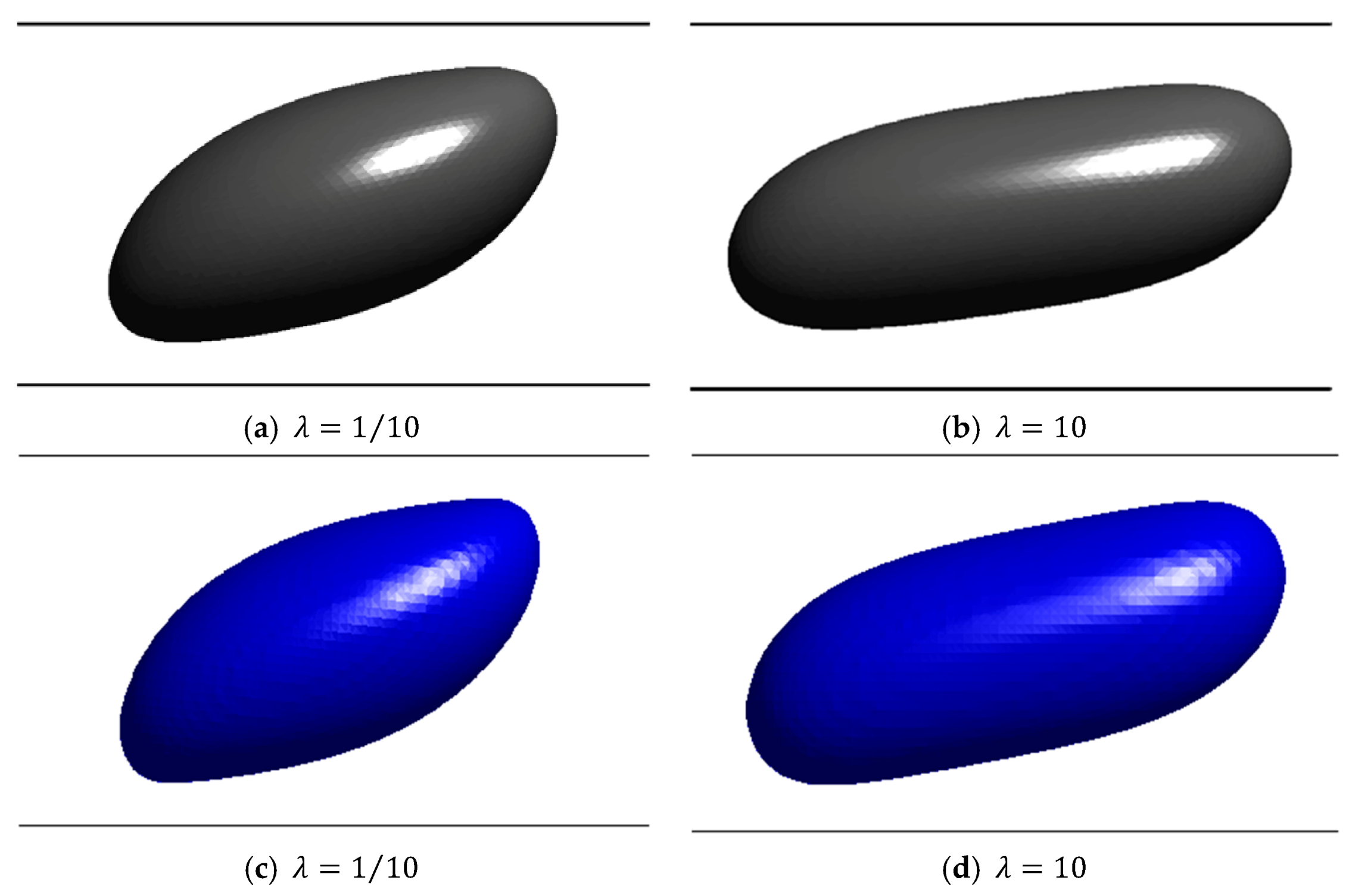
To evaluate our re-initialization method for problems with non-unit viscosity ratio, we evaluate the steady shape a drop with $2R_{drop}=0.9H$ and $Ca=0.3$ for different viscosity ratios (i.e., $\lambda =10$ and $\lambda =1/10$) and compare it with similar data in the literature. Figure 19a,b show the shape of the drops at equilibrium, generated using the Boundary-integral method [35]. Figure 19c,d present the corresponding results while using our finite element strategy.

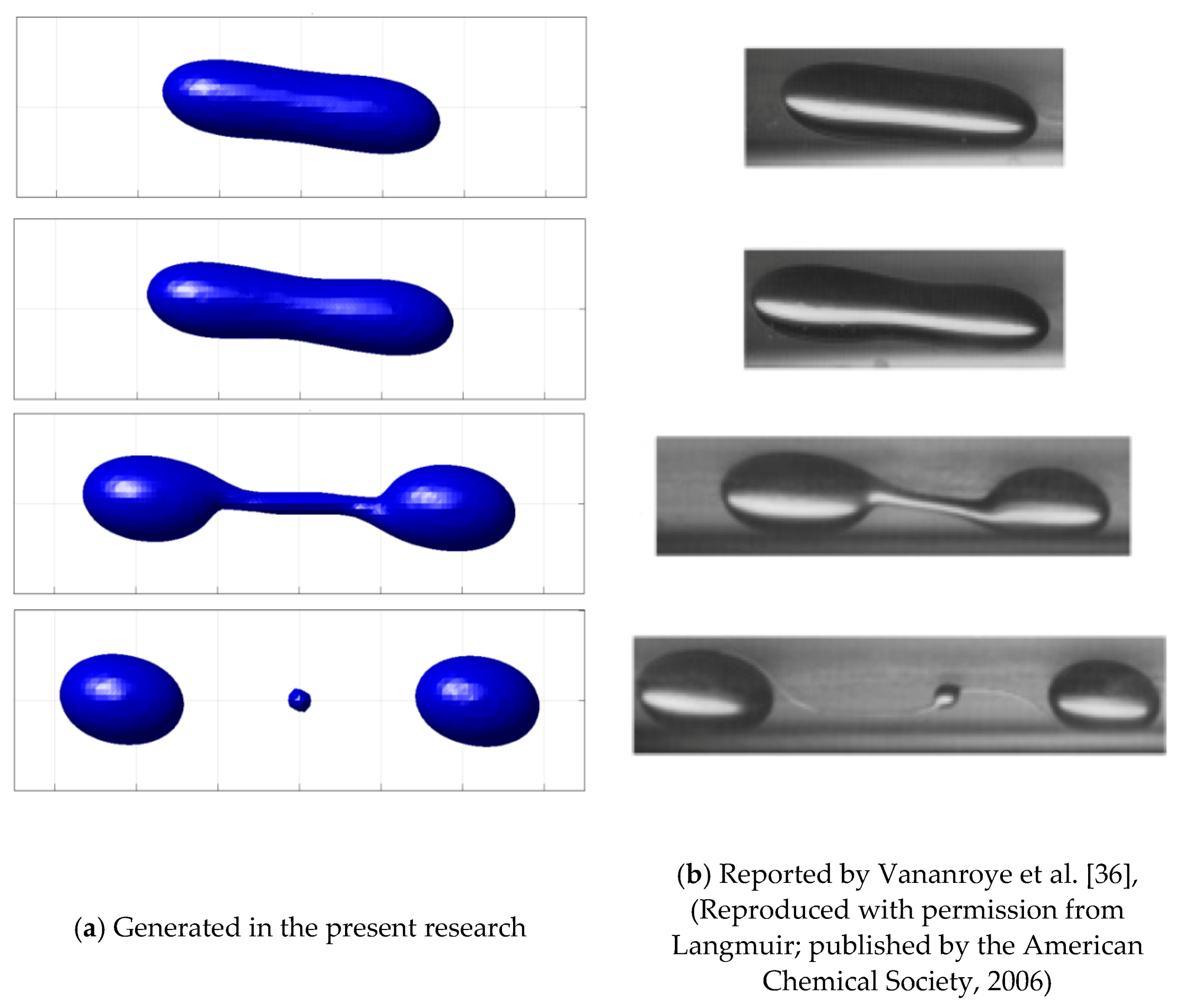
For drop deformation with a non-unit viscosity ratio, the breakup is possible. Vananroye et al. [36] have experimentally reported such a breakup for a drop with $2R_{drop}=0.75H$, $Ca=0.6$, and $\lambda =11.7$, as shown in Figure 20b. Figure 20a depicts the reproduced results using our FEM formulation and the ICDR technique.

The similarity between our calculations and different experimental and numerical data in the literature ($\lambda =1$ or $\lambda \ne 1$) reflects the ICDR technique’s capability in conjunction with our FEM in analyzing two-phase flow problems.

It is worth mentioning that we have performed several successful comparisons for the drop deformation problems (with the unit and non-unit viscosity ratios). However, they are not reported here for conciseness.

5. Conclusions

We have introduced an improved mass-conservative direct re-initialization method (ICDR) based on two existing geometrical re-initialization methods (the Mut and the direct method) and a global mass correction concept. This method has excellent mass-conservative properties and provides a smooth set of nodal volume fractions in the interface’s vicinity. We have shown that the ICDR method is applicable for 2D and 3D flow problems.

To assess the validity of the ICDR method in 2D, we have employed two benchmark problems. Then the dependency of the results on the element and time-step size has been extensively examined. A visual assessment using graphical demonstrations of the regenerated interfaces, as well as a quantitative evaluation via the definition of a norm value, have been provided.

Aside from the benchmark problems, we have decided to use an actual physical phenomenon to examine the ICDR method’s applicability in 3D. For this purpose, a drop deformation in a simple shear flow field has been selected. Comparing our results with various numerical and experimental data in the literature has shown that, using the introduced strategy, one can predict the droplet equilibrium or break up for unit and non-unit viscosity ratios.

The 3D flow fields in this research are limited to creeping flow. However, the ICDR algorithm’s evaluation by considering the inertial terms (e.g., bubble rising and dam-break problems) can be a subject of further studies.

References

- Osher, S.; Sethian, J.A. Fronts propagating with curvature-dependent speed: Algorithms based on Hamilton-Jacobi formulations. J. Comput. Phys. 1988, 79, 12–49. [Google Scholar] [CrossRef] [Green Version]
- Hirt, C.W.; Nichols, B.D. Volume of fluid (VOF) method for the dynamics of free boundaries. J. Comput. Phys. 1981, 39, 201–225. [Google Scholar] [CrossRef]
- Pilliod, J.E., Jr.; Puckett, E.G. Second-order accurate volume-of-fluid algorithms for tracking material interfaces. J. Comput. Phys. 2004, 199, 465–502. [Google Scholar] [CrossRef] [Green Version]
- Pilliod, J.; Puckett, E. An unsplit, second-order accurate Godunov method for tracking deflagrations and detonations. In Proceedings of the 21st International Symposium on Shock Waves, Center for Hypersonics, Great Keppel Island, Australia, 20–25 July 1997; pp. 1053–1058. [Google Scholar]
- Puckett, E. On the second-order accuracy of volume-of-fluid interface reconstruction algorithms: Convergence in the max norm. Commun. Appl. Math. Comput. Sci. 2010, 5, 99–148. [Google Scholar] [CrossRef]
- Puckett, E.A. Volume-of-fluid interface reconstruction algorithm that is second-order accurate in the max norm. Commun. Appl. Math. Comput. Sci. 2010, 5, 199–220. [Google Scholar] [CrossRef] [Green Version]
- Mostafaiyan, M.; Wießner, S.; Heinrich, G.; Hosseini, M.S.; Domurath, J.; Khonakdar, H.A. Application of local least squares finite element method (LLSFEM) in the interface capturing of two-phase flow systems. Comput. Fluids 2018, 174, 110–121. [Google Scholar] [CrossRef]
- Smereka, P.; Sussman, M.; Osher, S. A levelset approach for computing solutions to incompressible two-phase flow. J. Comput. Phys. 1994, 114, 1006. [Google Scholar]
- Chang, Y.-C.; Hou, T.; Merriman, B.; Osher, S. A level set formulation of Eulerian interface capturing methods for incompressible fluid flows. J. Comput. Phys. 1996, 124, 449–464. [Google Scholar] [CrossRef] [Green Version]
- Sussman, M.; Fatemi, E.; Smereka, P.; Osher, S. An improved level set method for incompressible two-phase flows. Comput. Fluids 1998, 27, 663–680. [Google Scholar] [CrossRef]
- Sussman, M.; Fatemi, E. An efficient, interface-preserving level set redistancing algorithm and its application to interfacial incompressible fluid flow. SIAM J. Sci. Comput. 1999, 20, 1165–1191. [Google Scholar] [CrossRef] [Green Version]
- Yap, Y.; Chai, J.; Wong, T.; Toh, K.; Zhang, H. A global mass correction scheme for the level-set method. Numeric. Heat Transf. Part B Fundam. 2006, 50, 455–472. [Google Scholar] [CrossRef]
- Ville, L.; Silva, L.; Coupez, T. Convected level set method for the numerical simulation of fluid buckling. Int. J. Numeric. Methods Fluids 2011, 66, 324–344. [Google Scholar] [CrossRef]
- Olsson, E.; Kreiss, G. A conservative level set method for two phase flow. J. Comput. Phys. 2005, 210, 225–246. [Google Scholar] [CrossRef]
- Olsson, E.; Kreiss, G.; Zahedi, S.A. conservative level set method for two phase flow II. J Comput. Phys 2007, 225, 785–807. [Google Scholar] [CrossRef]
- Harten, A. The artificial compression method for computation of shocks and contact discontinuities. I. Single conservation laws. Commun. Pure App. Math. 1977, 30, 611–638. [Google Scholar] [CrossRef]
- Zhao, L.; Mao, J.; Bai, X.; Liu, X.; Li, T.; Williams, J. Finite element implementation of an improved conservative level set method for two-phase flow. Comput. Fluids 2014, 100, 138–154. [Google Scholar] [CrossRef]
- Zhao, L.; Bai, X.; Li, T.; Williams, J. Improved conservative level set method. Int. J. Numeric. Methods Fluids 2014, 75, 575–590. [Google Scholar] [CrossRef]
- Guermond, J.-L.; de Luna, M.Q.; Thompson, T. An conservative anti-diffusion technique for the level set method. J. Computat. Appl. Math. 2017, 321, 448–468. [Google Scholar] [CrossRef] [Green Version]
- Chiodi, R.; Desjardins, O. A reformulation of the conservative level set reinitialization equation for accurate and robust simulation of complex multiphase flows. J. Comput. Phys. 2017, 343, 186–200. [Google Scholar] [CrossRef]
- Enright, D.; Fedkiw, R.; Ferziger, J.; Mitchell, I. A hybrid particle level set method for improved interface capturing. J. Comput. Phys. 2002, 183, 83–116. [Google Scholar] [CrossRef] [Green Version]
- Wang, Z.; Yang, J.; Stern, F. An improved particle correction procedure for the particle level set method. J. Comput. Phys. 2009, 228, 5819–5837. [Google Scholar] [CrossRef]
- Sussman, M.; Puckett, E.G. A coupled level set and volume-of-fluid method for computing 3D and axisymmetric incompressible two-phase flows. J. Comput. Phys. 2000, 162, 301–337. [Google Scholar] [CrossRef] [Green Version]
- Mut, F.; Buscaglia, G.C.; Dari, E.A. New mass-conserving algorithm for level set redistancing on unstructured meshes. J. Appl. Mechan. 2006, 73, 1659–1678. [Google Scholar] [CrossRef] [Green Version]
- Ausas, R.F.; Dari, E.A.; Buscaglia, G.C. A geometric mass-preserving redistancing scheme for the level set function. Int. J. Numeric. Methods Fluids 2011, 65, 989–1010. [Google Scholar] [CrossRef]
- Cho, M.H.; Choi, H.G.; Yoo, J.Y. A direct reinitialization approach of level-set/splitting finite element method for simulating incompressible two-phase flows. Int. J. Numeric. Methods Fluids 2011, 67, 1637–1654. [Google Scholar] [CrossRef]
- Ngo, L.C.; Choi, H.G. Efficient direct re-initialization approach of a level set method for unstructured meshes. Comput. Fluids 2017, 154, 167–183. [Google Scholar] [CrossRef]
- Chopp, D.L. Computing minimal surfaces via level set curvature flow. J. Comput. Phys. 1993, 106, 77–91. [Google Scholar] [CrossRef] [Green Version]
- Jiang, B.-N. The Least-Squares Finite Element Method: Theory and Applications in Computational Fluid Dynamics and Electromagnetics; Springer: Berlin/Heidelberg, Germany, 1998. [Google Scholar]
- Zalesak, S.T. Fully multidimensional flux-corrected transport algorithms for fluids. J. Comput. Phys. 1979, 31, 335–362. [Google Scholar] [CrossRef]
- Walker, C.; Müller, B. A conservative level set method for sharp interface multiphase flow simulation. In Proceedings of the ECCOMAS CFD, Lisbon, Portugal, 14–17 June 2010. [Google Scholar]
- Tryggvason, G.; Bunner, B.; Esmaeeli, A.; Juric, D.; Al-Rawahi, N.; Tauber, W.; Han, J.; Nas, S.; Jan, Y.-J. A front-tracking method for the computations of multiphase flow. J. Comput. Phys. 2001, 169, 708–759. [Google Scholar] [CrossRef] [Green Version]
- Janssen, P.; Anderson, P. Boundary-integral method for drop deformation between parallel plates. Phys. Fluids 2007, 19, 043602. [Google Scholar] [CrossRef] [Green Version]
- Sibillo, V.; Pasquariello, G.; Simeone, M.; Cristini, V.; Guido, S. Drop deformation in microconfined shear flow. Phys. Rev. Lett. 2006, 97, 054502. [Google Scholar] [CrossRef]
- Janssen, P.; Anderson, P. A boundary-integral model for drop deformation between two parallel plates with non-unit viscosity ratio drops. J. Comput. Phys. 2008, 227, 8807–8819. [Google Scholar] [CrossRef]
- Vananroye, A.; Van Puyvelde, P.; Moldenaers, P. Effect of confinement on droplet breakup in sheared emulsions. Langmuir 2006, 22, 3972–3974. [Google Scholar] [CrossRef]
Figure 1.
The interface and the elements in its vicinity.
Figure 2.
An arbitrary 3D element.
Figure 3.
Two revolutions of a circle using a structured mesh, where the nodes of active elements are included in the re-initialization step (a) An original circle before (dashed line) and after two revolutions (solid line). The normal vectors are shown after rotation, (b) The percentage of curvature deviation (solid line) and mass change (dashed line).
Figure 4.
Five revolutions of a circle using a structured mesh, using the direct method (a) An original circle before (dashed line) and after five revolutions (solid line). The normal vectors are shown after rotation, (b) The percentage of curvature deviation (solid line) and mass change (dashed line).
Figure 5.
Five revolutions of a circle using a structured mesh, using the Mut method (a) An original circle before (dashed line) and after five revolutions (solid line). The normal vectors are shown after rotation, (b) The percentage of curvature deviation (solid line) and mass change (dashed line).
Figure 6.
Five revolutions of a circle using a structured mesh, using the improved conservative direct re-initialization or ICDR (a) An original circle before (dashed line) and after five revolutions (solid line). The normal vectors are shown after rotation, (b) The percentage of curvature deviation (solid line) and mass change (dashed line).
Figure 7.
Revolution of the notched cylinder in a rectangular domain. In these figures, the dashed line shows the original shape. Also, the solid line and dotted line are the results for ∆t = 0.5 and ∆t = 1.0, respectively.
Figure 8.
Comparison of the mass loss/gain and the norm values for different methods.
Figure 9.
The reconstructed notched cylinder after one revolution for different time increments () and mesh spacing: (light-grey), (dark-grey), (dashed), (dash-dotted), (dotted), (solid line).
Figure 10.
The Notched cylinder after first (left picture), third (middle picture), and fifth (right picture) revolutions with different structured mesh spacing. The solid lines show the results after the evolutions and the dashed lines are the original notched cylinder.
Figure 11.
(a), The values of the norm during the revolutions for various structured mesh spacing, as well as the comparison with PDE-based re-initialization methods [14,22,31] (b), The values of the convergency order during the revolutions for various structured mesh spacing.
Figure 12.
The interface shape in swirling flow vortex at and for structured meshes with different spacing. The values of the norm is also presented.
Figure 13.
The Notched cylinder after first (left picture), third (middle picture) and fifth (right picture) revolutions with different unstructured mesh spacing. The solid lines show the results after the evolutions and the dashed lines are the original notched cylinder.
Figure 14.
(a), The values of the norm during the revolutions for various structured mesh spacing, (b), The values of the convergency order during the revolutions for various structured mesh spacing.
Figure 15.
The interface shape in swirling flow vortex at t = 4 and t = 8 for unstructured meshes with different spacing. The values of the norm is also presented.
Figure 16.
A schematic illustration of the two-phase simple shear flow.
Figure 17.
The shapes of the drops with the diameter of and Ca = 0.4, (a): ICDR, (b): Mut et al. [1], (c): Direct re-initialization [2,3].
Figure 18.
The evolution of the drop shape with the diameter of and the Capillary number of , (a): Generated in the present research, (b): Reported by Sibillo et al. [34], (Reproduced with permission from physical review letters; published by the American Physical Society, 2006).
Figure 19.
The steady shapes of the drops with the diameter of and for different values of the viscosity ratios (λ = 0.1 and 10), (a,b): Reported by Janssen and Anderson [35] (Reproduced with permission from Author; published by Elsevier, 2008), (c,d): Generated in the present research.
Figure 20.
The different states of the deformation before the breakup of a drop with , , and .