Aerodynamic Prediction of Time Duration to Becoming Infected with Coronavirus in a Public Place

Abstract

The COVID-19 pandemic has caused panic and chaos that modern society has never seen before. Despite their paramount importance, the transmission routes of coronavirus SARS-CoV-2 remain unclear and a point of contention between the various sectors. Recent studies strongly suggest that COVID-19 could be transmitted via air in inadequately ventilated environments. The present study investigates the possibility of the aerosol transmission of coronavirus SARS-CoV-2 and illustrates the associated environmental conditions. The main objective of the current work is to accurately predict the time duration of getting an infection while sharing an indoor space with a patient of COVID-19 or similar viruses. We conducted a 3D computational fluid dynamics (CFD)-based investigation of indoor airflow and the associated aerosol transport in a restaurant setting, where likely cases of airflow-induced infection of COVID-19 caused by asymptomatic individuals were reported in Guangzhou, China. The Eulerian–Eulerian flow model coupled with the k-Ɛ turbulence approach was employed to resolve complex indoor processes, including human respiration activities, such as breathing, speaking, and sneezing. The predicted results suggest that 10 minutes are enough to become infected with COVID-19 when sharing a Table with coronavirus patients. The results also showed that although changing the ventilation rate will improve the quality of air within closed spaces, it will not be enough to protect a person from COVID-19. This model may be suitable for future engineering analyses aimed at reshaping public spaces and indoor common areas to face the spread of aerosols and droplets that may contain pathogens.

1. Introduction

Coronavirus SARS-CoV-2 continues to spread throughout the world, keeping people and businesses shuttered. The virus is obviously something to be scared of. As of April 2022, there have been more than 497 million cases of coronavirus (COVID-19) and over 6.17 million deaths worldwide. The coronaviruses are a large family of viruses that cause illness in animals and humans. In humans, coronaviruses can cause respiratory infections such as the common cold as well as more series diseases, such as Middle East Respiratory Syndrome (MERS) and Severe Acute Respiratory Syndrome (SARS). COVID-19 is an infectious disease caused by a new form of coronavirus called SARS-CoV-2 [1,2]. It was first reported in December 2019 in Wuhan City in China [3,4]. SARS-CoV2 never travels alone but always in an aqueous environment [4,5,6]. Early studies assumed that the transmission of the virus between humans occurs only through direct contact with an infected individual [3,7]. However, recent evidence strongly suggests that COVID-19 could be transmitted via air in inadequately ventilated environments [8,9,10,11,12].

Breathing, speaking, coughing, sneezing, and laughing all cause thousands of droplets and aerosols to be released into the air [4]. Depending on the type of activity, the number, velocity, and size distributions of droplets vary. Droplets’ characteristics such as concentration and size, have significant implications on the transmission process of these droplets. Smaller droplets, which carry fewer particles, can remain suspended in the air for hours, while larger droplets, which carry more viruses, will settle quicker due to gravity. Therefore, this topic has attracted a lot of attention and has become the focus of many recent studies [13,14,15,16,17,18,19,20]. These studies were conducted on a group of healthy individuals [13,14,15,16,18,19] from a group of subjects who were infected with influenza [17]. The results of these studies showed that normal breathing can produce an order of 10³ or more droplets per liter, with an average size varying from 0.3 to 5 µm. The results of these studies also showed that speaking may release 10 times more droplets into the air, with average size varying from 5 to 75 µm [13,14]. However, it is worthy of mentioning that some of these studies found that most of the particles were less than 1 µm in diameter during expiratory activities [15,19].

The majority of early studies on this topic concluded that there is no evidence of SARS-CoV-2 airborne transmission [3,21,22,23]. In the middle of 2020, several studies discussed the possibility of airborne transmission of SARS-CoV-2 [4,8,9,10,11,12,24]. These studies provided insightful arguments about the possibility of virus transmission to healthy individuals through the inhalation of air mixed with droplets containing the virus. There is some evidence that the inertial forces due to airflow and drag on the droplet and gravitational sedimentation have a considerable impact on aerosol transport within a control volume. The forces acting on a droplet primarily depend on droplet size and its position in the flow field. Brownian force plays a significant role in the aerosol transportation of small droplets (<0.5 μm). However, this effect becomes less important with increased droplet size. The first attempt to simulate and investigate the indoor airflow and the associated aerosol transport was made by [25]. However, this model was not specifically designed to predict the number of droplets inhaled and evaluate the maximum time you can stay in such places. Wang et al. [26] conducted a numerical investigation to study the transmission process of the SARS-CoV-2 during two actual flights. They simulated the dispersion of respiratory droplets of different sizes generated by an infected person. The predicted results showed that wearing masks and reducing conversation between passengers could help to reduce the risk of becoming infected.

More recent attention has focused on the use of computational fluid dynamics (CFD) to investigate the aerosol transport of SARS-CoV-2 in indoor and outdoor environments [24,27,28,29,30,31]. Many countries worldwide have taken early measures to combat the spread of the virus by implementing social distancing measures. In addition to that, wearing a face mask became mandatory whenever you cannot apply the social distancing measures. Furthermore, it was mandatory to wear a face mask in indoor settings such as on public transport, in taxis, and in the classroom. Despite this, it is difficult to apply this rule while dining in a restaurant. Therefore, the main objective of the present study is to investigate aerosol transport of SARS-CoV-2 in a restaurant environment using computational fluid-particle dynamics (CFD) simulations. To the best of the authors’ knowledge, to date, there are few studies that have proposed CFD simulations to predict the number of inhaled viruses within closed space. Therefore, the main objective of the current work is to accurately predict the time duration of becoming infected while sharing an indoor space with a patient of COVID-19 or similar viruses. The present CFD model also predicts, besides the droplets’ velocity, the number of aerosol droplets inhaled by other individuals inside an enclosed space such as a restaurant, through breathing, speaking, and sneezing. The predicted results of the present model indicate the time duration to becoming infected and are useful for the effective prevention of infectious airborne diseases such as SARS-CoV-2 by identifying the movement of the droplets in different places such as a restaurant. The predicted results were compared with the reported data of the incident and found that they are overall consistent. Furthermore, these results are consistent with the evidence available in the literature, which confirms the transmission of COVID-19 via airborne transmission.

2. Methodology

Computational fluid dynamics (CFD) is a powerful tool for simulating fluid flows and related physics in a virtual environment, which is used more and more these days to design chemical and engineering processing equipment and can be of great benefit to gaining a theoretical understanding of complex multiphase flow and transfer processes. Pathogen transmission in the environment is a complex process. However, the advantage of high-speed and large-memory computers has enabled CFD to obtain solutions for many flow problems, such as indoor air quality in numerous buildings. Therefore, the CFD technique is used in this work. This study aims to computationally investigate the flow characteristics of indoor airflow and the associated aerosol transport in a restaurant setting, where likely cases of airflow-induced infection of COVID-19 caused by asymptomatic individuals were reported in Guangzhou, China.

2.1. Description of the Mathematical Model

In the present work, a 3D numerical model of indoor airflow and the associated aerosol transport in a restaurant setting area was simulated with commercial CFD software AVL FIRE R2020. The AVL CFD Solver is based on the Finite Volume approach. The Finite Volume approach in the CFD rests on general conservation principles for properties describing the behavior of a matter when it interacts with its surroundings. These laws are applicable both to solids and fluids. However, while the original formulation of the conservation laws for a fixed mass is suitable for the description of properties and dynamics of solids (Lagrangian frame of reference), a more convenient approach to describe fluid flow and associated transport processes is to use the Eulerian frame of reference or a control volume approach. Therefore, in this model, a comprehensive, fully Eulerian method was applied.

Aerosol transport is a two-phase process where gas (air) is the continuous phase, and the droplets/particles are a dispersed phase which is tracked using the Eulerian approach. Each one of the two phases (i.e., air and droplets) was described by a set of continuum equations. The interactions between continuous and dispersed phases were taken into account in the present model through various interfacial forces. The present model used the concept of phase volume fractions to describe the multiphase flow behavior in the computational domain. To calculate the volume fraction in each computational cell, a separate volume fraction equation was solved for each phase (i.e., gas and droplets). The governing equations of the present model are described in this section.

The mass conservation equation in the Eulerian model is written as follows [32]:

$$\frac{\partial {\mathsf{\alpha }}_{\mathrm{k}}{\mathsf{\rho }}_{\mathrm{k}}}{\partial \mathrm{t}}+\nabla ·{\mathsf{\alpha }}_{\mathrm{k}}{\mathsf{\rho }}_{\mathrm{k}}{v}_{\mathrm{k}}=0,\mathrm{k}=1,\dots ,\mathrm{N}$$

(1)

${\mathsf{\alpha }}_{\mathrm{k}}$ is the volume fraction of phase k, $v_{\mathrm{k}}$ is phase k instantaneous velocity, and ${\mathsf{\rho }}_{\mathrm{k}}$ represents the density of phase k. The compatibility condition must be observed [32]:

$${{\displaystyle \sum }}_{\mathrm{k}=1}^{\mathrm{N}}{\mathsf{\alpha }}_{\mathrm{k}}=1.$$

(2)

The momentum conservation equation used in the present model is given by [32]:

$$\begin{gathered} \frac{\partial {\mathsf{\alpha }}_{\mathrm{k}}{\mathsf{\rho }}_{\mathrm{k}}{v}_{\mathrm{k}}}{\partial \mathrm{t}}+\nabla ·{\mathsf{\alpha }}_{\mathrm{k}}{\mathsf{\rho }}_{\mathrm{k}}{v}_{\mathrm{k}}\otimes v_{\mathrm{k}}=-{\mathsf{\alpha }}_{\mathrm{k}}\nabla \mathrm{p}+\nabla ·{\mathsf{\alpha }}_{\mathrm{k}}\left({\mathsf{\tau }}_{\mathrm{k}}+T_{\mathrm{k}}^{\mathrm{t}}\right)+{\mathsf{\alpha }}_{\mathrm{k}}{\mathsf{\rho }}_{\mathrm{k}}f+{\displaystyle \sum }_{\mathrm{l}=1,\mathrm{l}\ne \mathrm{k}}^{\mathrm{N}}{\mathrm{M}}_{\mathrm{kl}}+{\displaystyle \sum }_{\mathrm{l}=1,\mathrm{l}\ne \mathrm{k}}^{\mathrm{N}}{v}_{\mathrm{kl} }{\Gamma }_{\mathrm{kl}} \\ \mathrm{k}=1,\dots ,\mathrm{N} \end{gathered}$$

(3)

here $f$ is the body force vector which comprises gravity (g) and the inertial force in the rotational frame $\left(-\mathsf{\omega }\times \mathsf{\omega }\times \mathrm{r}-2\mathsf{\omega }\times \mathrm{vk}\right)$; ${\mathrm{M}}_{\mathrm{kl}}$ represents the momentum interfacial interaction between phases k and l, $v_{\mathrm{kl}}$ is the velocity at the phase interface, and p is pressure. Pressure is assumed identical for all phases [32]:

$$\mathrm{p}={\mathrm{p}}_{\mathrm{k}}\mathrm{k}=1,\dots ,\mathrm{N}.$$

(4)

The phase k shear stress, ${\mathsf{\tau }}_{\mathrm{k}}$, equals [32]:

$${\mathsf{\tau }}_{\mathrm{k}}={\mathsf{\mu }}_{\mathrm{i}}^{\mathrm{t}}\left[\left(\nabla \otimes v_{\mathrm{k}}+{\left(\nabla \otimes v_{\mathrm{k}}\right)}^{\mathrm{T}}\right)-\frac{2}{3}\nabla ·v_{\mathrm{k}}I\right]$$

(5)

where ${\mathsf{\mu }}_{\mathrm{k}}$ is the molecular viscosity. Reynolds stress, $T_{\mathrm{k}}^{\mathrm{t}}$, equals [32]:

$$T_{\mathrm{k}}^{\mathrm{t}}=-{\mathsf{\rho }}_{\mathrm{k}}\overline{v_{\mathrm{k}}^{\prime }{v}_{\mathrm{k}}^{\prime }}={\mathsf{\mu }}_{\mathrm{i}}^{\mathrm{t}}\left[\left(\nabla \otimes v_{\mathrm{k}}+{\left(\nabla \otimes v_{\mathrm{k}}\right)}^{\mathrm{T}}\right)-\frac{2}{3}\nabla ·v_{\mathrm{k}}I\right]-\frac{2}{3}{\mathsf{\rho }}_{\mathrm{i}}{\mathrm{k}}_{\mathrm{i}}I.$$

(6)

Turbulent viscosity, ${\mathsf{\mu }}_{\mathrm{i}}^{\mathrm{t}}$, is calculated using the following equation [32]:

$${\mathsf{\mu }}_{\mathrm{k}}^{\mathrm{t}}={\mathrm{C}}_{\mathsf{\mu }}{\mathsf{\rho }}_{\mathrm{k}}\frac{{\mathrm{K}}_{\mathrm{k}}{}^2}{{\mathsf{\epsilon }}_{\mathrm{k}}}$$

(7)

where ${\mathrm{K}}_{\mathrm{k}}$ is turbulence kinetic energy and ${\mathsf{\epsilon }}_{\mathrm{k}}$ is the turbulence dissipation rate of energy. Here, the turbulence kinetic energy equation equals [32]:

$$\frac{\partial {\mathsf{\alpha }}_{\mathrm{k}}{\mathsf{\rho }}_{\mathrm{k}}{v}_{\mathrm{k}}}{\partial \mathrm{t}}+\nabla ·{\mathsf{\alpha }}_{\mathrm{k}}{\mathsf{\rho }}_{\mathrm{k}}{v}_{\mathrm{k}}{\mathrm{k}}_{\mathrm{k}}=\nabla ·{\mathsf{\alpha }}_{\mathrm{k}}\left({\mathsf{\mu }}_{\mathrm{k}}+\frac{{\mathsf{\mu }}_{\mathrm{k}}^{\mathrm{t}}}{{\mathsf{\sigma }}_{\mathrm{k}}}\right)\nabla {\mathrm{k}}_{\mathrm{k}}+{\mathsf{\alpha }}_{\mathrm{k}}{\mathrm{P}}_{\mathrm{k}}-{\mathsf{\alpha }}_{\mathrm{k}}{\mathsf{\rho }}_{\mathrm{k}}{\mathsf{\epsilon }}_{\mathrm{k}}+{\displaystyle \sum }_{\mathrm{l}=1,\mathrm{j}\ne \mathrm{k}}^{\mathrm{N}}{\mathrm{K}}_{\mathrm{kl}}+{\displaystyle \sum }_{\mathrm{l}=1,\mathrm{l}\ne \mathrm{k}}^{\mathrm{N}}{\mathrm{k}}_{\mathrm{kl}}{\Gamma }_{\mathrm{kl}}\mathrm{k}=1,\dots ,\mathrm{N}$$

(8)

where the production term due to shear for phase k is equal to: ${\mathrm{P}}_{\mathrm{k}}=T_{\mathrm{k}}^{\mathrm{t}}:\nabla v_{\mathrm{k}}$. The turbulence dissipation rate of energy is calculated as follows [32]:

$$\begin{array}{c}\frac{\partial {\mathsf{\alpha }}_{\mathrm{k}}{\mathsf{\rho }}_{\mathrm{k}}{v}_{\mathrm{k}}}{\partial \mathrm{t}}+\nabla ·{\mathsf{\alpha }}_{\mathrm{k}}{\mathsf{\rho }}_{\mathrm{k}}{v}_{\mathrm{k}}{\mathrm{k}}_{\mathrm{k}}\hfill \\ =\nabla ·{\mathsf{\alpha }}_{\mathrm{k}}\left({\mathsf{\mu }}_{\mathrm{k}}+\frac{{\mathsf{\mu }}_{\mathrm{k}}^{\mathrm{t}}}{{\mathsf{\sigma }}_{\mathsf{\epsilon }}}\right)\nabla {\mathsf{\epsilon }}_{\mathrm{k}}+{\displaystyle {\displaystyle \sum }_{\mathrm{l}=1,\mathrm{j}\ne \mathrm{k}}^{\mathrm{N}}}{\mathrm{D}}_{\mathrm{kl}}\hfill \\ +{\displaystyle {\displaystyle \sum }_{\mathrm{l}=1,\mathrm{l}\ne \mathrm{k}}^{\mathrm{N}}}{\mathsf{\epsilon }}_{\mathrm{kl}}{\Gamma }_{\mathrm{kl}}+{\mathsf{\alpha }}_{\mathrm{k}}{\mathrm{C}}_1{\mathrm{P}}_{\mathrm{k}}\frac{{\mathsf{\epsilon }}_{\mathrm{k}}}{{\mathrm{k}}_{\mathrm{k}}}-{\mathsf{\alpha }}_{\mathrm{k}}{\mathrm{C}}_2{\mathsf{\rho }}_{\mathrm{k}}\frac{{\mathsf{\epsilon }}_{\mathrm{k}}{}^2}{{\mathrm{k}}_{\mathrm{k}}}+{\mathsf{\alpha }}_{\mathrm{k}}{\mathrm{C}}_4{\mathsf{\rho }}_{\mathrm{k}}{\mathsf{\epsilon }}_{\mathrm{k}}\nabla ·v_{\mathrm{k}}\mathrm{k}=1,\dots ,\mathrm{N}\hfill \end{array}$$

(9)

The standard values of all empirical constants in the k-ɛ turbulence model are ${\mathrm{C}}_1=1.44$, ${\mathrm{C}}_2=1.92$, ${\mathrm{C}}_4=-0.373$, ${\mathsf{\sigma }}_{\mathrm{k}}=1.0$, ${\mathsf{\sigma }}_{\mathsf{\epsilon }}=1.3$, ${\mathrm{C}}_{\mathsf{\mu }}=0.09,$ and ${\mathsf{\sigma }}_{\mathrm{T}}=0.9$.

The momentum exchange between phases due to drag force and turbulent dispersion force is significant. The momentum interfacial exchange between the continuous phase (air/gas) and dispersed phase (droplets/particles) is considered in the present model. The momentum interfacial exchange by considering the drag force and turbulent dispersion force is given as [32]:

$$M_{\mathrm{c}}={\mathrm{C}}_{\mathrm{D}}\frac{1}{8}{\mathsf{\rho }}_{\mathrm{c}}{\mathrm{A}}_{\mathrm{i}}^{‴}\left|v_{\mathrm{r}}\right|v_{\mathrm{r}}+{\mathrm{C}}_{\mathrm{TD}}{\mathsf{\rho }}_{\mathrm{c}}{\mathrm{k}}_{\mathrm{c}}\nabla {\mathsf{\alpha }}_{\mathrm{d}}=-M_{\mathrm{d}}.$$

(10)

The subscripts d and c represent the dispersed and continuous phases, respectively. The relative velocity is defined as: $v_{\mathrm{r}}=v_{\mathrm{d}}-v_{\mathrm{c}}$. The following equation is used to calculate the interfacial area density for the flow [32]:

$${\mathrm{A}}_{\mathrm{i}}^{‴}={\left(36\mathsf{\pi }\right)}^{\frac{1}{3}}{{\mathrm{N}}^{‴}}^{\frac{1}{3}}{\mathsf{\alpha }}_{\mathrm{d}}^{\frac{2}{3}}.$$

(11)

Number density, N′′′, is obtained from the cavitation mass exchange model. The drag coefficient ${\mathrm{C}}_{\mathrm{D}}$ is given as a function of the droplets’ terminal velocity [33]:

$${\mathrm{C}}_{\mathrm{D}}=\frac{4}{3}{\mathrm{g} \mathrm{d}}_{\mathrm{p}}\frac{\left[{\mathsf{\rho }}_{\mathrm{p}}-{\mathsf{\rho }}_{\mathrm{g}}\right]}{{\mathsf{\rho }}_{\mathrm{g}} {\mathrm{Vo}}^2}$$

(12)

here ${\mathsf{\rho }}_{\mathrm{g}}$ is the density of air, ${\mathsf{\rho }}_{\mathrm{p}}$ is the density of droplets, d_p represents the droplet diameter, and Vo is the terminal velocity. Gravity, which causes particle sedimentation, is regarded as an important physical mechanism for eliminating droplets from room air. The droplets’ size and their terminal velocity have a significant influence on this mechanism. The droplets’ size utilized in this study was 1 µm, and their terminal velocity was calculated at room temperature [4,33].

2.2. Model Description and Computational Setup

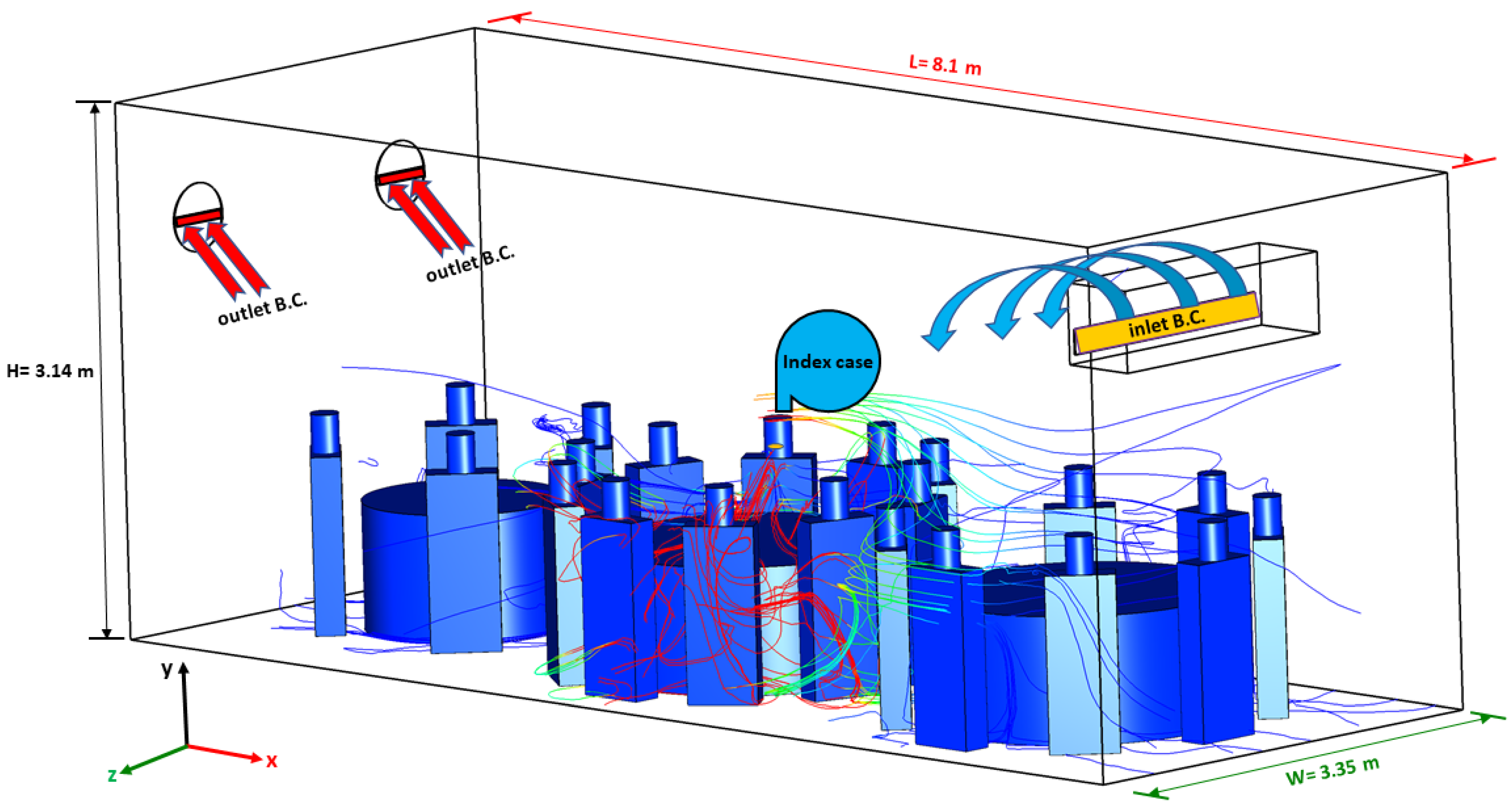
The present model simulates a real infection event of three unrelated families that occurred in a restaurant in Guangzhou, China, in January 2020. We labeled tables one, two, and three as table 1 (T1), table 2 (T2), and table 3 (T3), respectively and families sitting at these tables as family T1, family T2, and family T3, see Figure 1. The family members will be called customers. Figure 1 show the locations of the tables and the number of customers sitting around each table. During lunchtime, in addition to 8 staff members, there were 83 customers dining on the same floor of the five stories restaurant. One person in family B was already infected with COVID-19; however, he was asymptomatic when he dined with his family. After a few days, nine people sitting on tables T1, T2, and T3 were infected with COVID-19 even though some of them did not have direct contact with the sick person. The other customers sitting away from these three tables and the eight employees who were working on the floor at the time did not contract the virus. For the sake of simplicity, we labeled the customers as TXCYs (please, refer to Figure 1), where “X” represents the tables’ index and “Y” represents the customers’ number.

In the present model, human respiration activities, such as breathing, speaking, and sneezing within indoor environments, were simulated with CFD. CFD software AVL FIRE R2020 was used. Figure 2 illustrate the dimensions of the computational domain employed in the present model. The computational domain has dimensions of 3.35 m-width × 8.1 m-depth × 3.14 m-height. It was assumed that the ventilation of the computational domain was achieved through the air-conditioning unit in addition to the outlet area near the exhaust fans (please see Figure 2). The exhaust fans were not turned on, but the outlet area was open to the atmosphere.

A sinusoidal cycle was used to model the breathing mode. The infected individual was assumed to be breathing 10 times per minute, with a pulmonary rate of 6 L/min (3-s inhalation + 3-s exhalation) [6,22,24]. The current study treated air and droplets/particles as two different phases. Little is known about the aerosols produced by COVID-19 infected subjects. However, the size of SARS-CoV-2 (i.e., 60–160 nm) is very similar to the size of influenza viruses (80–100 nm) [2,4,5,10,34,35]. Researchers reported that the concentration of aerosol particles in human exhaled breath is ~10,000 particles per litre [17,35]. Therefore, one exhaled breath, which is between 0.3 and 0.75 L [36], could contain an order of 10³ droplets (≤1 µm) [37]. At the same time, a single sneeze can generate an order of 10⁴ or more droplets with a velocity up to 20 m s⁻¹ [5]. These aerosol particles are small enough to remain suspended in the air and pose a risk of airborne transmission. Different regions in the computational domain can be identified based on the presence of each droplet concentration. The average droplet size was assumed to be 1.0 µm [8,14,38,39]. To cater for the transient dynamic situation throughout the computational domain, the transport equations for both phases (i.e., gas and droplets) were solved.

A volume mesh was created based on an existing surface mesh using the FAME Hexa mesh generation technique. FAME Hexa is a smart tool for generating computational meshes. It generates meshes based on the discrete surface model, surface edges, and various settings. This technique was used to generate high-quality hexahedra grids. A dense mesh near the mouth was used, and then the sizes of the cells were gradually increased outward of the mouth region. This method reduces the total grid numbers for the current complex geometry, which helps to save computational time. Grid independence tests were carried out to select the grid size. Grid independence tests showed that there was no significant impact of the grid resolution on the results beyond 6,523,271 cell elements. Therefore, for all the subsequent simulations, the mesh consisting of 6,523,271 numerical elements was chosen.

2.3. Simulation and Numerical Procedures

Simulations were performed by means of the Finite Volume Method (FVM), using the commercial software AVL Fire. To discretize the flow equations, the first-order Euler scheme was used. The accuracy of this approach is reasonable in comparison with the second-order scheme, which is computationally expensive where it requires more simulation time and memory [40]. For accurate calculations of turbulent flows, the k-Ɛ turbulence model was utilized. The SIMPLE method was used to calculate the pressure [41]. Due to its higher stability, the GSTB was used in the current model as a linear solver for the solution of the main equations (i.e., momentum, continuity, turbulence, and scalar). Mass Residual was used in the present model to control the convergence. Here, the solution and the tolerance limit were set to 1 × 10⁻⁴. For all cases, the simulation time was 4500 s, and the time step size was 0.01 s.

2.4. Initial and Boundary Conditions

Boundary conditions specify the physical properties of the faces on the volume mesh. The boundary conditions have a significant impact on the accuracy of the flow computation and how well it represents the physical situation. The way the boundary conditions are applied also affects the convergence properties of the solution. The main boundary conditions used for this calculation setup are inlet boundary, outlet boundary, and wall boundary. Sine function was employed to prescribe the mass flow rate at the inlet, which fit quite well with the normal human breathing process [21]. At the outlet, an atmospheric pressure boundary condition was applied, as this is recommended when there are multiple outlets. For both phases (i.e., air and droplets), no-slip wall boundary conditions were applied. For the initial conditions in this work, the volume fraction of the gas phase was set to be one throughout the computational domain, while the volume fraction of the droplets was set to be zero. Figure 2 show the boundary conditions used in this work.

3. Results and Discussion

The present model simulates a real infection event of three unrelated families that occurred in a restaurant in Guangzhou, China, in January 2020. Lu, Gu, Li, Xu, Su, Lai, Zhou, Yu, Xu, and Yang [3] described in detail the epidemiological, clinical, laboratory, and genomic findings for this outbreak and all of the associated patients of the incident. We labeled the confirmed infected case (T2C1) from family T2 as an index case. The predicted results of the present model were compared with the reported data of the incident, and it was found that they were overall consistent; then, the model was used for further analysis. The present model examined five different scenarios, which are listed in

Table 1. The list of cases investigated in the present study.

	Ventilation Rate (Rate of Air Supplied from AC Units) per Person	Breathing and Talking	Sneezing
Case-1	0.9 L/s	Yes	No
Case-2	0.9 L/s	Yes	Yes
Case-3	1.35 L/s	Yes	No
Case-4	1.35 L/s	Yes	Yes
Case-5	Open-air conditions	Yes	No

.

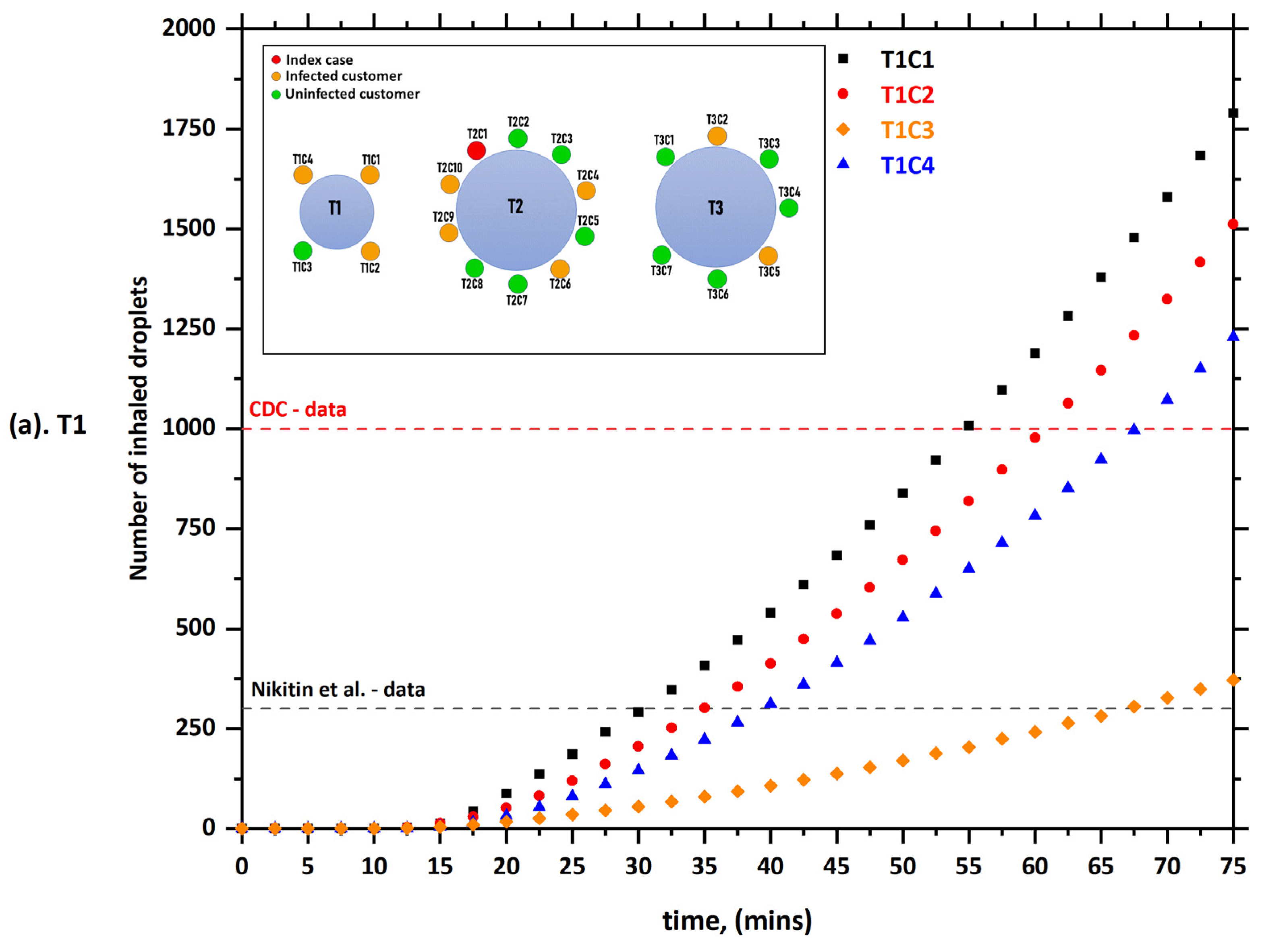
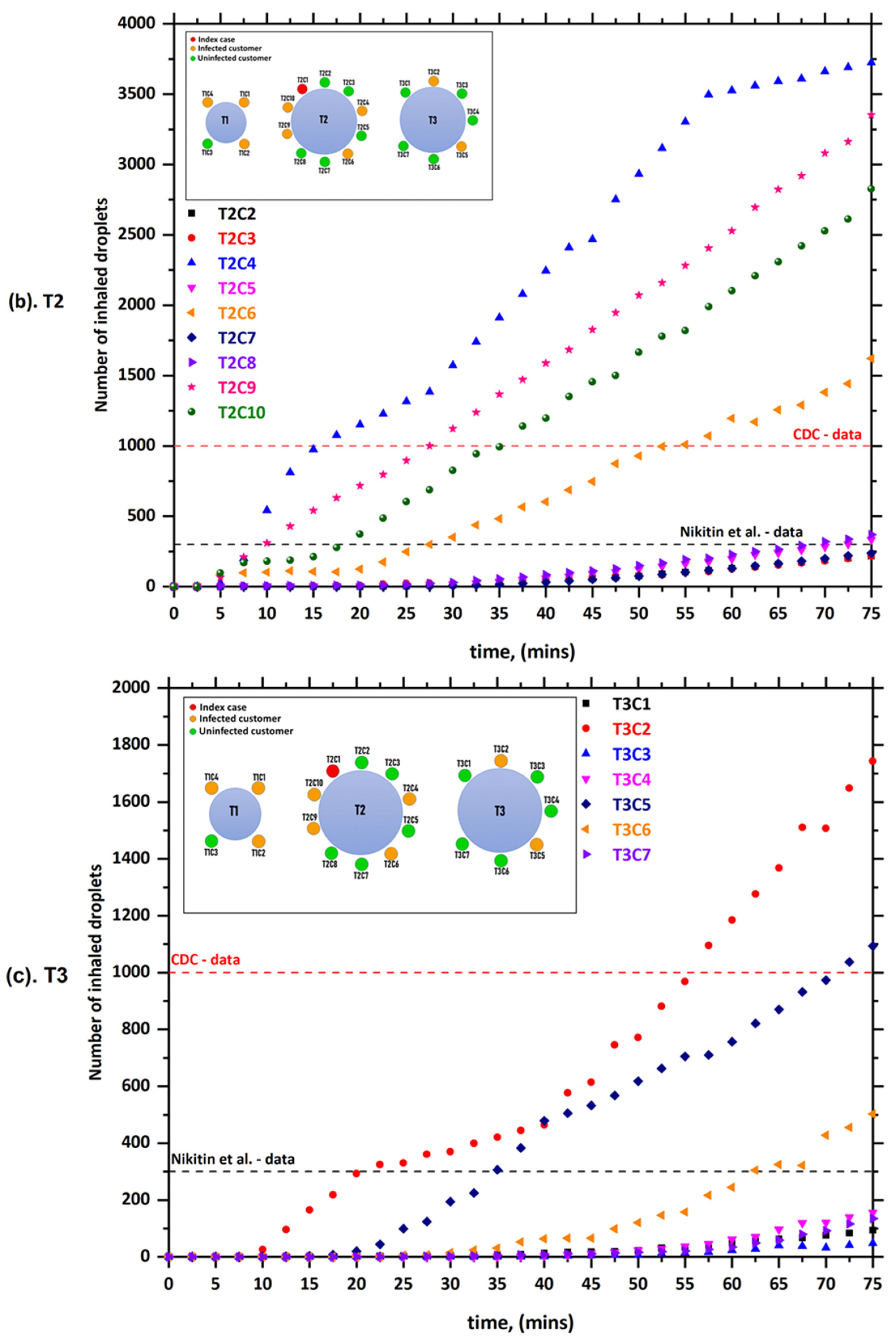
Figure 3 present the predicted results obtained from case-1 (i.e., (a) T1, (b) T2, and (c) T3). The number of inhaled aerosol droplets by healthy individuals through breathing and speaking is shown in Figure 3. It can be seen from the data in Figure 3a that three out of four customers (i.e., T1C1, T1C2, and T1C4) sitting at table 1 (T1) inhaled more than 300 aerosol droplets after only 30 min and more than 1000 droplets after 55 min. It also shows that two out of seven customers sitting at table 3 (T3) (i.e., T3C2 and T3C5) inhaled more than 300 aerosol droplets after only 20 min and more than 1000 droplets after 48 min. All these customers were reported to be infected with COVID-19 a few days after this incident. As we mentioned earlier, there was no direct contact between the index case (T2C1) and customers at the other tables (T1 and T3). In addition to that, the video records also reveal that the index case (T2C1) never turned his head toward T1 during lunch [3]. A possible explanation for this might be that the AC unit next to table ‘T3’ blew the air in the southward direction across all three tables; some of the air bounced off the wall back again in the direction of table 3 (T3) (will explain in detail later). This air movement led to the circulation of aerosol particles inside the computational domain, and this explains the infection of the customers sitting at tables T1 and T3. These results are consistent with those of Lu, Gu, Li, Xu, Su, Lai, Zhou, Yu, Xu, and Yang [3], who suggested that droplet transmission was the most likely primary cause of this outbreak. However, they stated that the outbreak could not be explained by only the droplet transmission. They argued that it is difficult to exclude the other possible scenario by which customers T1C2 and T1C4 were later infected outside the restaurant by patient T1C1 (i.e., the first member of family T1 to become infected with COVID-19). This is because the distance between the index case (T2C1) and customers at the other tables were all greater than 1 m [30]. Although the role of airborne transmission was first proposed by the Chinese National Health Commission (NHC) [42], there were no specific recommendations or data provided in this regard [30]. This study, however, provided strong evidence and confirmed the transmission of COVID-19 via airborne transmission. The results of the present model showed that the confirmed cases from other tables inhaled enough aerosol droplets to become infected with COVID-19. The results also show that the number of inhaled droplets increases with the increase of the duration people remain in the contaminated area. Figure 3 also show that people sharing the same table (T2C4, T2C6, T2C9, and T2C10) with the index case (T2C1) inhaled more droplets during a shorter time compared with other customers. For example, T2C4 inhaled more than 1000 droplets within less than 15 min (see, Figure 3). It is possible that these results are due to the fact the customers are sitting close to the index case (T2C1).

Figure 4 show the predicted results obtained by the current model of case-2. In case-2, it was assumed that the index case (T2C1) would sneeze a few times when t > 600 s. The main reason for focusing on sneezing in our model is the fact that sneezing happens to healthy people more frequently than coughing (episodes/day) every day [43]. Furthermore, it has the ability to spread infections and pathogens from asymptomatic carriers through the droplets that come out of the mouth during sneezing. The rate of air conditioning ventilation, in this case, was assumed to be similar to case-1 (0.9 L/s per person). Figure 4 show that there was a dramatic increase in the number of inhaled droplets by the other individuals in comparison with case-1. For example, T2C6 (i.e., the customer who was facing the index case (T2C1)) inhaled more than 300 droplets within less than 7 min and more than 1000 droplets within less than 12 min. These results were expected since a single sneeze can generate an order of 10⁴ or more droplets [5]. In addition, we can note from the results that sneezes have a profound effect on the aerodynamics of the computational domain, where the velocity of a sneeze is about 20 m s⁻¹ [5]. That means that the mixture of moist air and saliva that comes out of the mouth during sneezing will move straight and for a distance that may reach several meters.

The predicted droplet concentrations per cubic meter exhaled from the index case (T2C1) for different scenarios are presented in Figure 5, Figure 6, Figure 7, Figure 8 and Figure 9. From these figures we can see the contaminated cloud envelope in the computational domain where the color scale at the bottom of the figures illustrates the number of droplets per cubic meter.

Figure 5 show the predicted results of droplet concentrations per cubic meter exhaled from the index case (T2C1) for case-1. Figure 5 show that the stream of exhaled droplets from the index case (T2C1) collides with the air stream of the air-conditioning unit. The high momentum air-conditioning stream pushes the contaminated air in the southward direction across all three tables, and then some of the air will be bounced off the wall back again in the direction of table 3 (T3). This air movement led to the circulation of aerosol particles inside the computational domain, and this explains the infection of the customers sitting at tables T1 and T3. The red color refers to a higher concentration of contaminated droplets in that part of the computational domain, which leads to an increase in the possibility of inhaling more contaminated droplets and thus increases the risk of contracting the infection. In Figure 6, we presented the number of droplets per cubic meter from case-2. As mentioned earlier in Table 1, the boundary conditions for case-2 are similar to case-1; however, we assumed that the index case (T2C1) would start sneezing for few times at t = 600 s. It can be seen from the data in Figure 6 that the air stream of the air-conditioning unit had almost a similar influence on the concentration of contaminated droplets. However, the main difference between the two cases (i.e., case-1 and case-2) was that the concentration of contaminated droplets in the area in front of the index case (T2C1) was higher compared with case-1. These results are likely to be related to the fact the carrier fluid flow (i.e., exhaled air) had a maximum velocity near the mouth of the index (T2C1) case during the sneeze, and this will assist the cloud of contaminated droplets to follow a straight trajectory and travel far away from the location of the infected person. However, the velocity of the stream of contaminated droplets will drop gradually. This will cause an increase in the concentration of contaminated droplets in the area in front of the index case (T2C1). Furthermore, it is well known that the size of droplets that are produced from coughing or sneezing is much larger than the size of droplets produced through speaking or breathing, which means they will settle quickly [2,10,24,34,44]. However, these droplets from coughing or sneezing could travel for long distances and at high speeds, which may reach more than 8 m [2,34].

The effect of air conditioning ventilation conditions on the concentration of contaminated droplets is given in Figure 7, Figure 8 and Figure 9. Figure 7 illustrate the number of contaminated droplets per cubic meter exhaled from the index case (T2C1) through normal breathing and talking in 4500 s (case-3). In case-3, the air conditioning ventilation rate per person was increased by one and half times. Further, in this case (case-3), it was assumed the air would come out of the air conditioning unit at an angle of 45 degrees. Figure 7 show that the concentration of the contaminated droplets per cubic meter near table 3 (T3) were the lowest in comparison with other locations in the computational domain. These results are likely to be related to the influence of the air currents coming from the air-conditioning unit that was installed next to table 3 (T3). When the air current coming from the air-conditioning unit collides with the ground it will divide into two parts. A part of the flow travels toward the southward direction of the computational domain across table 2 (T2) and mixes with the contaminated droplets before bouncing off the wall and traveling back in the direction of table 3 (T3), where it is captured by a recirculation zone created by the air-conditioning unit.

The other part of the air current will return back to mix with the air current coming from the air-conditioning unit. The area around table 3 (T3) is protected by the air currents coming from the air conditioner, which acts as an air curtain reducing the number of contaminated droplets that will enter this area. Further, the increase in the air-conditioning airflow promotes turbulent transport. This will result in a complete disruption of the droplet cloud and an enhancement of its dispersion within the computational domain. These findings are consistent with data obtained by [45]. The number of contaminated droplets per cubic meter exhaled from the index case (T2C1) for case-4 in 4500 s is shown in Figure 8. The boundary conditions used in case-4 are similar to case-3. To examine the effect of air-conditioning on the dispersion of contaminated droplet within the computational domain, it was assumed that the index case (T2C1) would start sneezing for few times at t = 600 s. The concentration of contaminated droplets was higher near table 1 (T1) and part of table 2 (T2) as was found for case-3. However, the number of droplets per cubic meter was much higher, as expected, due to sneezing.

Figure 9 present the results obtained by the present model for case-5. To clearly evaluate the effect of the environmental surroundings on the distribution of the exhaled air stream from the index case (T2C1), in case-5, all the surrounding walls and roof ceiling were replaced under open-air atmosphere pressure boundary conditions. The order of tables and the number of customers sitting at each Table were similar to other cases. However, in this case, we assumed that the tables were placed outside the restaurant in the open air. The predicted results from case-5 are shown in Figure 9. Surprisingly, the contaminated droplets were concentrated on the second table (T2), where the index case (T2C1) was sitting. The predicted results suggested that the highest number of contaminated droplets would be concentrated around the people (i.e., T2C5, T2C6, T2C7, and T2C8) who were directly facing the index case (T2C1) (please, refer to Figure 9). This could be attributed to the fact the air exhaled from the index case (T2C1) will follow a straight path since there were no external air currents to influence or change this direction. It is worthy of mentioning that, although the distance between the index case (T2C1) and the people who were facing him was about 1.8 m, this distance was not enough to protect them from inhaling contaminated droplets. In general, the dispersion of contaminated droplets in case-5 was less compared to the other cases. In the absence of the air-conditioning, the droplets were only under the effect of the gravitational force grounding them on the floor [45].

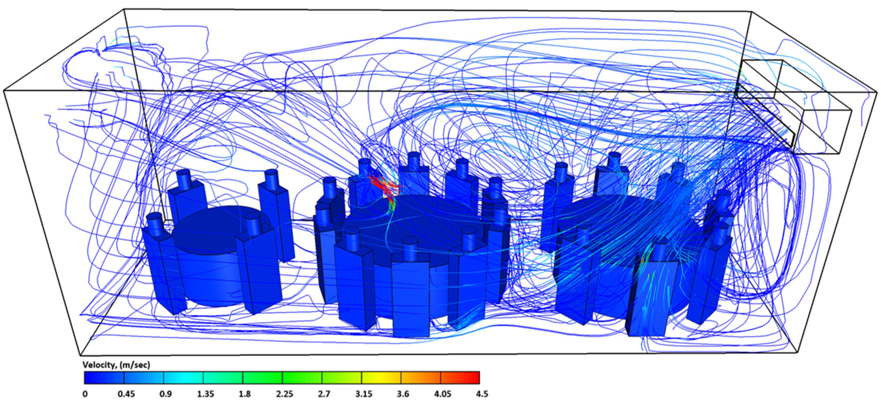
Flow velocity streamlines of case-1, case-2, case-3, case-4, and case-5 are shown in Figure 10, Figure 11, Figure 12, Figure 13 and Figure 14. As can be seen from Figure 10, Figure 11, Figure 12 and Figure 13, the flow circulation in the computational domain was dominated by the air conditioning. However, sneezing had a significant influence on the streamlined velocity of the exhaled air and thus the concentrations of the contaminated droplets (please, see Figure 11 and Figure 13). For case-5 (outdoor conditions), we can see that the airflow inside the computational domain was completely dominated by cyclic breathing and talking; Figure 14. The air conditioning system created a state of air circulation inside the computational domain, which had a significant effect on the aerodynamics of the droplets and their settling velocities. These observations support what was explained in the previous Figure on the effect of air conditioning units on the concentration of inhaled droplets by healthy individuals.

The predicted contaminated droplet velocities at the early period of ejection from a human sneeze are illustrated in Figure 15 and Figure 16. It was observed that the exhaled air velocity was at the maximum value near the mouth of the index case (T2C1), and drops traveled gradually downstream. Due to the high velocity of the sneeze, the contaminated droplets followed a straight trajectory, especially in the absence of an air-conditioning system. At longer distances, the cloud of the contaminated droplets will settle at different rates under the effect of gravity. As explained earlier, the high momentum of the exhaled air during sneezing will cause more disturbance within the flow domain which will have a significant effect on the distribution of the contaminated droplets.

4. Summary and Conclusions

In this study, Computational Fluid Dynamics (CFD) was utilized to investigate the aerosol transport of SARS-CoV-2 in a restaurant environment. The developed CFD model was used to accurately predict the time duration to becoming infected while sharing an indoor space with a patient with COVID-19 or a similar virus. The present CFD model predicts the number of aerosol droplets inhaled by every individual inside an enclosed space such as a restaurant through breathing, speaking, and sneezing. This type of prediction by the present model is useful for the effective prevention of infectious airborne diseases such as SARS-CoV-2 by identifying the movement of the droplets in public places such as a restaurant and predicting the spread of disease. The main findings of the present work can be summarized as follows:

• In total, 10 min is all that you need to become infected with COVID-19 when sharing a table with a coronavirus patient;
• The complex patterns of airflow caused by ventilation systems help keep aerosol droplets suspended in the air for a longer time;
• Although changing the ventilation rate will improve the quality of air within closed spaces, it will not be enough to protect people from COVID-19;
• Within an indoor environment, 1.8 m between tables (1.8 m is the CDC’s recommendation) is not enough distance to safeguard individuals in a restaurant or similar public places;
• Eating outdoors, in addition to increasing the spaces between tables, will reduce the risk of infection.

References

- Australia Government Department of Health. What You Need to Know about Coronavirus (COVID-19). Available online: https://www.health.gov.au/news/health-alerts/novel-coronavirus-2019-ncov-health-alert/what-you-need-to-know-about-coronavirus-covid-19 (accessed on 6 April 2021).
- World Health Organization (WHO). Coronavirus Disease (COVID-19) Pandemic. Available online: https://www.who.int/emergencies/diseases/novel-coronavirus-2019 (accessed on 25 May 2021).
- Lu, J.; Gu, J.; Li, K.; Xu, C.; Su, W.; Lai, Z.; Zhou, D.; Yu, C.; Xu, B.; Yang, Z. COVID-19 Outbreak Associated with Air Conditioning in Restaurant, Guangzhou, China, 2020. Emerg. Infect. Dis. 2020, 26, 1628–1631. [Google Scholar] [CrossRef] [PubMed]
- Scheuch, G. Breathing Is Enough: For the Spread of Influenza Virus and SARS-CoV-2 by Breathing Only. J. Aerosol Med. Pulm. Drug. Deliv. 2020, 33, 230–234. [Google Scholar] [CrossRef] [PubMed]
- Mittal, R.; Ni, R.; Seo, J.-H. The flow physics of COVID-19. J. Fluid Mech. 2020, 894, F2. [Google Scholar] [CrossRef]
- Hui, D.S.; Chow, B.K.; Lo, T.; Tsang, O.T.Y.; Ko, F.W.; Ng, S.S.; Gin, T.; Chan, M.T.V. Exhaled air dispersion during high-flow nasal cannula therapy versus CPAP via different masks. Eur. Respir. J. 2019, 53, 1802339. [Google Scholar] [CrossRef] [PubMed]
- Longo, L. COVID-19, What It Is and How It Behaves. Available online: https://www.eni.com/en-IT/scientific-research/covid-19-what-how-behaves.html (accessed on 29 April 2021).
- Anderson, E.L.; Turnham, P.; Griffin, J.R.; Clarke, C.C. Consideration of the Aerosol Transmission for COVID-19 and Public Health. Risk Anal. 2020, 40, 902–907. [Google Scholar] [CrossRef] [PubMed]
- Asadi, S.; Bouvier, N.; Wexler, A.S.; Ristenpart, W.D. The coronavirus pandemic and aerosols: Does COVID-19 transmit via expiratory particles? Aerosol Sci. Technol. 2020, 54, 635–638. [Google Scholar] [CrossRef] [PubMed] [Green Version]
- Morawska, L.; Cao, J. Airborne transmission of SARS-CoV-2: The world should face the reality. Environ. Int. 2020, 139, 105730. [Google Scholar] [CrossRef] [PubMed]
- Yao, M.; Zhang, L.; Ma, J.; Zhou, L. On airborne transmission and control of SARS-Cov-2. Sci. Total Environ. 2020, 731, 139178. [Google Scholar] [CrossRef]
- Li, Y.; Qian, H.; Hang, J.; Chen, X.; Hong, L.; Liang, P.; Li, J.; Xiao, S.; Wei, J.; Liu, L.; et al. Evidence for probable aerosol transmission of SARS-CoV-2 in a poorly ventilated restaurant. medRxiv 2020. [Google Scholar] [CrossRef] [Green Version]
- Duguid, J.P. The size and the duration of air-carriage of respiratory droplets and droplet-nuclei. J. Hyg. 1946, 44, 471–479. [Google Scholar] [CrossRef] [Green Version]
- Fairchild, C.; Stampfer, J. Particle concentration in exhaled breath. Am. Ind. Hyg. Assoc. J. 1987, 48, 948–949. [Google Scholar] [CrossRef] [PubMed]
- Papineni, R.S.; Rosenthal, F.S. The size distribution of droplets in the exhaled breath of healthy human subjects. J. Aerosol Med. 1997, 10, 105–116. [Google Scholar] [CrossRef] [PubMed]
- Edwards, D.A.; Man, J.C.; Brand, P.; Katstra, J.P.; Sommerer, K.; Stone, H.A.; Nardell, E.; Scheuch, G. Inhaling to mitigate exhaled bioaerosols. Proc. Natl. Acad. Sci. USA 2004, 101, 17383–17388. [Google Scholar] [CrossRef] [PubMed] [Green Version]
- Fabian, P.; McDevitt, J.J.; DeHaan, W.H.; Fung, R.O.; Cowling, B.J.; Chan, K.H.; Leung, G.M.; Milton, D.K. Influenza virus in human exhaled breath: An observational study. PLoS ONE 2008, 3, e2691. [Google Scholar] [CrossRef] [PubMed] [Green Version]
- Chao, C.Y.H.; Wan, M.P.; Morawska, L.; Johnson, G.R.; Ristovski, Z.; Hargreaves, M.; Mengersen, K.; Corbett, S.; Li, Y.; Xie, X. Characterization of expiration air jets and droplet size distributions immediately at the mouth opening. J. Aerosol Sci. 2009, 40, 122–133. [Google Scholar] [CrossRef] [Green Version]
- Morawska, L.; Johnson, G.; Ristovski, Z.; Hargreaves, M.; Mengersen, K.; Corbett, S.; Chao, C.Y.H.; Li, Y.; Katoshevski, D. Size distribution and sites of origin of droplets expelled from the human respiratory tract during expiratory activities. J. Aerosol Sci. 2009, 40, 256–269. [Google Scholar] [CrossRef] [Green Version]
- Han, Z.Y.; Weng, W.G.; Huang, Q.Y. Characterizations of particle size distribution of the droplets exhaled by sneeze. J. R. Soc. Interface 2013, 10, 20130560. [Google Scholar] [CrossRef]
- Leonard, S.; Strasser, W.; Whittle, J.S.; Volakis, L.I.; DeBellis, R.J.; Prichard, R.; Atwood, C.W., Jr.; Dungan, G.C., II. Reducing aerosol dispersion by High Flow Therapy in COVID-19: High Resolution Computational Fluid Dynamics Simulations of Particle Behavior during High Velocity Nasal Insufflation with a Simple Surgical Mask. J. Am. Coll. Emerg. Phys. Open 2020, 1, 578–591. [Google Scholar] [CrossRef]
- Riediker, M.; Tsai, D.H. Estimation of Viral Aerosol Emissions From Simulated Individuals With Asymptomatic to Moderate Coronavirus Disease 2019. JAMA Netw. Open 2020, 3, e2013807. [Google Scholar] [CrossRef]
- Van Doremalen, N.; Bushmaker, T.; Morris, D.H.; Holbrook, M.G.; Gamble, A.; Williamson, B.N.; Tamin, A.; Harcourt, J.L.; Thornburg, N.J.; Gerber, S.I.; et al. Aerosol and Surface Stability of SARS-CoV-2 as Compared with SARS-CoV-1. N. Engl. J. Med. 2020, 382, 1564–1567. [Google Scholar] [CrossRef]
- Vuorinen, V.; Aarnio, M.; Alava, M.; Alopaeus, V.; Atanasova, N.; Auvinen, M.; Balasubramanian, N.; Bordbar, H.; Erasto, P.; Grande, R.; et al. Modelling aerosol transport and virus exposure with numerical simulations in relation to SARS-CoV-2 transmission by inhalation indoors. Saf. Sci. 2020, 130, 104866. [Google Scholar] [CrossRef] [PubMed]
- Liu, H.; He, S.; Shen, L.; Hong, J. Simulation-Based Study on the COVID-19 Airborne Transmission in a Restaurant. medRxiv 2020. [Google Scholar] [CrossRef]
- Wang, W.; Wang, F.; Lai, D.; Chen, Q. Evaluation of SARS-COV-2 transmission and infection in airliner cabins. Indoor Air 2022, 32, e12979. [Google Scholar] [CrossRef] [PubMed]
- Bhattacharyya, S.; Dey, K.; Paul, A.R.; Biswas, R. A novel CFD analysis to minimize the spread of COVID-19 virus in hospital isolation room. Chaos Solitons Fractals 2020, 139, 110294. [Google Scholar] [CrossRef] [PubMed]
- Feng, Y.; Marchal, T.; Sperry, T.; Yi, H. Influence of wind and relative humidity on the social distancing effectiveness to prevent COVID-19 airborne transmission: A numerical study. J. Aerosol Sci. 2020, 147, 105585. [Google Scholar] [CrossRef]
- Abuhegazy, M.; Talaat, K.; Anderoglu, O.; Poroseva, S.V. Numerical investigation of aerosol transport in a classroom with relevance to COVID-19. Phys. Fluids 2020, 32, 103311. [Google Scholar] [CrossRef]
- Li, Y.; Qian, H.; Hang, J.; Chen, X.; Cheng, P.; Ling, H.; Wang, S.; Liang, P.; Li, J.; Xiao, S.; et al. Probable airborne transmission of SARS-CoV-2 in a poorly ventilated restaurant. Build. Environ. 2021, 196, 107788. [Google Scholar] [CrossRef]
- Wang, Z.; Galea, E.R.; Grandison, A.; Ewer, J.; Jia, F. A coupled Computational Fluid Dynamics and Wells-Riley model to predict COVID-19 infection probability for passengers on long-distance trains. Saf. Sci. 2022, 147, 105572. [Google Scholar] [CrossRef]
- AVL FIRE Software Documentation; 2020 R1; AVL List GmbH: Graz, Austria, 2021.
- Concept Smoke System. Particle Size & Settling Velocities. Available online: http://www.smokemachines.com/settling-velocities-particle-size.aspx (accessed on 17 June 2021).
- Centers for Disease Control and Prevention (CDC). About COVID-19. Available online: https://www.cdc.gov/ (accessed on 21 March 2021).
- Nikitin, N.; Petrova, E.; Trifonova, E.; Karpova, O. Influenza virus aerosols in the air and their infectiousness. Adv. Virol. 2014, 2014, 859090. [Google Scholar] [CrossRef] [Green Version]
- Ai, Z.T.; Melikov, A.K. Airborne spread of expiratory droplet nuclei between the occupants of indoor environments: A review. Indoor Air 2018, 28, 500–524. [Google Scholar] [CrossRef]
- Yan, J.; Grantham, M.; Pantelic, J.; Bueno de Mesquita, P.J.; Albert, B.; Liu, F.; Ehrman, S.; Milton, D.K.; Consortium, E. Infectious virus in exhaled breath of symptomatic seasonal influenza cases from a college community. Proc. Natl. Acad. Sci. USA 2018, 115, 1081–1086. [Google Scholar] [CrossRef] [PubMed] [Green Version]
- Asadi, S.; Wexler, A.S.; Cappa, C.D.; Barreda, S.; Bouvier, N.M.; Ristenpart, W.D. Aerosol emission and superemission during human speech increase with voice loudness. Sci. Rep. 2019, 9, 2348. [Google Scholar] [CrossRef] [PubMed] [Green Version]
- Yip, L.; Finn, M.; Granados, A.; Prost, K.; McGeer, A.; Gubbay, J.B.; Scott, J.; Mubareka, S. Influenza virus RNA recovered from droplets and droplet nuclei emitted by adults in an acute care setting. J. Occup. Environ. Hyg. 2019, 16, 341–348. [Google Scholar] [CrossRef] [PubMed]
- Sarhan, A.R.; Naser, J.; Brooks, G. Bubbly flow with particle attachment and detachment—A multi-phase CFD study. Sep. Sci. Technol. 2017, 53, 181–197. [Google Scholar] [CrossRef]
- Patankar, S.V.; Spalding, D.B. Paper 5—A Calculation Procedure for Heat, Mass and Momentum Transfer in Three-Dimensional Parabolic Flows. In Numerical Prediction of Flow, Heat Transfer, Turbulence and Combustion; Patankar, S.V., Pollard, A., Singhal, A.K., Vanka, S.P., Eds.; Pergamon: Oxford, UK, 1983; pp. 54–73. [Google Scholar]
- Chinese National Health Commission (NHC). Available online: http://en.nhc.gov.cn/ (accessed on 8 March 2022).
- Busco, G.; Yang, S.R.; Seo, J.; Hassan, Y.A. Sneezing and asymptomatic virus transmission. Phys Fluids 2020, 32, 073309. [Google Scholar] [CrossRef] [PubMed]
- Bhagat, R.K.; Davies Wykes, M.S.; Dalziel, S.B.; Linden, P.F. Effects of ventilation on the indoor spread of COVID-19. J. Fluid Mech. 2020, 903, F1. [Google Scholar] [CrossRef]
- Borro, L.; Mazzei, L.; Raponi, M.; Piscitelli, P.; Miani, A.; Secinaro, A. The role of air conditioning in the diffusion of Sars-CoV-2 in indoor environments: A first computational fluid dynamic model, based on investigations performed at the Vatican State Children’s hospital. Environ. Res. 2021, 193, 110343. [Google Scholar] [CrossRef]
Figure 1.
Sketch of locations of tables and the number of customers sitting around each table.
Figure 2.
The dimensions of the computational domain used in the present model.
Figure 3.
The number of inhaled droplets/particles by healthy individuals in a restaurant setting—case-1; (a) T1: table 1, (b) T2: table 2, and (c) T3: table 3 [35].
Figure 4.
The number of inhaled droplets/particles by healthy individuals in a restaurant setting—case-2; (a) T1: table 1, (b) T2: table 2, and (c) T3: table 3 [35].