
Multifidelity Analysis of a Solo Propeller: Entropy Rise Using Vorticity Dynamics and Kinetic Energy Dissipation

Department of Aerospace Engineering, University of Cincinnati, Cincinnati, OH 45221, USA
*
Author to whom correspondence should be addressed.
Fluids 2022, 7(5), 177; https://0-doi-org.brum.beds.ac.uk/10.3390/fluids7050177
Submission received: 1 April 2022
/
Revised: 5 May 2022
/
Accepted: 17 May 2022
/
Published: 20 May 2022
Abstract
:Propellers for electric aviation are used in solo- and multirotor applications. Multifidelity analysis with reduced cycle time is crucial to explore several designs for energy minimization and range maximization. A low-fidelity design tool, py_BEM, is developed for design and analysis of a reverse-engineered solo 2-bladed propeller using blade-element momentum theory with physics enhancements including local Reynolds number effect, boundary-layer rotation, airfoil polar at large AoAs and stall delay. Spanwise properties from py_BEM are converted into 3D blade geometry using T-Blade3. S809 and NACA airfoil polar are utilized, obtained by XFOIL. Lift, drag, performance losses, wake analysis, comparison of 3D steady CFD with low fidelity tool, kinetic energy dissipation, entropy and exergy through irreversibility are analyzed. Spanwise thrust and torque comparison between low and high fidelity reveals the effect of blade rotation on the polar. Vorticity dynamics and boundary-vorticity flux methods describe the onset of flow separation and entropy rise. Various components of drag and loss are accounted. The entropy rise in the boundary layer and downstream propagation and mixing out with freestream are demonstrated qualitatively. Irreversibility is accounted downstream of the rotor using the second-law approach to understand the quality of available energy. The performance metrics are within 5% error for both fidelities.
1. Introduction
Urban air mobility, drones and propeller-driven aircrafts are taking advantage of electric propulsion technology to invest in traditional and nontraditional vehicles [1]. The design of an optimum propeller is the key enabler to maximize range, reduce noise and be part of a robustly distributed propulsion system. Reduced cycle time is necessary to investigate several designs with varying constraints from multiple domains [2]. While low-fidelity tools with well-tweaked accuracy are better suited in the initial design phase [3], a more detailed analysis is necessary to understand the flow physics obtained by high-fidelity tools [4]. Off-design analysis is faster in low fidelity to examine the working range of designs instead of taking several days for high-fidelity analysis, delaying the development phase [5,6]. A low-fidelity tool based on blade-element momentum theory, takes few minutes to run, whereas 3D/4D CFD run times are in the order of several hours/days depending on the mesh quality and computational resources. Low-fidelity tools provide a good initial design that can be converted into 3D geometry for high-fidelity analysis [7,8]. Capturing physics at this level is crucial in obtaining a design closer to a realistic shape and ensuring a convergence of solution [9,10,11,12]. Tools which incorporate the effect of the Reynolds number spanwise, aerodynamic loading near- and post-stall and rotational effect on lift-and-drag polars are necessary at low fidelity. Some designs take advantage of exit swirl using contrarotating systems [13,14]. Numerical and experimental analysis of the propeller blades in isolation or with the aircraft provides a detailed accounting of the energy coefficients [15], boundary-layer transition and separation, which was historically mainly conducted using experiments [16,17]. Wake interaction [18], performance losses and entropy generated [19] and near- and far-field vortex behavior [20,21] are important to understand while designing a novel propulsion system. Flow physics interpretation, kinetic energy dissipated downstream [22,23], drag prediction [24] and lift distribution on the rotor blades need to be investigated in multifidelity to improve the quality of on-board energy consumption. Comparison with low-fidelity results demonstrates the assumptions at each level and educates the designer to enhance the low-fidelity tools to reduce cycle time. Exergy analysis and power-balance methods demonstrate the mechanics of available energy split into various forms, dissipation downstream as wakes and assesses the total performance [25,26,27].
Some of the recent work on comparing blade-element methods against RANS simulations and test data has been performed by Bergmann et al. [28] who showed the strength of the BET tools compared to RANS simulations with 15–20% overprediction error. Jin et al. [29] improved the fixed-point iteration algorithm popularly used in BEMT-based tools to make it robust with improved computational efficiency. Ning [30] improved the convergence of BEMT solutions using a single residual form and gradient-based design optimization. Hoyos et al. [31] optimized an aircraft propeller using a convergence-improved BEMT tool and validated it with OpenFOAM CFD results. They also incorporated a structural model to understand the impact of centrifugal forces. Treuren et al. [32] developed a tool, CLPROP, using BEMT and minimum induced loss by unloading the thrust produced at the tip of the propeller, which significantly reduced the tip vortex formation, rendering less required torque. In the broader context, there have been other design methods for unducted rotors. Naung et al. [33] proposed a frequency-domain method to numerically study the aerodynamic performance of a vibrating wind turbine, and Hasan et al. [34] demonstrated the effects of rotation on unsteady fluid flow in a rotating curved square duct with a small curvature.
This paper aims to capture flow physics and energy conversion by propellers at low and high fidelities and is organized as follows: A brief methodology for the low-fidelity tool is described for a reverse-engineered representative propeller blade [35,36] and airfoil properties obtained are discussed. A tool based on BEMT is developed with physics enhancements including local Reynolds number effect, 3D rotational corrections, stall delay model, airfoil polar at larger AoAs, integration to a 3D geometry generator, off-design model calculation, axial and tangential momentum loss and exergetic efficiency using the second law. The results of low-fidelity analysis are converted into 3D geometry, and 3D steady CFD analysis setup is described. The Results section compares the two fidelities and provides a detailed account for momentum transport, swirl, vorticity and kinetic energy dissipation downstream of the rotor with a rigorous domain and mesh-dependency study. Different forms of drag are also accounted. The boundary-vorticity flux method is utilized to post-process flow and explain the onset of flow separation on the blade, skin friction and vorticity created in the boundary layer. The mechanism of entropy increase, starting from the boundary layer, dissipation into the near field and as wake propagation in the far field is investigated. Exergy and irreversibility analysis quantify the amount of available energy utilized by the rotor.
2. Methodology
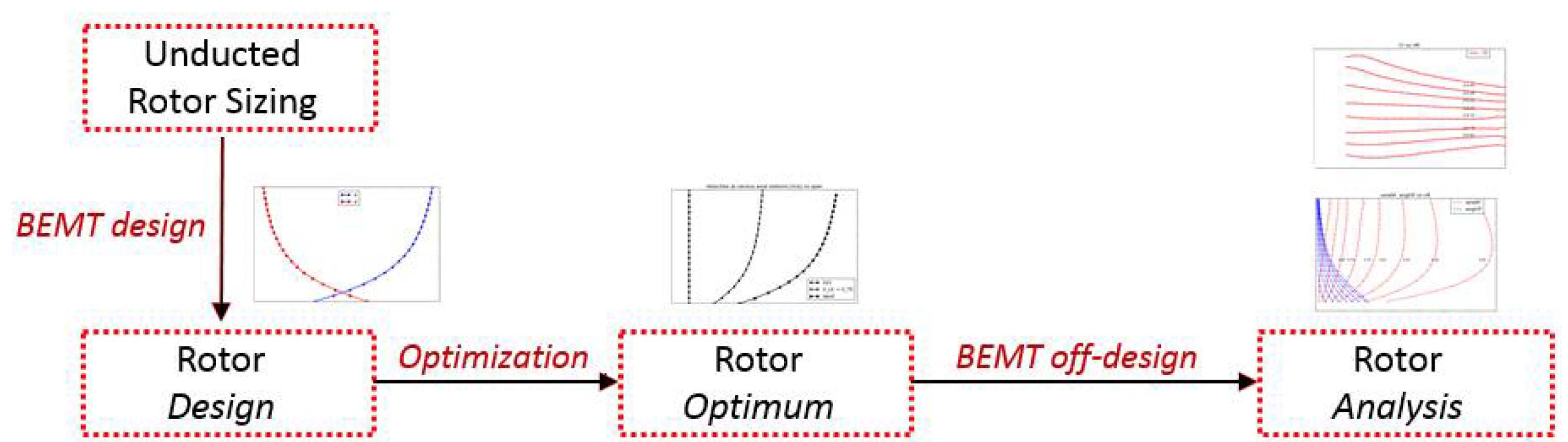
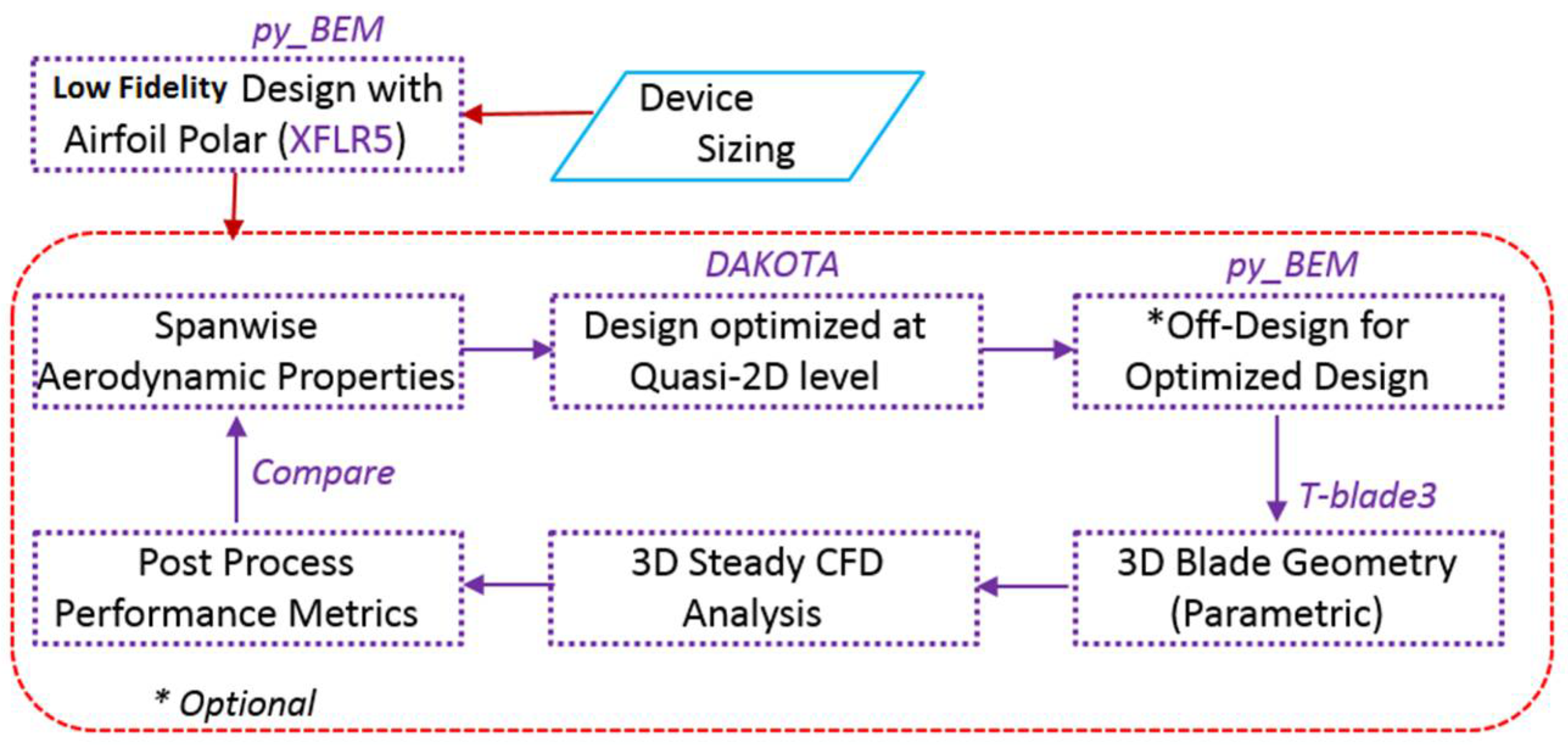
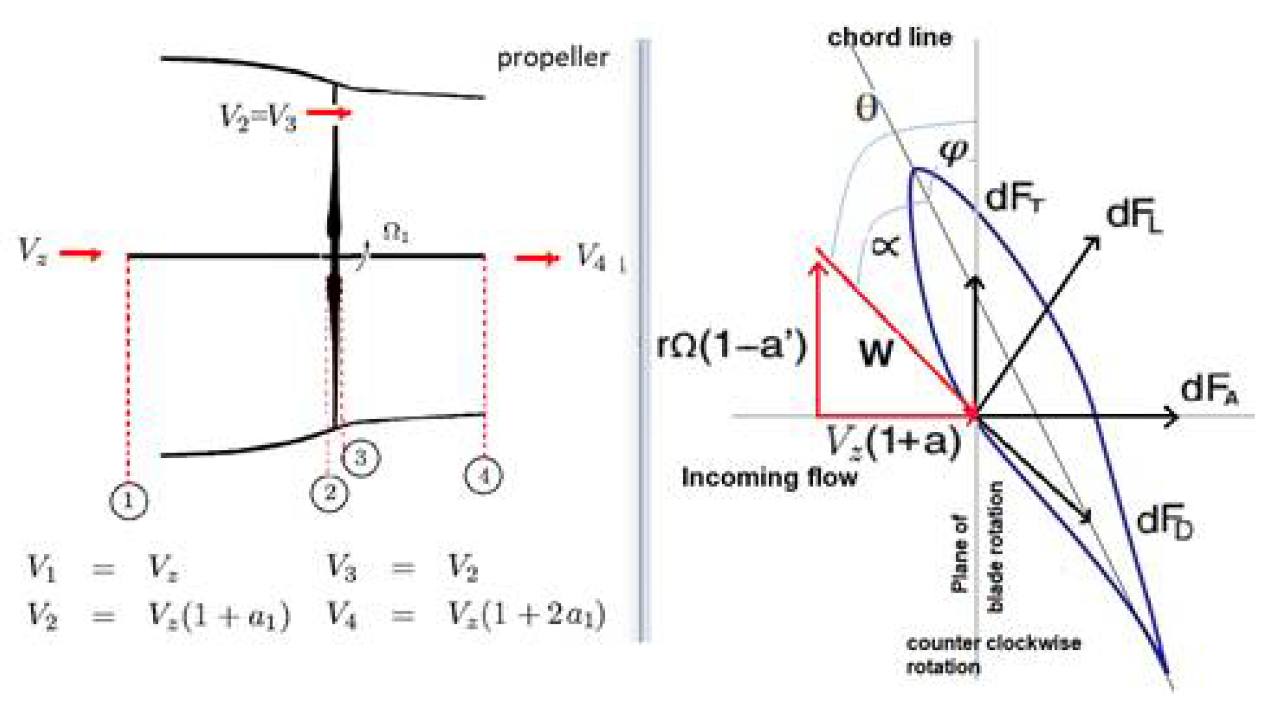
A general low-fidelity tool, py_BEM, based on blade-element momentum theory, is developed to design propellers, wind and hydrokinetic turbines, which includes the spanwise variation of REYN and airfoil polar [37]. A 3D blade geometry is constructed from the results of py_BEM and used in a high-fidelity CFD analysis loop. A two-bladed propeller rotor is designed, and off-design metrics are calculated, as shown in Figure 1. Figure 2 shows the complete process of multifidelity analysis. Blade-momentum theory considers the linear momentum conservation principle and utilizes Bernoulli’s principle across a rotating disk. Velocity increases at various axial locations due to the flow contraction, and spanwise thrust and torque are calculated, as shown in Figure 3. It assumes the flow to be one-dimensional, incompressible, steady, inviscid, irrotational and with no swirl in the wake. Four points of interest are upstream of the rotor, near the leading edge, trailing edge and far downstream of the rotor. Blade-element theory is used to design the rotor accounting for airfoil characteristics spanwise. It assumes that the blade is divided into several radial 2D sections for aerodynamic loading without any radial flow between them.
Fractional increase in axial velocity between free stream and rotor plane is defined as the axial induction factor a. If wake rotation is considered, a small angular velocity is imparted to the flow stream, and fractional change of angular velocity across the rotating disk is defined as angular induction factor, a’. The elemental torques from both theories are equated to obtain an expression for a’. The geometric relation of the velocity triangles from blade-element theory is used to get another expression for a’. These two expressions are equated as they are identical, to obtain an expression for the axial induction factor a in terms of the flow angle ϕ defined as g(ϕ). Now, the elemental thrusts from both theories are equated to obtain an equation entirely as a function of ϕ. This f(ϕ, g(ϕ)) = 0 is solved using the bisection method for a unique root between the prescribed bounds for solo and contrarotating configurations.
The tool, py_BEM, connects low- and high-fidelity domains. The spanwise variation of the airfoil properties become inputs for a parametric 3D blade-geometry generator to create a high-fidelity blade for CFD analysis, and the tool is part of an optimization framework for designing blades with maximum thrust or torque as required [37]. Three-dimensional CFD analysis is performed on the blade with rigorous grid and domain dependency to investigate their effect on performance. Comparisons between low- and high-fidelity results reveal the assumptions inherent in each fidelity. Wake analysis, vorticity dynamics, momentum and kinetic energy transport are explained and connected to the entropy generated by the rotor. Boundary-vorticity flux-driven analysis reveals the on-wall signature of flow separation and flow physics associated with vorticity propagation. Drag created by the rotor is also investigated, which distinguishes the lift-induced drag and pressure drag with emphasis on skin-friction-coefficient behavior due to mesh density, domain size and inclusion of turbulence-transition schemes in 3D RANS steady solution.
Input data are utilized to calculate the induction factors, spanwise blade-geometry properties and aerodynamic loads in terms of elemental thrust and torque on each blade element radially, which is looped through the entire blade span. As outputs, py_BEM creates design summary, performance coefficients, losses, off-design analysis input data and also a 3D blade-shape input file. Input data are categorized into types of fluid, device, configuration, airfoil, inflow and airfoil polar-enhancement flags [37]. Several types of losses are calculated in py_BEM, such as tip loss using Prandtl’s loss model, axial and tangential momentum loss, exergy and entropy-based loss. A bisection method [37] is incorporated to solve the nonlinear relationship between the induction factors and the flow angle established in Equations (1)–(4) due to its simplicity and robustness. It is a root finder for the function with limits on the flow angles based on propeller physics. Inputs are the flow angle interval, continuous function and values at the limits. The iterative solver calculates the midpoint of the flow angle interval, evaluates the function at this midpoint, and if the function crosses zero then the midpoint is the value of flow angle, otherwise it repeats this process.
2.1. Airfoil Properties
Airfoil properties are essential components in predicting the performance of an unducted rotor using low-fidelity approaches such as BEMT. An airfoil polar can be obtained from several methods: experimental results, XFOIL/RFOIL runs and 2D/3D CFD analysis, and it is very difficult to obtain similar values. The inlet turbulence intensity between experiments and simulations needs to be matched very well. Lift-and-drag properties of an airfoil depend on Reynolds number and angle of attack. The angle between the airfoil chord axis and the relative velocity Vrel is called angle of attack. In 2D, AoA is defined geometrically using the chord axis and the far upstream velocity, but it is very difficult to define AoA in 3D due to three-dimensional effects around the rotor. The definition of relative velocity is difficult due to the bound circulation influence, and this affects the AoA. Hence, the induced velocities to determine AoA should come from all vorticities other which are different from bound vorticity of the current airfoil section. There are other components of AoA, such as induced AoA and effective AoA due to the downwash, which need to be taken into account for accuracy. A vast library of NACA4415 airfoil lift-and-drag properties as a function of AoA (−10.00 to 10.00 degrees) for a wide range of Reynolds number (0.01 × 10⁶–0.99 × 10⁶) is created using XFLR5/XFOIL [38]. This library is used as a look-up table to obtain airfoil properties spanwise at the corresponding Reynolds number, including thrust and torque values calculated spanwise in py_BEM.
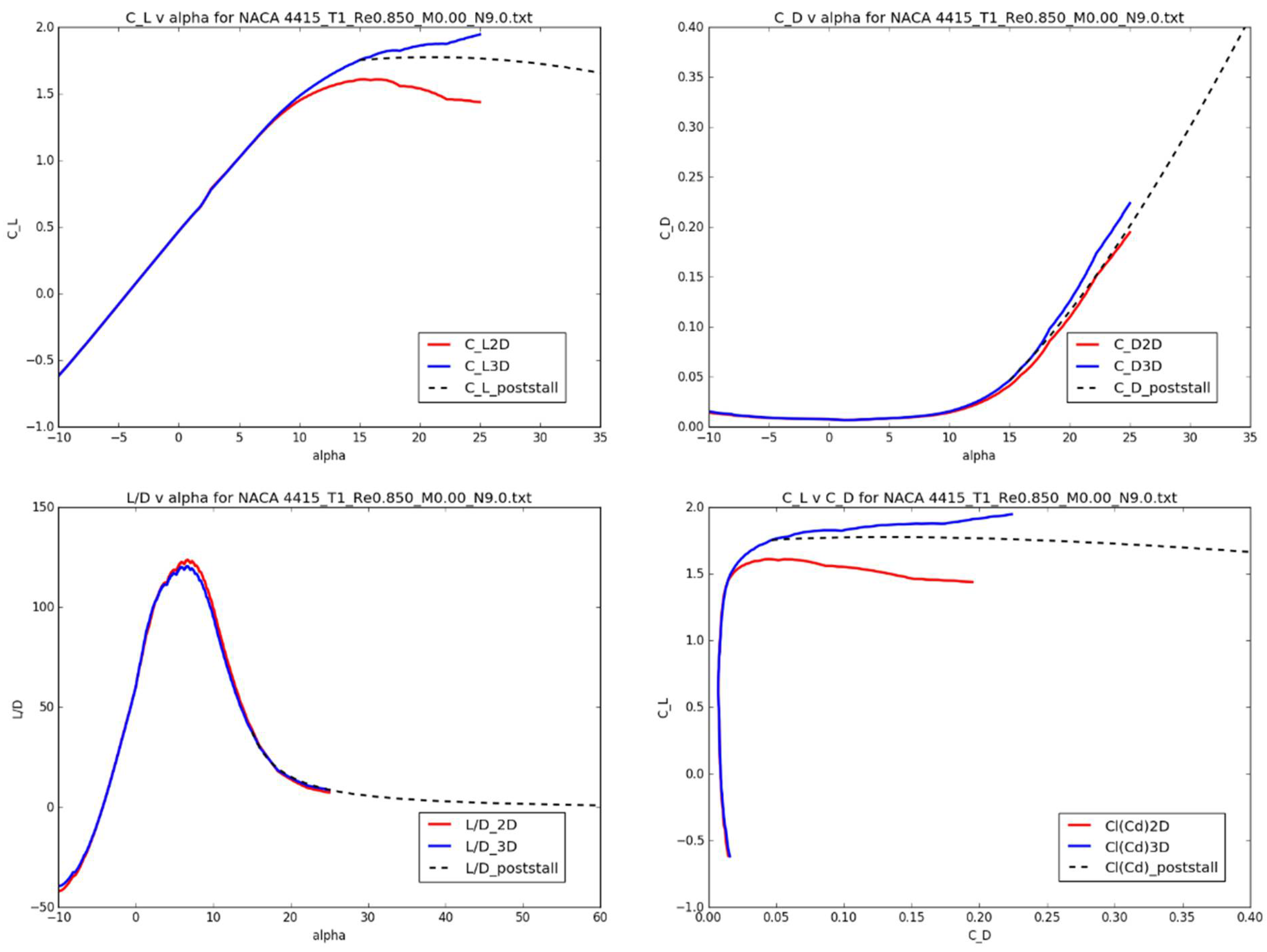
Polars obtained from the above methods do not include rotational effects. 3D rotational corrections are added to 2D polars using the Du and Selig model [39]. Airfoil polar tables must be extended to a larger range of AoA beyond the stall angle. Flow separation on the airfoil suction side in the stall regime makes the lift-and-drag measurements complicated, using pressure transducers and wake rakes. Numerically, stalled airfoil simulations use more complicated schemes and computational resources for accurate prediction of lift-and-drag coefficients at higher angles of attack. The extrapolation of polars using flat-plate theory at higher AoA is a valid solution for such situations. It is based on the similarity between the airfoil and the flat plate at such AoA. Viterna [40] came up with an empirical method to calculate polar at higher AoA, and this model is used in py_BEM. An airfoil polar at higher AoA is essential to obtain a successful convergence with the BEMT-based tool. Figure 4 shows the 3D corrections and polar extrapolation at REYN = 0.85 × 10⁶ of NACA4415 airfoil for a wide range of AoA.
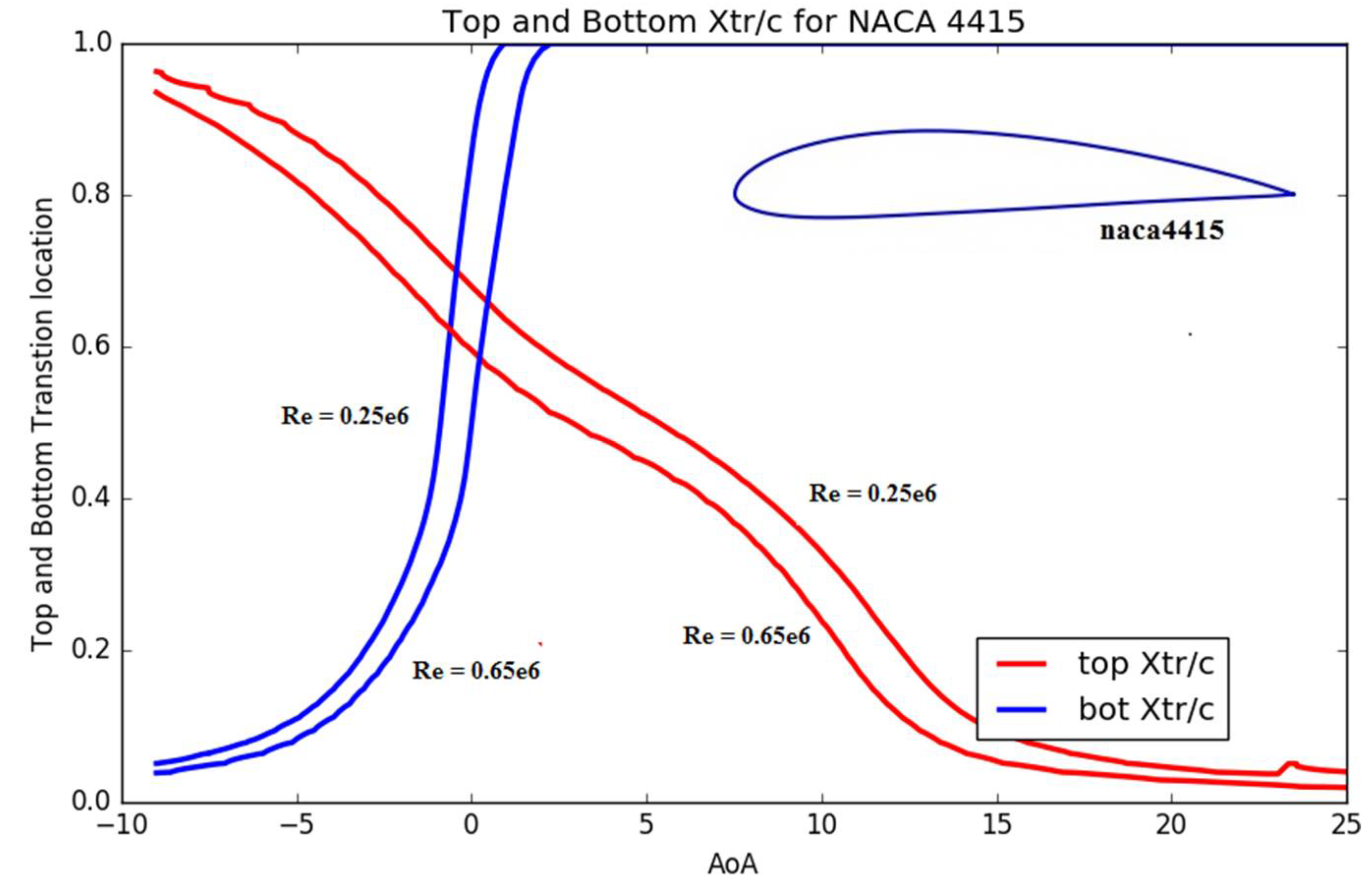
Transition location is crucial in understanding the onset of turbulence and relates to the skin-friction drag-and-stall phenomenon. At high AoA, the transition to turbulence occurs near the leading edge on the top surface as calculated by XFOIL. Figure 5 shows the transition location normalized by chord (Xtr/c) variation with different REYN for a range of AoA for NACA4415 airfoil. The top surface transition location decreases with the increase in REYN, and vice versa for the bottom surface transition location for a range of AoA, showing the dependence of the turbulence on the speed of the flow.
2.2. Low-Fidelity Design, Off-Design and Verification Using BEMT Tool
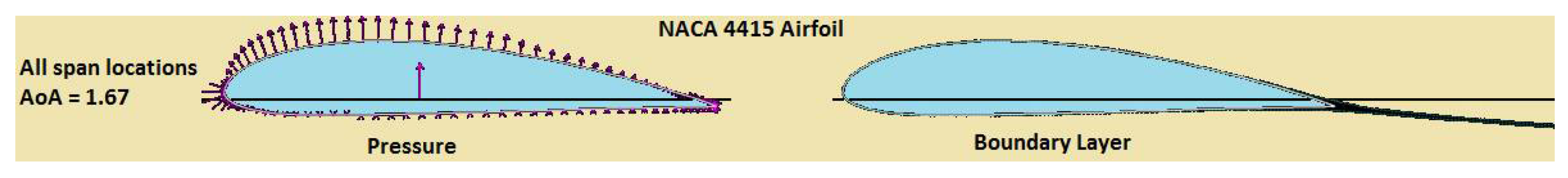
A sample propeller design for a light aircraft based on the work conducted by Adkins et al. [35,36] was chosen to replicate, and the specifications are shown in Table 1. The design is based on BEMT, and generated an optimum propeller using empirically minimized drag. NACA4415 airfoil is used for airfoil polar. The momentum loss is minimized by constant displacement velocity with constant AoA of 1.67° and the viscous loss by choosing a distribution such that minimum drag-to-lift ratio is achieved spanwise. A constant value of is chosen throughout the span. Using the specification and given chord distribution, it is reverse-engineered through py_BEM with airfoil polar from XFOIL runs. Fluid properties chosen are air at 20 °C with a density of 1.225 and kinematic viscosity of 15.68 × 10⁻⁶ . Table 1 lists the design specifications for the reverse-engineered representative blade using py_BEM.
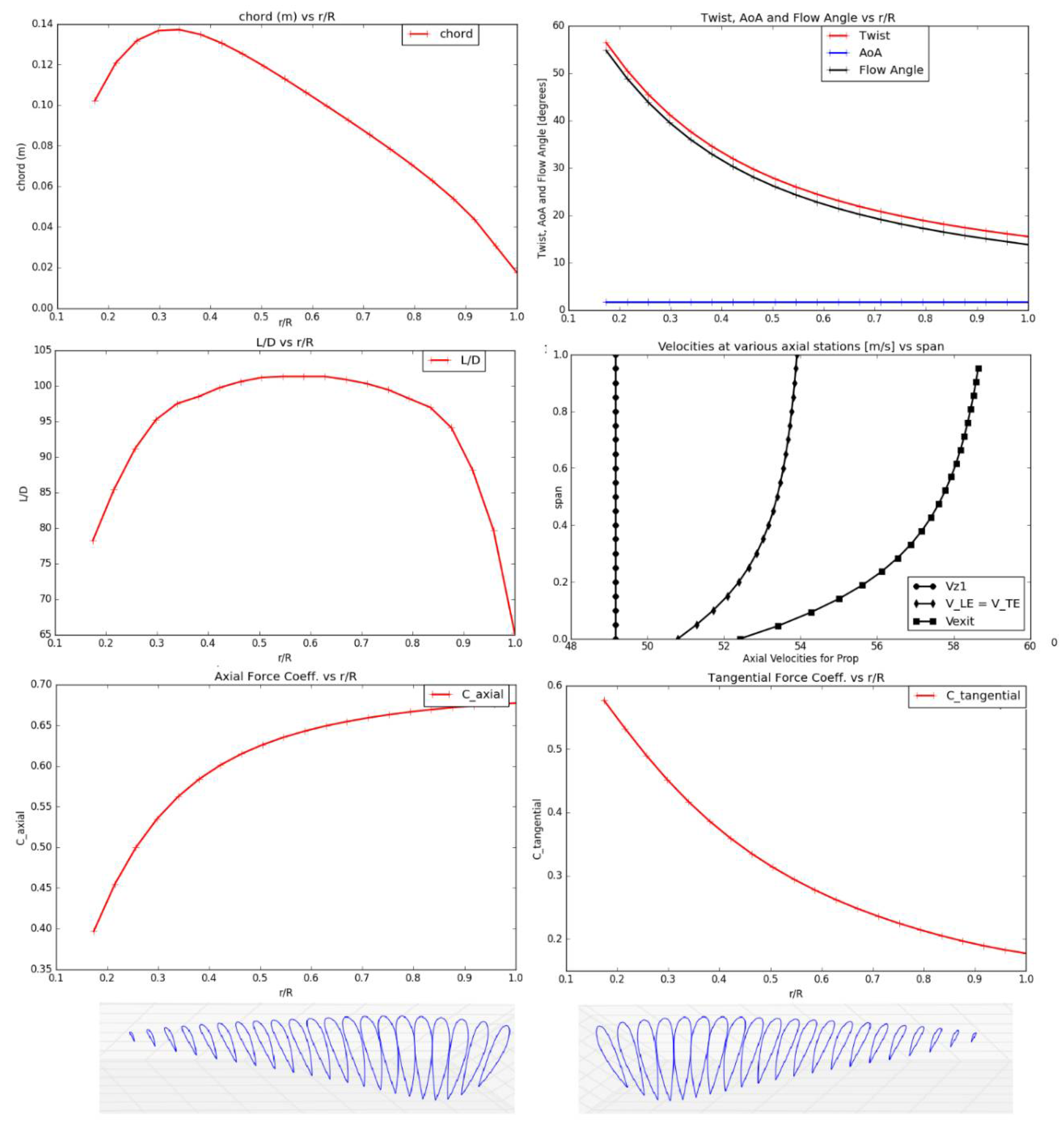
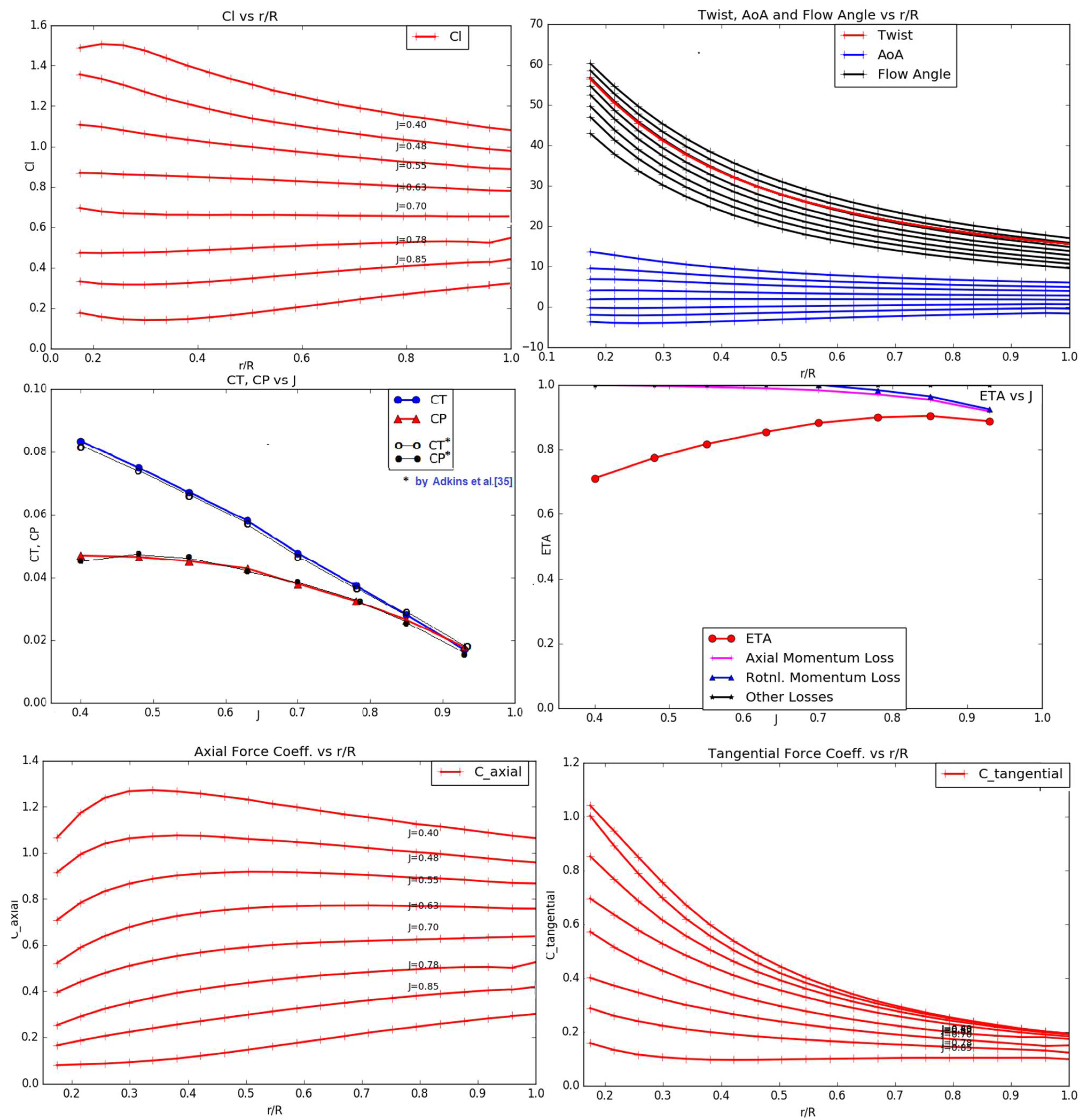
Figure 6 shows the NACA 4415 airfoil analyzed in Xfoil at AoA 1.67 degrees. Figure 7 shows the spanwise properties such as chord, twist, AoA, flow angles, lift-to-drag ratio, axial velocity spanwise and axial and tangential forces of the design generated. Reynolds number is varied spanwise. The above design point is used for an off-design analysis for various advance ratios by varying the flow speed at constant rotation. The chord and twist are kept constant at the design condition. The analysis result is also verified with the results obtained by Adkins et al. [35,36] and matches very closely as shown in one of the subfigures in Figure 8, which compares and with the advance ratio. It also shows spanwise aerodynamic properties for a range of speeds (advance ratio) at off-design points.
2.3. 3D Geometry and 3D Simulation Setup
Spanwise geometric properties obtained from py_BEM tool are used to create a 3D blade geometry for high-fidelity CFD using NACA4415 airfoil stacked at 30% chord with a flat tip [30]. Fluid flow simulation for an unducted rotor involves modeling the far field to capture the wakes far downstream, streamtube expansion or contraction and the effect of angular momentum change in the radial direction. Choosing the right fluid-domain size to capture these behaviors is crucial in improving the accuracy of the performance of the rotor. In addition to the standard mesh-dependency study, the domain-size dependency study is performed to define a required size for quantitative and qualitative analysis of the flow downstream of the rotor to conserve computational resources and improve accuracy.
The Spalart–Allmaras turbulence model, AGS and fully turbulent transition models are used in the 3D steady RANS solver by Numeca’s Fine/Turbo [41].
The general Navier–Stokes equations in Cartesian frame are given above, where Ω is the control volume and S is the control surface, is the set of conservative variables, and are the advective and diffusive part of the fluxes, contains the source terms, are the effects of external forces and is the work performed by the external forces [37]. The time derivatives are not calculated for steady solution.
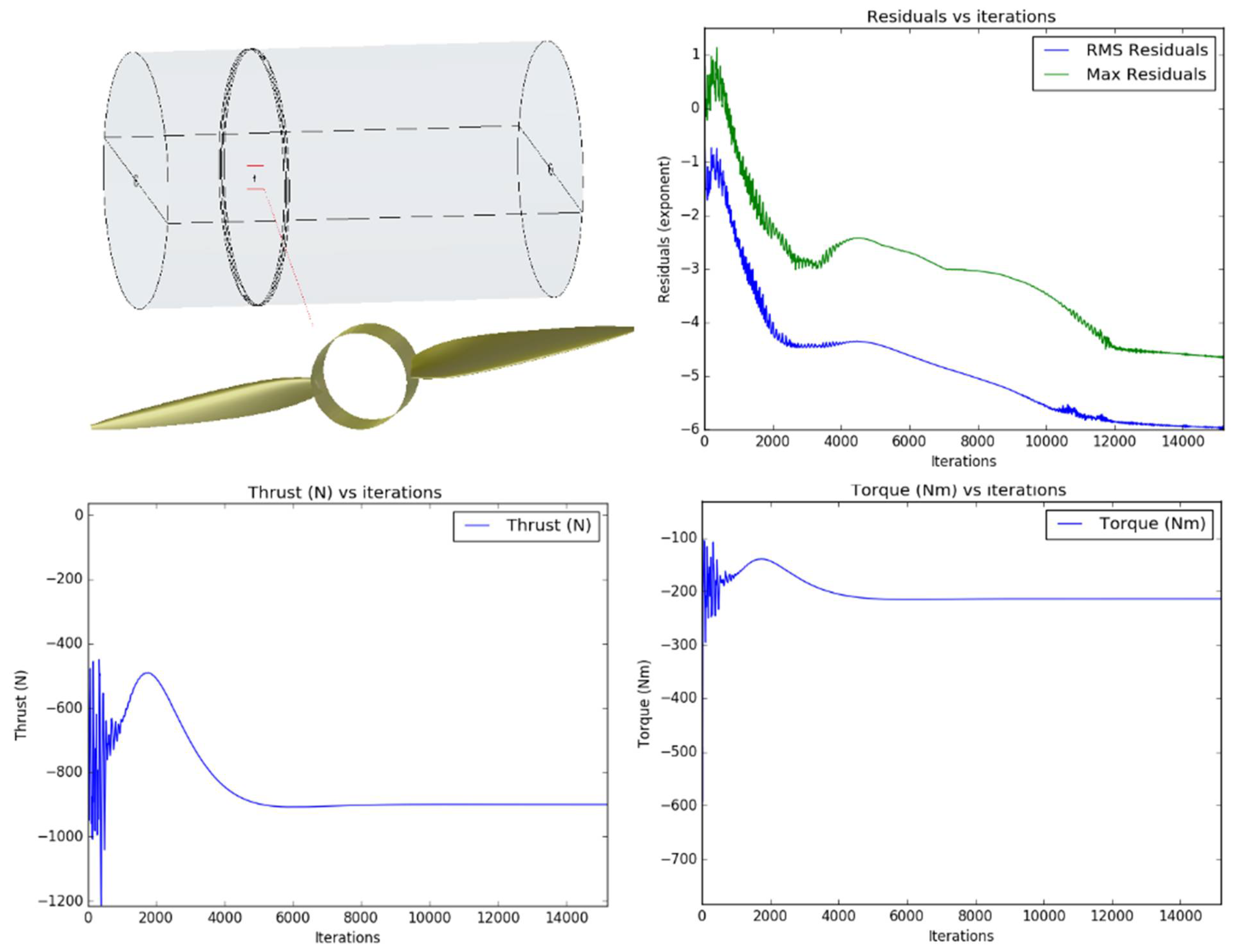
A cylindrical domain is created with upstream, far-field and downstream distances as a function of the blade radius, as shown in Figure 9 using Numeca’s Autogrid mesher. These distances are increased in a systematic manner starting from 5R-5R-10R (referred as 1X) to study the effect of domain on the flow convergence and behavior. In some cases, just the downstream distance is varied to examine the wake deficit and dissipation much further away from the rotor. More details of multigrid and mesh topology are present in Siddappaji’s work [37]. Thrust and torque values are monitored to obtain solution convergence, as shown in Figure 9.
The objective of the 3D steady RANS is to solve for the flow properties upstream, far-field, across the rotor and downstream in the prescribed cylindrical domain with a periodic mesh with repetition equal to the number of blades, which is 2 for this case. There is no inlet or outlet boundary condition to be defined, since this is an external flow analysis problem. Keeping all the solid patches as adiabatic, the external boundary conditions are set as atmospheric static pressure, static temperature and velocity normal to the Z axis as 49.17 m/s. Choosing the SA turbulence model, the default turbulent viscosity ratio is used. The Euler’s wall condition is applied to the nonrotating hub part, which is inviscid, and for the rotating parts, the Navier–Stokes wall condition is applied with constant rotation speed as specified. The initial conditions are identical to the external boundary conditions.
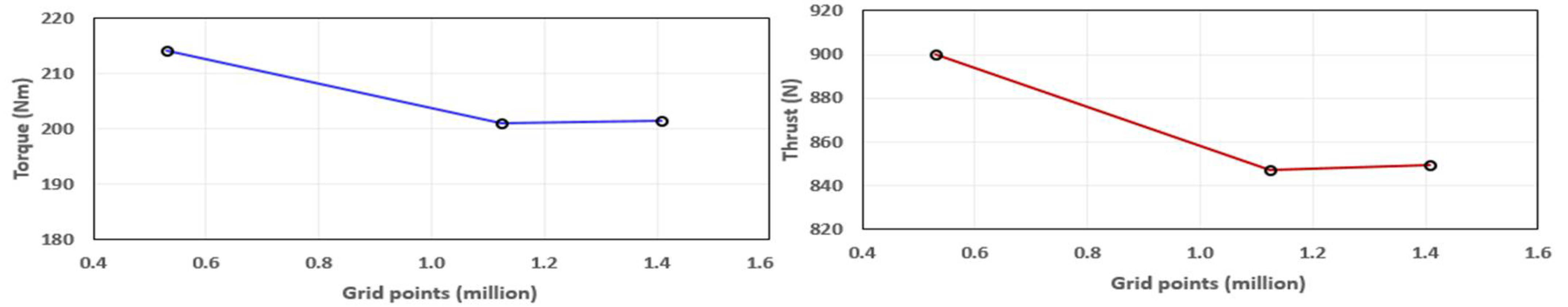
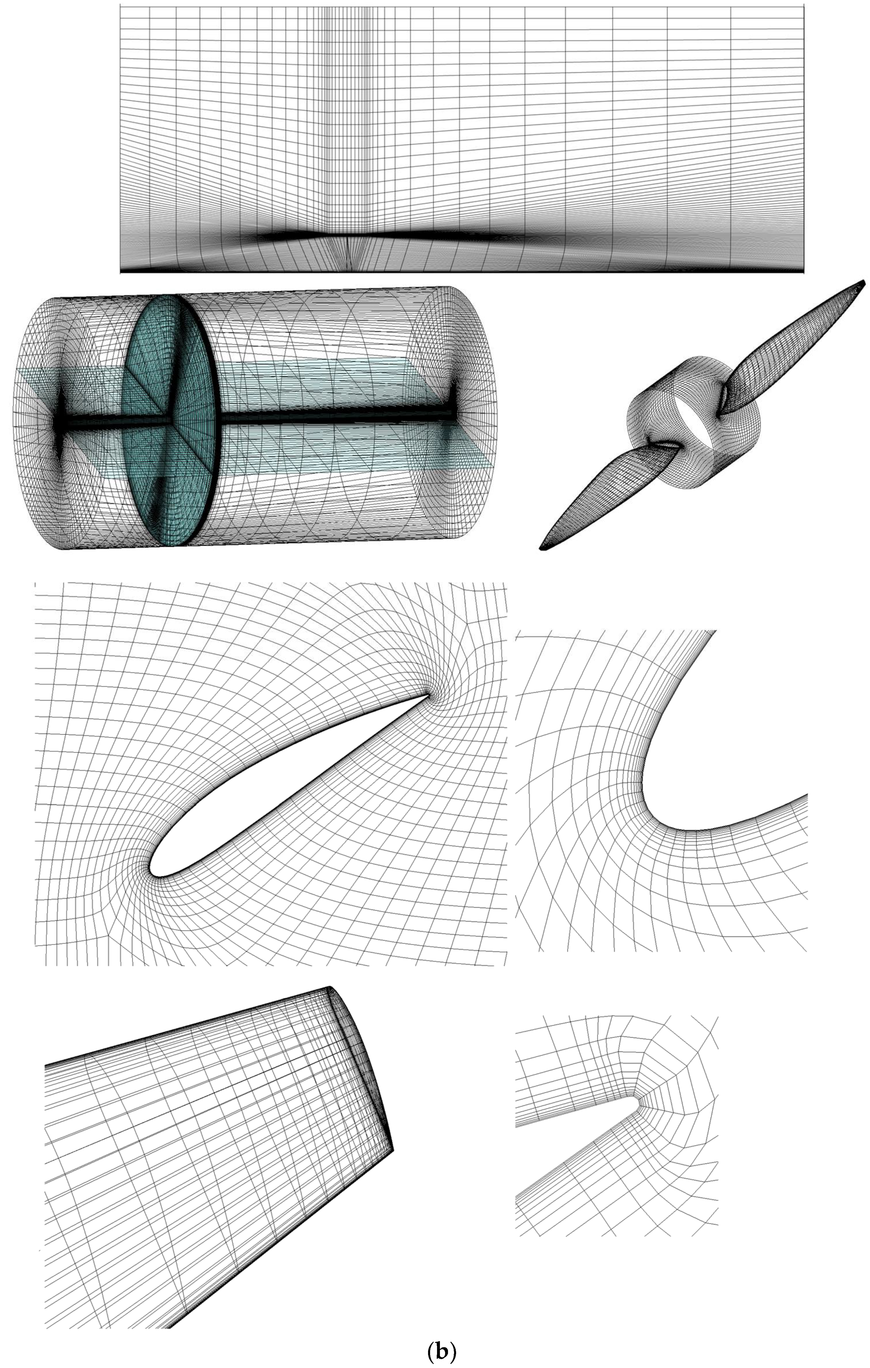
A grid-dependency study is performed with values of these blades between 1–8 indicating good quality of mesh for flow analysis to ensure the accuracy of the solution. Figure 10 shows three levels of grid density with thrust and torque values for various levels, demonstrating that after a certain number of grid points these values do not change significantly. Axisymmetric meshes for several domain sizes are compared in Figure 11a, keeping the region around the blade dense and similar across the domain sizes and sparse downstream. A typical mesh around the blade for domain 1X is shown in Figure 11b. 4X_AGS domain size is chosen for the grid-dependency study of the propeller design and for further flow analysis. Mass averaged absolute velocity magnitude for the corresponding domains in azimuthal (axisymmetric) views are also shown in Figure 11a, which demonstrates that a longer downstream domain is essential to capture the flow behavior since it takes longer than 5D to mix out to the upstream velocity.
Grid quality is an important measure of solution accuracy, and comprises aspect ratio, orthogonality, face skewness, stretch (expansion) ratio and Jacobian of the grid generated. The 3D grid depends on the curvature and aspect ratio of the geometry modeled. Poor quality grids hinder solution convergence and sometimes introduce solution instability. Standards for orthogonality-minimum (>20), stretch ratio-maximum (<2) and aspect ratio-maximum (<5000) have been established [34]. Figure 12 shows the periodic grid and metrics for the two-bladed propeller rotor and are within these limits.
3. Results
3.1. Comparison between Low and High Fidelity
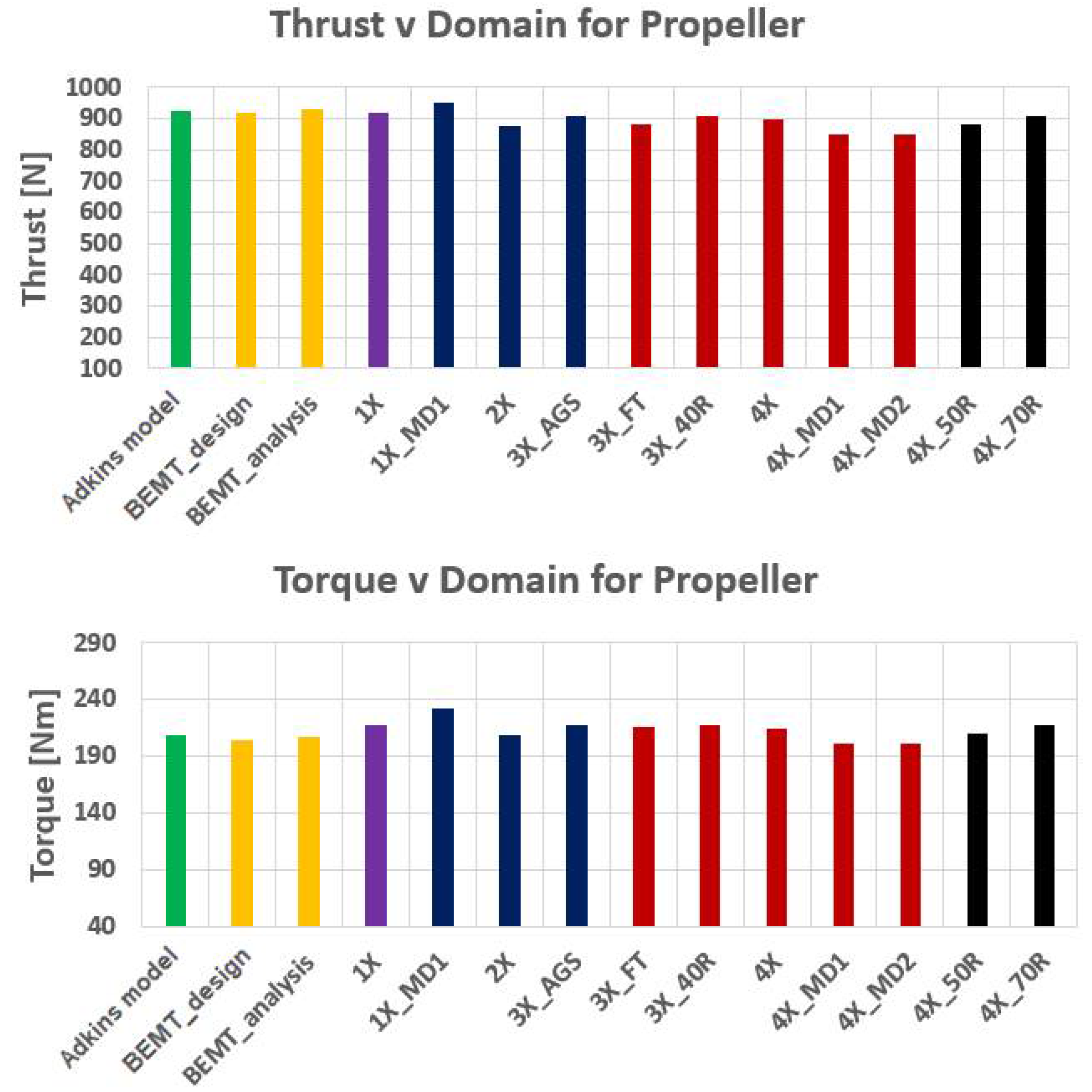
Device thrust, and torque values calculated from py_BEM are compared with results from 3D steady solution for several domains, and the difference lies within 5–7%. py_BEM treats the blade as a line of several radial stations, while a detailed 3D blade shape is analyzed in 3D RANS solution. Tabulated airfoil polar data is used in py_BEM to calculate forces on the blade, while 3D RANS solver obtains it by numerically solving the Navier–Stokes equations with turbulence and transition models incorporated [41]. Differences are observed due to 3D effects, root and tip vortices, flow separation, domain and mesh size, blade-surface mesh details, and the mesh quality.
Figure 13 lists the thrust and torque for various domain sizes compared with BEMT results and Table 2 provides grid details on blade and far field span layers, domain and mesh size. The design named ‘BEMT_design’ is obtained using py_BEM in design mode, defining the chord and calculating the flow and stagger angles, while the design named ‘BEMT_analysis’ is obtained by using the given AoA, chord and flow angles as stagger angles [35,36].
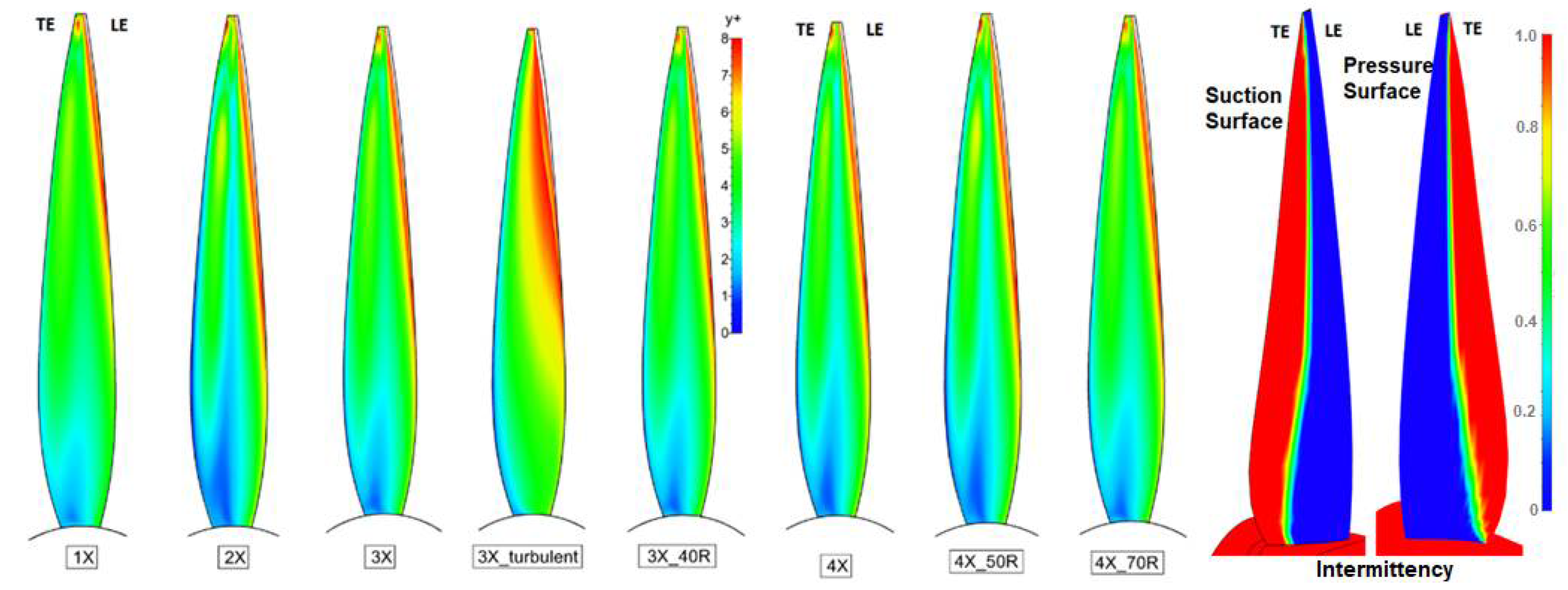
Figure 14 shows the contour plots on the suction surface for all the domain sizes analyzed, showing the variation between 1–8 due to different mesh count. It also shows the intermittency on the suction and pressure side obtained from the 3D RANS solution with the AGS transition model. The chordwise transition from laminar to turbulent flow in the boundary layer throughout the blade span is shown here. Laminar flow is at zero and fully turbulent flow is at unity. Transition starts when the intermittency deviates from zero and is highly dependent on the angle of attack, airfoil shape and Reynolds number.
Figure 15 shows spanwise distribution of thrust and torque compared between py_BEM and 5R-5R-10R domain 3D RANS solution, referred as 1X. It also shows spanwise thrust distribution compared with several domain-sized 3D RANS solutions and the flow angles for the blade. The hub vortex in the 3D solution causes the tiny bulge in thrust curve for 0–10% span while py_BEM does not calculate hub losses. In addition, near 85% span, tip losses are more pronounced in the 3D solution due to the 3D effect and grid resolution. As the downstream distance is increased, spanwise distribution moves close to BEMT results, as seen in 4X_70R_AGS case. Flow angles calculated in 3D RANS solution follow the same trend as calculated by py_BEM but is offset by a small degree because of the location where these values were calculated in a mass-averaged azimuthal plane.
3.2. Momentum Transport and Wake Analysis
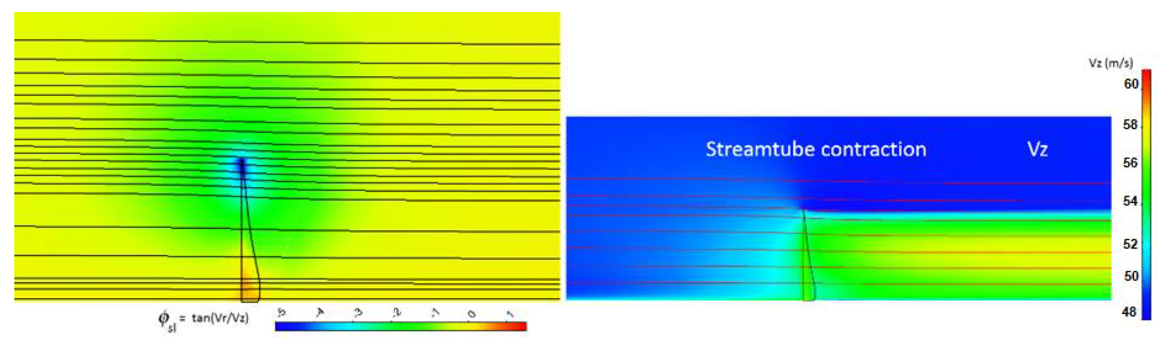
BEMT is partly based on axial momentum theory, where the axial momentum and velocity can be tracked downstream of the rotor to analyze energy exchange. A propeller creates thrust by increasing the velocity in the immediate downstream, and due to the continuity principle, the exit area is reduced from streamtube contraction. Figure 16 shows the streamtube contraction near the solo propeller rotor. The slope of the streamline is negative in the top 60% span where the most thrust comes from velocity increase, while near the hub, the slope is slightly positive. The benefit of 3D CFD is that several properties can be tracked in all three directions for a steady case to understand the transport phenomena.
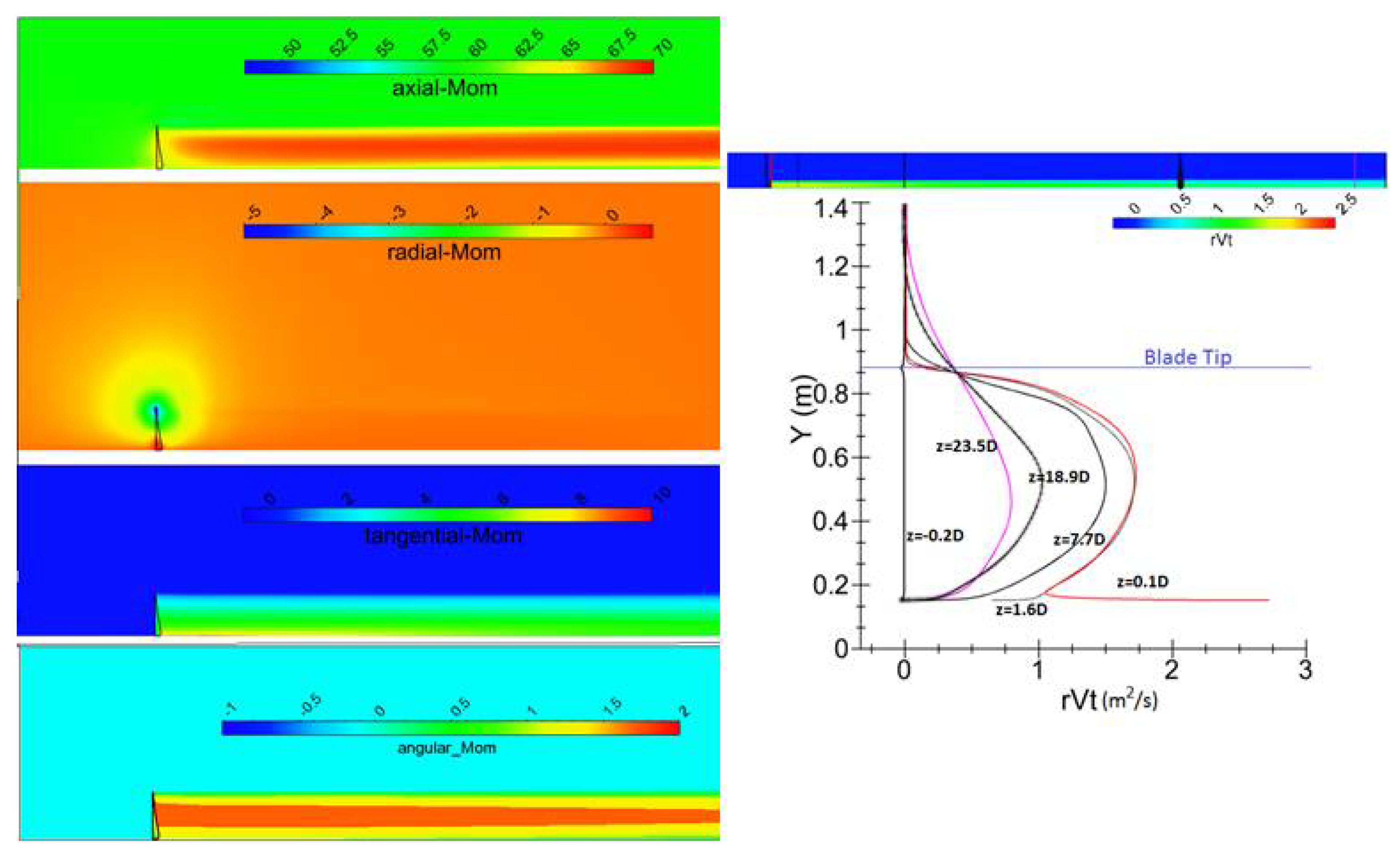
An azimuthal view of mass-averaged axial, radial, tangential and angular momentum is plotted for 3X domain (15R-15R-30R) and shown up to 8D downstream of the rotor in Figure 17. The momentum ranges are not kept the same in order to pinpoint which momentum has a major contribution in entropy rise. It is very clear that the axial momentum has a larger contribution towards the entropy rise among all other momentum, as it creates stronger wakes downstream of the rotor. Radial momentum transport occurs even above rotor height, as shown in the figure, which primarily causes streamtube contraction.
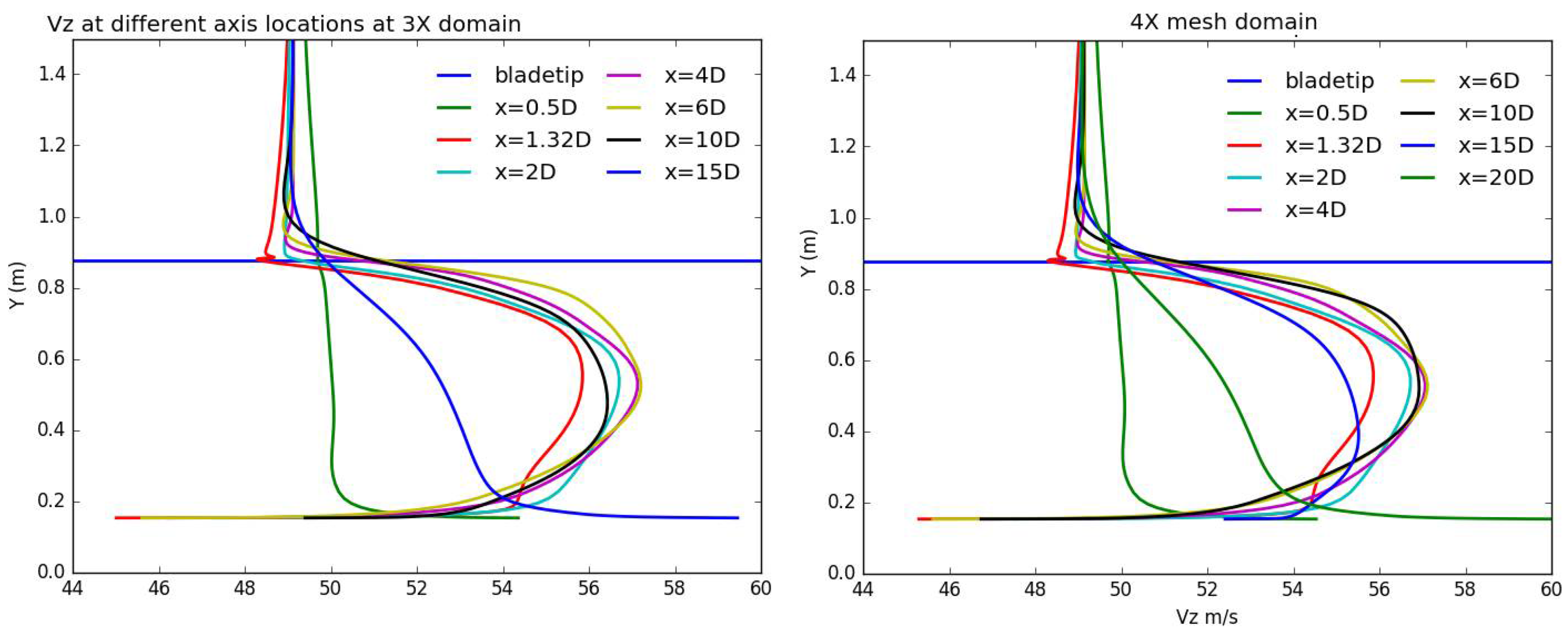
A closer look at the wake decay in domains 3X and 4X is shown in Figure 18. The largest wake profile is at 6D, after which the wakes start decaying to reach the inlet velocity, indicating mixing with free stream between 6–10D downstream. The wakes also show that at 6D and beyond, there is radial growth, indicating vortex expansion. The wakes are reduced mostly by viscous dissipation in solo rotors, increasing the entropy. It demonstrates the fact that performance improvement can be achieved by reducing the wakes using another rotor instead of allowing energy to dissipate downstream.
One of the assumptions in this work is constant velocity at the inlet and no distortion, which if present, affects the wake decay. An energy-exchange designer must keep this in mind and take advantage of it while designing rotors through boundary-layer ingestion or exit swirl. Swirl exiting the propeller is tracked using angular momentum as shown in Figure 17 for the 4X_70R domain at 0.1D, 1.5D, 7.7D, 18.9D, and 23.5D. It is maximum at 0.1D, which is very close to the trailing edge, and then starts decaying while varying between 0–2 .
3.3. Vorticity Dynamics and Entropy Increase
The curl of momentum equation in the set of Navier–Stokes equations for an incompressible Newtonian fluid gives the vorticity transport equation, as shown in Equation (8) where is the vorticity vector, is the velocity vector and is the kinematic viscosity, which is assumed to be uniform and constant [20].
The above equation shows that vorticity changes either because of vortex stretching (first term on right-hand side) or due to diffusion into the flow because of the viscosity effect caused by friction. This vorticity diffuses in the boundary layer and is convected downstream, which eventually becomes a wake leading to a drag and rise in entropy. Vorticity dynamics is another method of viscous flow analysis that tracks radial vorticity and boundary vorticity flux on the blade boundary layer.
Vorticity created in the blade boundary layer, trailing edge and at the tip are contributing factors to turbulence noise and performance loss. Rotor rotation causes hub and tip vortices to propagate downstream in a helical path until it mixes out, increasing the entropy all along. The Y component of vorticity in the ZY plane (Z axis as the axial direction) downstream of the solo propeller rotor is shown for the 3X-40R domain in Figure 19.
It also shows spanwise plots of the vorticity_Y and the entropy created at several axial locations: −0.2D (front of rotor), 1.6D (right behind the rotor), 7.7D (near mixing) and 18.9D (very far downstream). The vorticity line plots show hub vortex development up to 25% span as we move away from the rotor (red line at z = 0.1D) and vortex stretching increases it to 50% span near mixing at around 8D and starts dying down, as seen in the far-downstream location. It is important to notice that the vorticity is negative from the hub to midspan and is positive above the midspan. The hub vortex has circulation with opposite sign to the tip vortex and is rotating in the opposite direction to that of the tip vortex. BEMT does not account for the radial flow from hub to tip because of its assumptions. After z = 7.7D, which is near the mixing location with the free stream from above, vorticity_Y reaches beyond the tip due to vortex stretching shown by black line. Spanwise plots of entropy at the above-specified axial locations in the figure show that there is a jump near the mixing location and increases beyond for this domain. After the mixing location, the spanwise entropy lines extend beyond the tip location, demonstrating the rise due to mixing of wake and free stream flow.
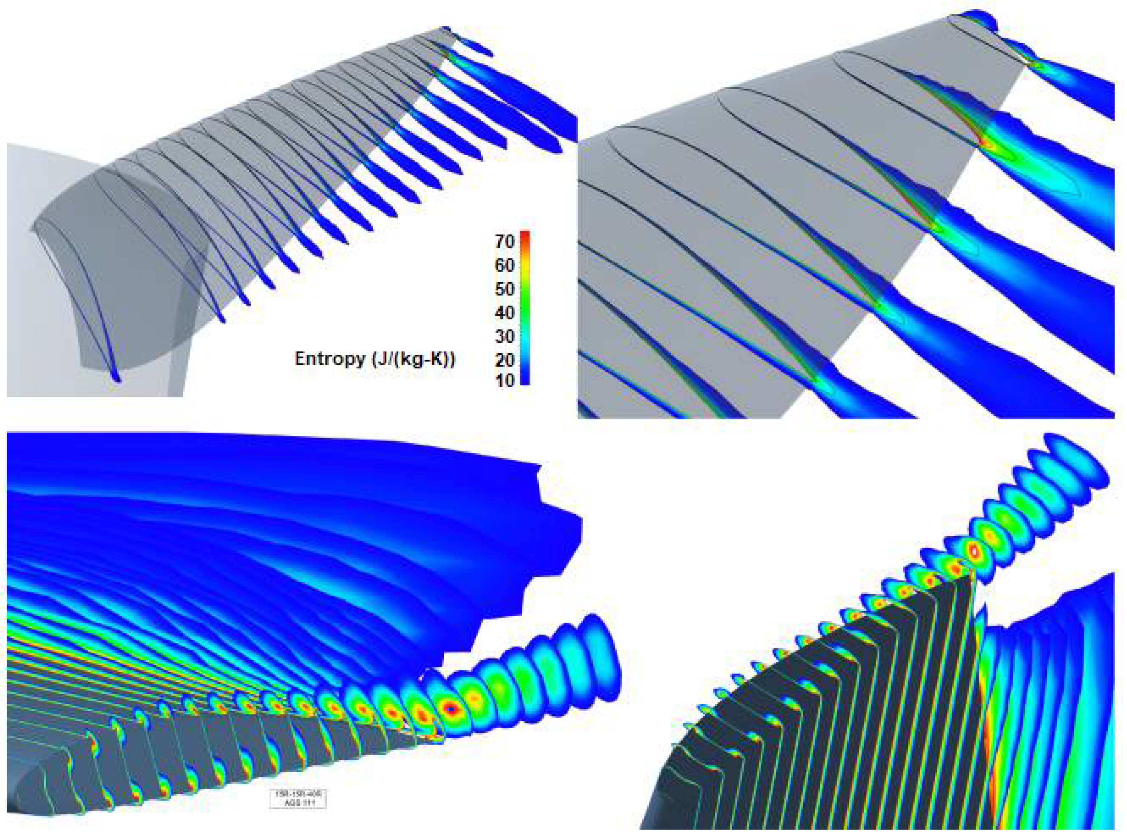
In Figure 20, entropy contours at several planes through the blade and downstream show the tip leakage and mixing from pressure to suction side, creating tip vortices for the 3X-40R domain steady solution. It also shows the entropy at several radial planes with mixing at the trailing edge, causing the entropy to rise and propagate downstream. The blade design has a flat-tip geometry, which affects the tip leakage substantially and can be improved by making a smoother tip, winglet tip or a split tip [37]. As the rotor spins, these tip and hub vortices move in a helical path. The benefit of using entropy as a measure of loss is that it is independent of the reference frame, so there are no relative terms to keep track for a rotor, rendering it the most accurate thermodynamic measure of performance.
Boundary vorticity flux (BVF) measures the amount of vorticity diffused in or out of the surface per unit area and unit time. It also relates to the amount of circulation, which leads to lift, boundary layer development and separation onset. BVF is defined in an equation as using kinematic viscosity and vorticity and is split into contributions of the wall acceleration , on-wall tangent pressure gradient, and a 3D viscous correction, of which for a large Reynolds number, only dominates [37]. BVF indicates the onset of flow separation or its existence on the blade shape by calculating the flux from the blade surface diffused into the boundary layer before being propagated downstream.
Radial vorticity on the blade wall shows the circulation distribution, transition from laminar to turbulent flow and onset of flow separation. Along with skin-friction vectors, more crucial information about the flow dynamics can be analyzed. The axial component of BVF due to the on-wall tangent pressure gradient is another key parameter to observe in order to understand vorticity dynamics. There are three criteria for boundary-layer separation established using skin friction and vorticity vectors along with BVF on blade wall, and these are as below:
- Separation zone warning: skin-friction vector lines () converge, vorticity vector lines () have large positive curvature and BVF has a peak.
- Separation line criteria: curvature of vorticity lines reaches a maximum.
- Separation watch: Tangent BVF lines turn towards the direction of skin-friction vector lines or tangent pressure-gradient vector lines are normal to the separation line.
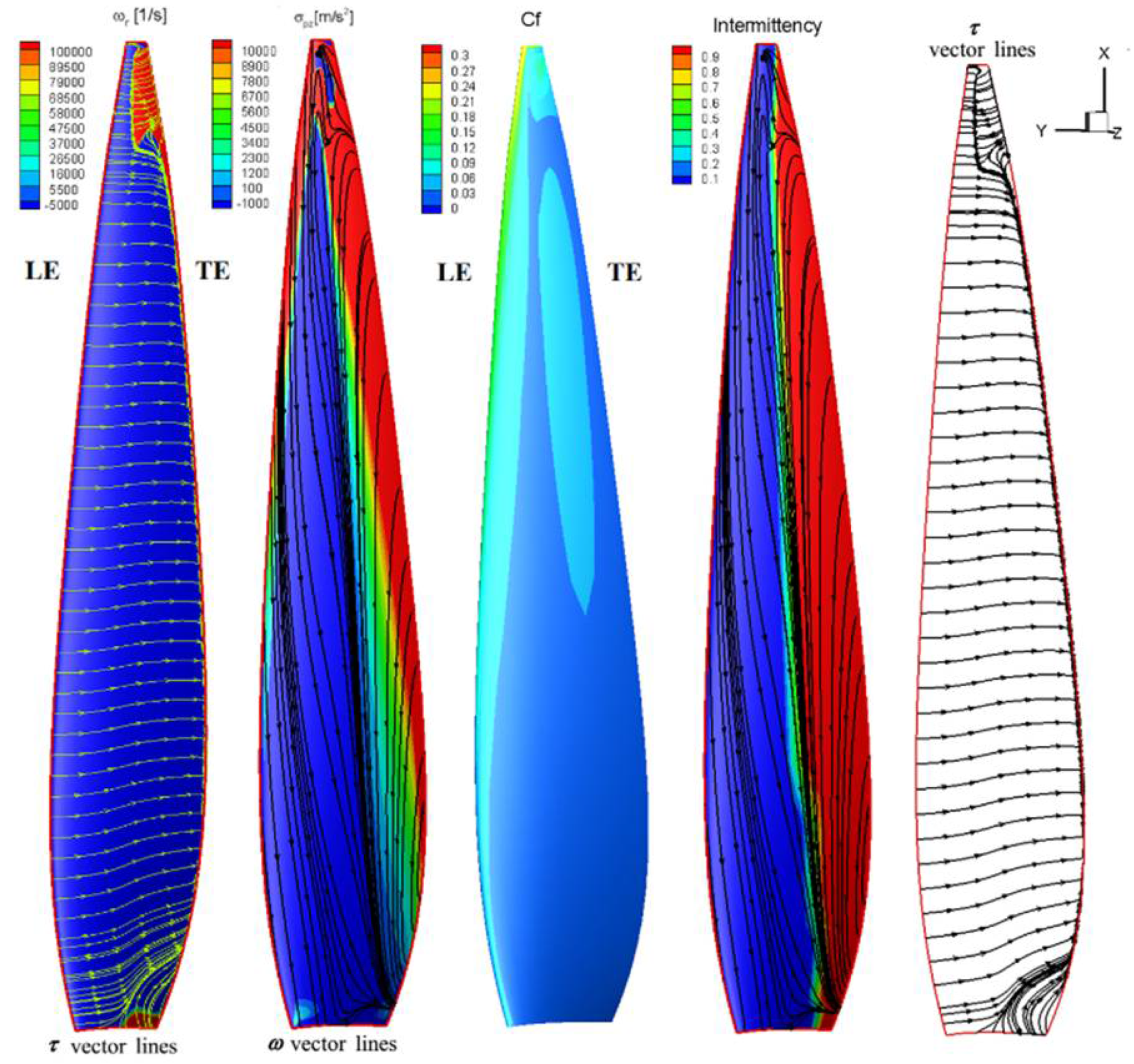
Figure 21 shows radial vorticity, BVF, skin friction and vorticity vector lines, skin friction, , intermittency calculated using the AGS transition model and entropy gradients plotted on the suction side of the solo propeller blade for the 3X-40R domain 3D steady solution. It shows a comprehensive correlation between these properties, giving a summary of the flow behavior in the boundary layer prior to downstream propagation. These relationships are explained in detail by addressing several groups of those contour plots further. On-wall radial vorticity with skin friction vector lines, BVF due to tangent pressure gradient with vorticity vector lines and skin friction contours for suction side of the solo propeller with 3X-40R domain steady solution using AGS transition model and Z being the axial direction are shown in Figure 21.
The first plot shows that most of the flow on the no-slip wall is clean flow, except the top 15% and near the hub. There is an onset of flow separation in the top 15%, shown by the skin-friction vector lines converging, and are lined up well at the boundary of very high values of radial vorticity. The sign change in radial vorticity also depicts the flow separation. The second plot shows the vorticity vector lines on the BVF contour due to pressure gradient in axial direction with curvature of vorticity vector lines reaching maximum on the separation line satisfying one of the criteria. A higher positive peak is not favorable for the design as it reduces the torque on the rotor and can be seen in the second plot, which lines up well with the vorticity vector lines with higher curvature. The BVF and radial vorticity distribution on the blade affects the skin friction, as shown in the third plot in the same figure. Clearly, there is a high skin-friction zone near the top 15% due to the turbulent boundary layer caused by positive peak.
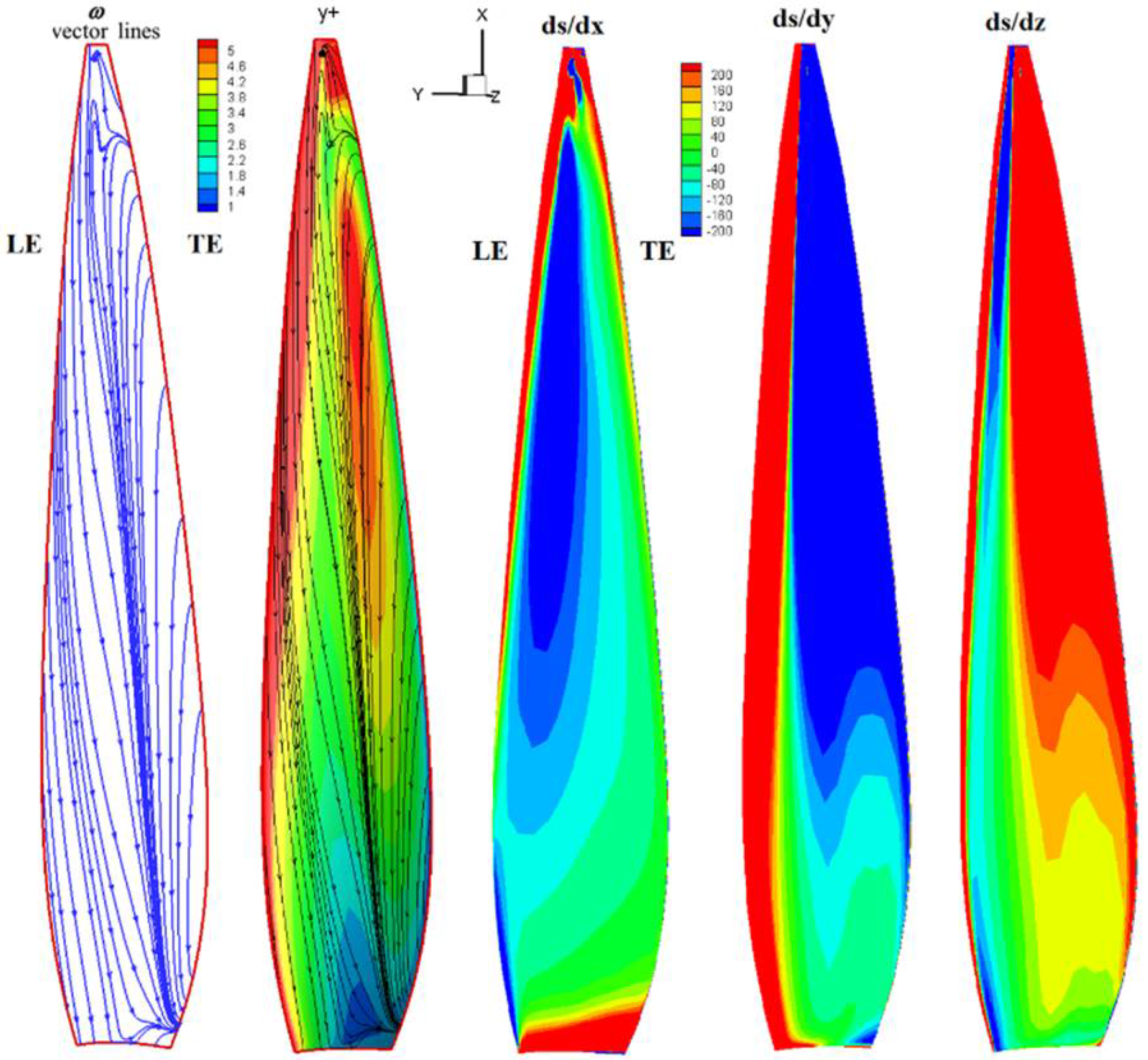
Figure 21 shows the intermittency calculated from the AGS transition model depicting the onset of turbulent flow as the value moves closer to 1 with vorticity vector lines overlayed on it. These vector lines converge at the point or zone of transition due to a higher shown in the previous figure. The figure also shows skin friction and vorticity vector lines on the suction surface, which are normal to each other, to obtain a clear picture of the on-wall signature of the turbulent flow and flow separation. The vorticity and BVF distribution on the no-slip wall of the blade suction surface also dictates the entropy created and its change in all three directions, as shown in Figure 21. A lower gradient is desired, but due to the turbulent boundary layer, higher BVF peak and larger skin friction, the gradients are high after 50% chord in the X and Z directions. A closer look at the top 15% with entropy gradients, skin friction and vorticity vector lines reveal interesting turbulent flow structures shown here for the first time. The skin-friction vector lines are normal to the vorticity vector lines and converge at the onset zone of flow separation, which is also the transition zone for turbulent flow, causing the entropy gradient to increase. The turbulent boundary layer increases the surface vorticity, causing greater skin friction. The vorticity vector lines have larger curvature in the turbulent boundary layer, which is seen after a 30% chord in the figure. BVF analysis tells us that the top 15% span creates the tip losses, and is examined closely through skin friction, vorticity and entropy. A similar effect is seen near the hub depicting hub losses.
3.4. Kinetic Energy Dissipation as Entropy Rise
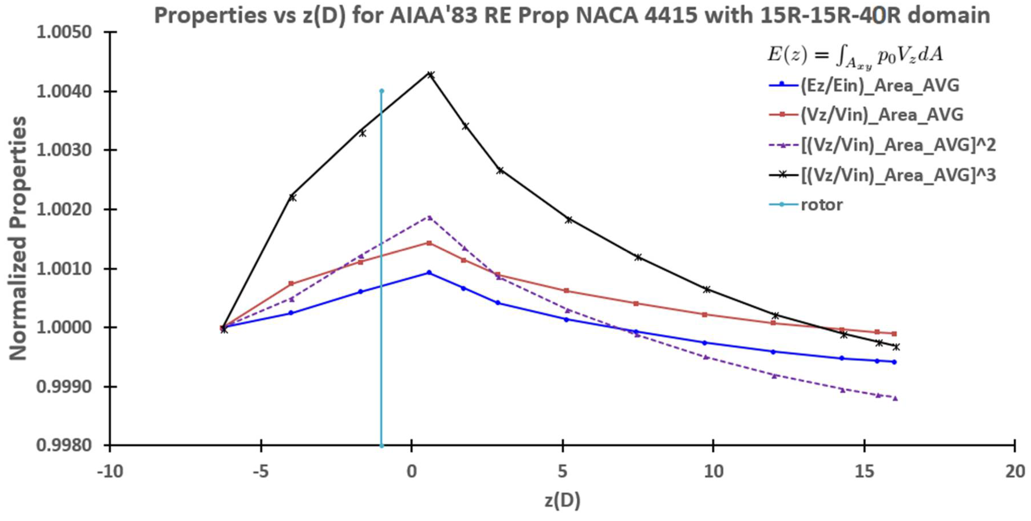
The propeller rotor transfers kinetic energy (KE) to the incoming flow, and a part of it is converted to thrust and the remaining dissipates, which also increases entropy. Similar to the momentum, the axial KE makes a major contribution to the entropy rise. Entropy is created due to viscous dissipation and heat transfer, but in case of incompressible fluid, the heat transfer part is neglected for unducted rotors, which is small compared to the dissipation term. KE is dissipated into the flow downstream of the rotor, and when the mixing occurs between the wake and the free stream, entropy rises significantly. The decay of axial KE downstream is a direct result of the dissipation, turbulence and the amount of vorticity in the wakes. The area-averaged and normalized velocity, KE and power at several axial locations downstream for 3X_40R domain are shown in Figure 22. The increase in energy is because of the transfer by the rotor, and it slowly decays as we go further away from the rotor.
Exergy, ξ, is not conserved in a thermofluid dynamic process and is destroyed due to irreversible processes within a system, and its quantification improves performance analysis. An exergy balance is appropriate for a control volume to assess the process more accurately. Exergy is removed from the system when energy is provided to the system and vice versa. The change in total exergy for a closed system is caused by the transfer of energy by work and heat between the system and surroundings [42]. Irreversibility, , quantifies the exergy destroyed in a control volume and is plotted for 20R-20R-70R domain case.
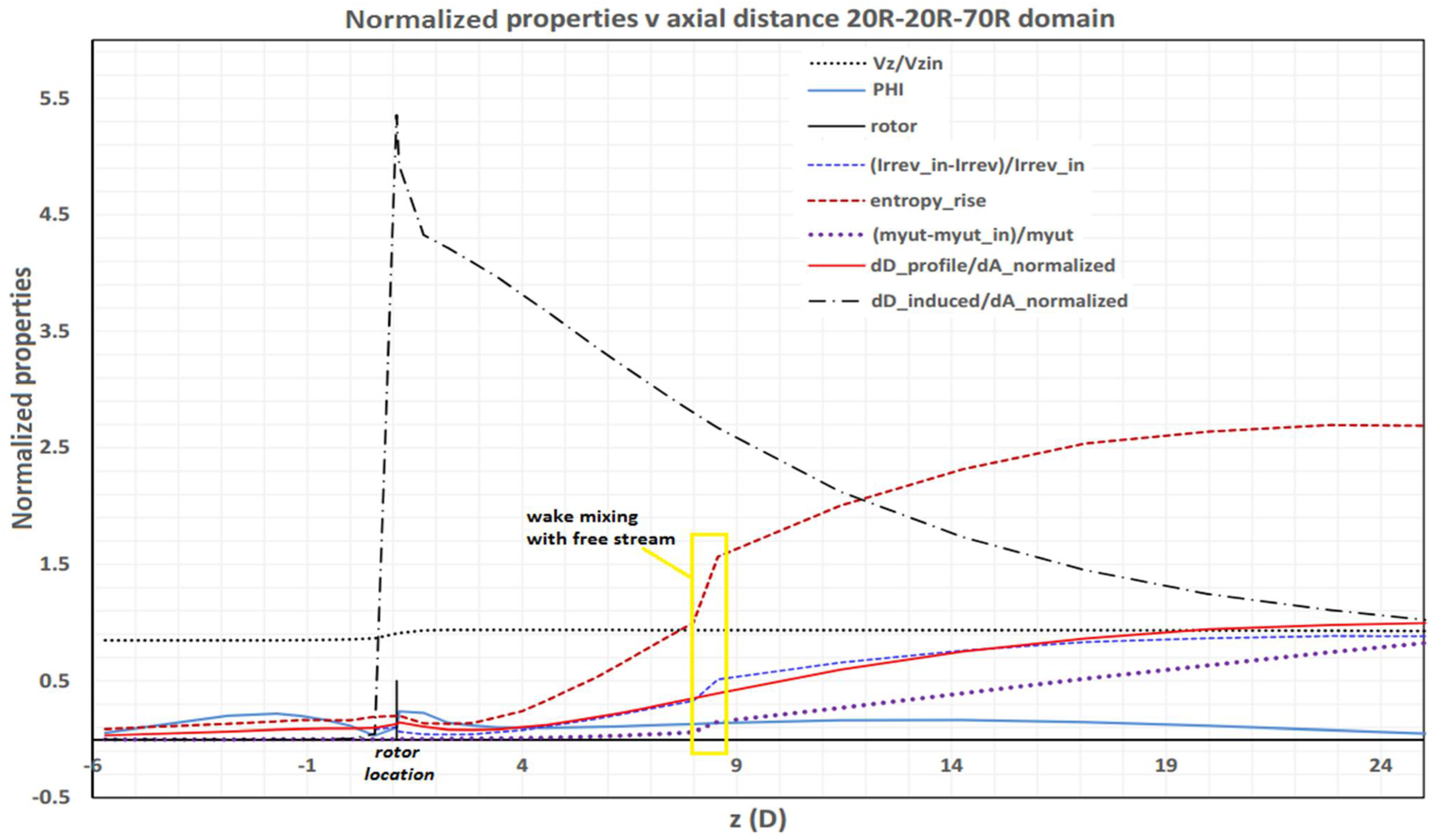
Dissipation function, normalized axial velocity, change in irreversibility, entropy rise, change in turbulent viscosity, profile and induced drag normalized by the area are tracked at several axial locations for the 4X-70R, domain as shown in Figure 23 for an exhaustive comparison and to see the behavior far downstream with the rotor location marked. These properties are mass-averaged line integrals up to radius = 1 m (>rotor radius) in the axisymmetric plane and are normalized to obtain a comprehensive understanding. Mixing occurs at around 8D downstream of the rotor when the tip vortices start mixing with the freestream flow, as seen in the figure where entropy, turbulent viscosity and irreversibility have a jump in values.
It also shows the normalized irreversibility increase downstream of the rotor at various axial locations in the blue dashed line, caused due to entropy production from the dissipation of kinetic energy, mixing of the wake with the free stream and due to the turbulent viscosity. This is exergy destroyed in the system. py_BEM calculates exergetic efficiency to assess the exergy budget of the propeller rotor.
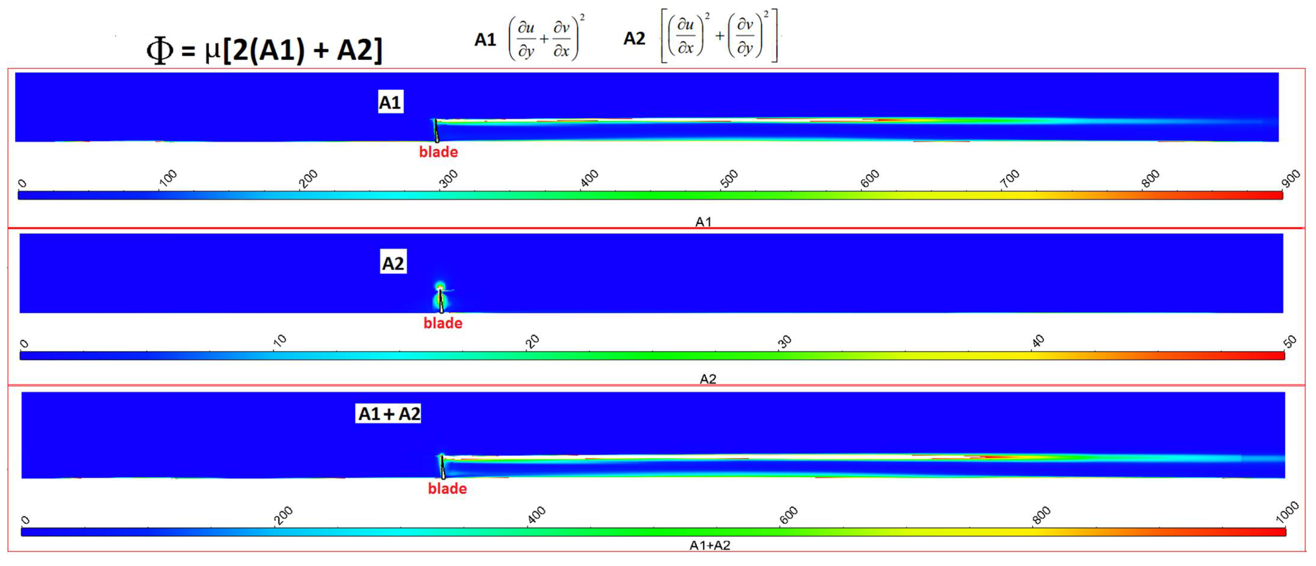
The mass-averaged dissipation function is split and plotted in Figure 24 to understand the contribution of velocity gradients and shear stress in axisymmetric plane. The shear-stress term A1 is wider-spread downstream than the velocity-gradient term A2, demonstrating why shear stress is vital in mixing.
3.5. Drag as a Form of Entropy
Total drag comprises of profile and induced drag for incompressible flow. Skin-friction drag is part of the profile drag. A Trefftz-plane analysis of these two quantities at several locations downstream is useful in understanding their propagation. Drag is another form of entropy. The Trefftz-plane integral equation can be derived from the momentum equation of Navier–Stokes set of equations assuming steady flow and neglecting body forces. Considering as cross-section areas of interest at an inlet and a plane downstream of the rotor, we have the equation for drag as below, and including the enthalpy-change equation, it can be split into profile and induced drag [24].
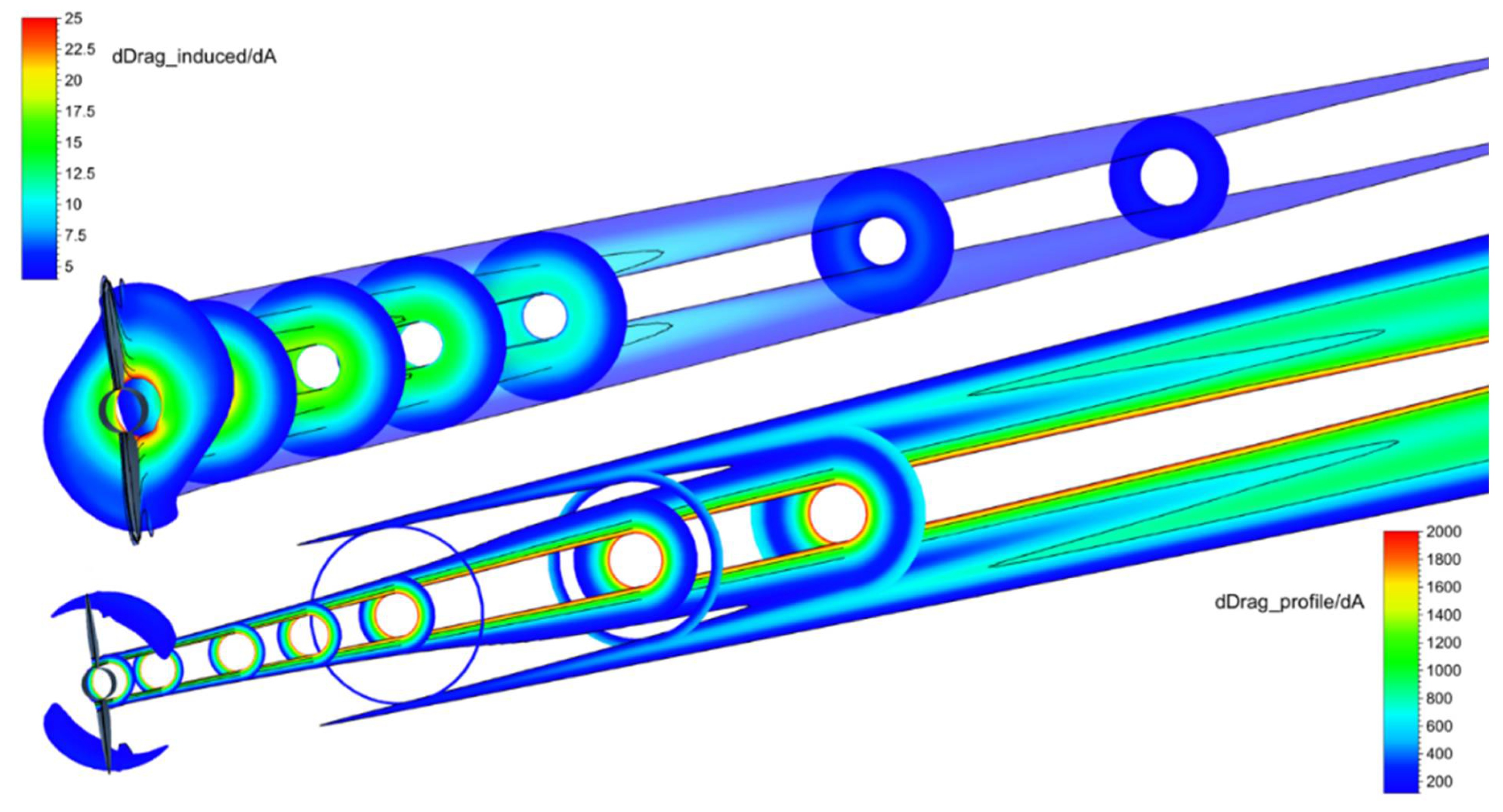
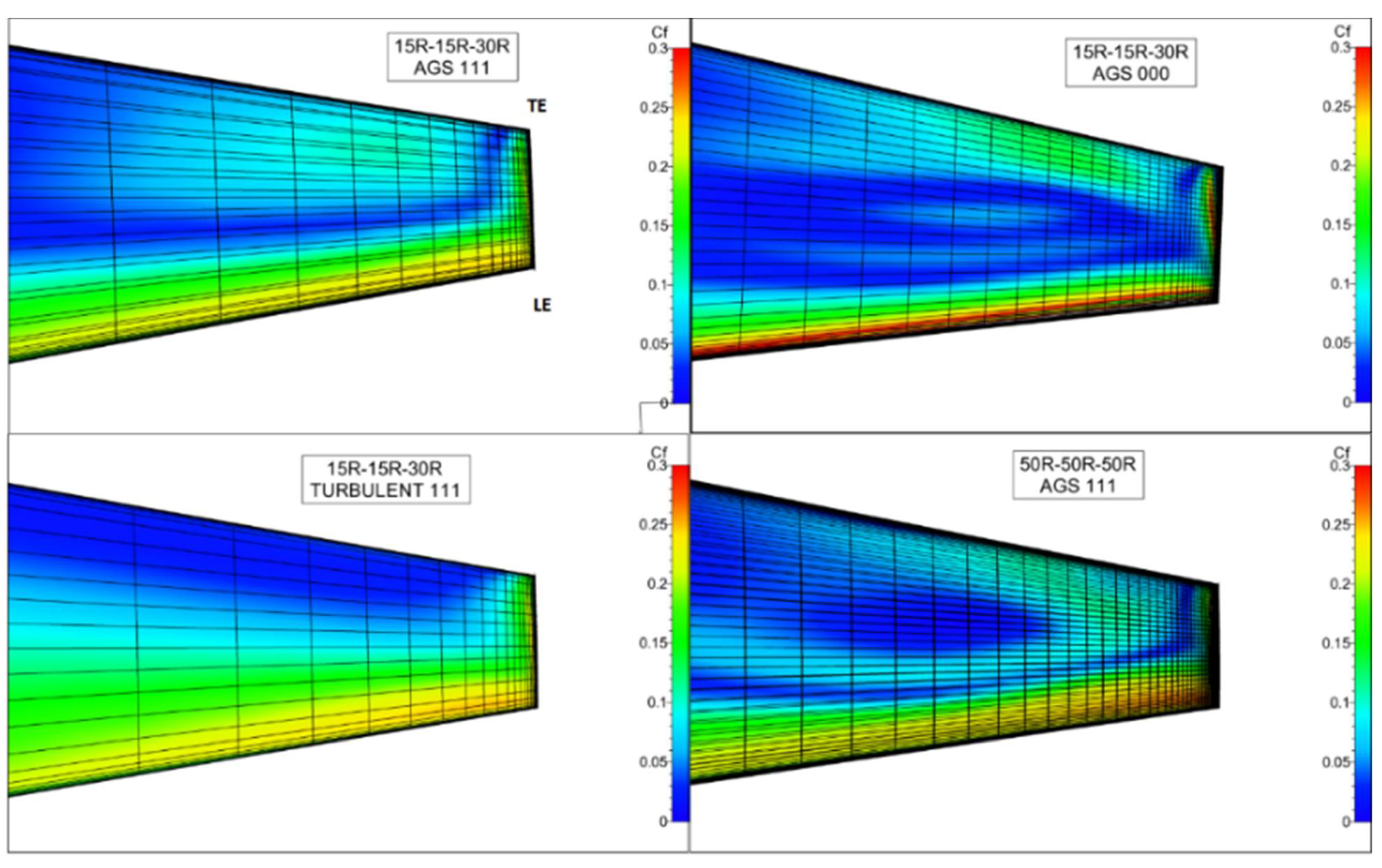
Figure 25 shows and at several axial locations downstream with an area of 1 m radius (>rotor radius), and is normalized with an inlet value. Figure 23 shows the contour plots of these quantities on an axial symmetry plane and cross planes at several locations downstream of the rotor. The profile drag starts increasing downstream as the entropy rise occurs. The induced drag is very high near the rotor due to the amount of lift generated, and slowly decays as we move away from the rotor, showing that the vortices shed in the wake are mixed out downstream. Skin-friction drag on the blade surface calculated numerically depends on the spanwise and chordwise mesh density and the transition model used in a turbulence model, as shown in Figure 26 and Figure 27. A higher mesh density is seen for 000 as compared to 111 in FINE/Turbo meshing nomenclature [41]. A fully turbulent model option is also applied other than the AGS transition model, with the Spalart–Allmaras turbulence model for the steady solution, and the skin friction is captured entirely differently, as seen in the figure indicating the dependence of modeling choice on the results obtained.
4. Conclusions
A solo propeller is designed using py_BEM at a low-fidelity level, and a 3D blade shape is created using T-Blade3 for higher-fidelity analysis. Several physics-based improvements are incorporated in py_BEM to address the local Reynolds number effect, boundary-layer rotation and airfoil polar at large AoAs, among others. Momentum, vorticity and kinetic energy transport mechanisms are described in detail to provide a comprehensive multifidelity flow-physics analysis. Wake analysis explains the streamtube contraction and mixing with the free stream. Domain and mesh-dependency studies are performed to understand the flow behavior far downstream in 3D steady CFD solutions. Vorticity dynamics is explained in detail, showing the importance of vorticity flux generated in the blade viscous boundary layer, and how it diffuses and convects downstream to create wakes. Several thermodynamic and fluid dynamic properties are tracked downstream of the rotor, and the intricacies of their relationship are explained to quantify the entropy rise. Flow mixing at the trailing edge and tip leakage causes additional loss and creates wakes. The tip and hub vortices are propagated further downstream in a helical path and cause entropy to rise. Kinetic energy dissipation transports the entropy further down into the wakes until mixing occurs with the free stream, and velocity far downstream reaches close to the free-stream velocity. All the components of drag are quantified to prove that drag minimization is a form of entropy minimization. Although py_BEM is a low-fidelity tool with certain limitations, including no radial flow, no 3D flow effects and constant velocity at the inlet, it is robust and accurate within realistic limits to provide a valuable performance measure during the early design stages, and combined with high-fidelity tools, provides a faster way to explore designs for trade-offs and enables multifidelity analysis. Future work will be to include wake-expansion models, introduce a radial flow effect, add a vortex model and improve loss models based on entropy.
Author Contributions
Conceptualization, K.S. and M.T.; methodology, K.S. and M.T.; software, K.S.; formal analysis, K.S.; resources, M.T.; data curation, K.S.; writing—original draft preparation, K.S.; visualization, K.S.; supervision, M.T.; project administration, M.T. All authors have read and agreed to the published version of the manuscript.
Funding
This research received no external funding.
Institutional Review Board Statement
Not applicable.
Informed Consent Statement
Not applicable.
Acknowledgments
The authors acknowledge the Aerospace department of University of Cincinnati for providing computing resources to perform heavy simulations in HPC.
Conflicts of Interest
Authors declare no conflicts of interest.
Nomenclature
| 2D, 3D | Two, Three-dimensional |
| AGS | Abu-Ghannam/Shaw |
| AoA | Angle of Attack |
| BEMT | Blade-Element Momentum Theory |
| BVF | Boundary Vorticity Flux |
| CFD | Computational Fluid Dynamics |
| NACA | National Advisory Committee for Aeronautics |
| RANS | Reynolds Averaged Navier–Stokes |
| REYN, Re | Reynolds |
| A | Area, Axial |
| a, a′ | Axial and Angular induction factors |
| Cl, Cd | Coefficient of lift and drag |
| CT, CP | Coefficient of Thrust and Power |
| dF, D, L | Elemental Force, Drag, Lift |
| p | Pressure |
| r, R, z | Radial, axial |
| s | Entropy |
| V | Absolute Velocity |
| W | Relative Velocity |
| y+ | Non-dimensional wall distance |
| α | Angle of Attack |
| μ | Dynamic viscosity |
| υ | Kinematic viscosity |
| Ω | Rotational speed of the rotor |
| Vorticity vector, Angular Velocity | |
| φ, Φ | Flow Angle, streamline slope, Dissipation Function |
| ρ | Density of fluid |
| Boundary vorticity flux | |
| Skin Friction vector | |
| θ | Twist Angle |
References
- Xie, Y.; Savvaris, A.; Tsourdos, A.; Zhang, D.; Gu, J. Review of hybrid electric powered aircraft, its conceptual design and energy management methodologies. Chin. J. Aeronaut. 2021, 34, 432–450. [Google Scholar] [CrossRef]
- Nigam, N.; Tyagi, A.; Chen, P.; Alonso, J.; Palacios, F.; Ol, M.; Byrnes, J. Multi-fidelity multi-disciplinary propeller/rotor analysis and design. In Proceedings of the 53rd AIAA Aerospace Sciences Meeting, Kissimmee, FL, USA, 5–9 January 2015. [Google Scholar] [CrossRef]
- Zhu, H.; Jiang, Z.; Zhao, H.; Pei, S.; Li, H.; Lan, Y. Aerodynamic performance of propellers for multirotor unmanned aerial vehicles: Measurement, analysis, and experiment. Shock. Vib. 2021, 2021, 9538647. [Google Scholar] [CrossRef]
- Rwigema, M.K. Propeller blade element momentum theory with vortex wake deflection. In Proceedings of the 27th International Congress of the Aeronautical Sciences, Nice, France, 19–24 September 2010. [Google Scholar]
- Burger, S. Multi-Fidelity Aerodynamic and Aeroacoustics Sensitivity Study of Isolated Propellers. Master’s Thesis, Delft University of Technology, Delft, The Netherlands, 2020. [Google Scholar]
- Drela, M. QPROP Formulation; Massachusetts Institute of Technology Aeronautics and Astronautics: Cambridge, MA, USA, 2006. [Google Scholar]
- Silvestre, M.A.; Morgado, J.P.; Pascoa, J. JBLADE: A propeller design and analysis code. In Proceedings of the 2013 International Powered Lift Conference, Los Angeles, CA, USA, 12–14 August 2013. [Google Scholar]
- Projeto, M. Development of An Open Source Software Tool for Propeller Design in the MAAT Project. Ph.D. Thesis, Universidade Da Beira Interior, Covilhã, Portugal, 2016. [Google Scholar]
- Brent, R.P. An algorithm with guaranteed convergence for finding a zero of a function. Comput. J. 1971, 14, 422–425. [Google Scholar] [CrossRef]
- Ning, S.A. A simple solution method for the blade element momentum equations with guaranteed convergence. Wind Energ. 2013, 17, 1327–1345. [Google Scholar] [CrossRef]
- Whitmore, S.A.; Merrill, R.S. Nonlinear large angle solutions of the blade element momentum theory Propeller equations. J. Aircr. 2012, 49, 1126–1134. [Google Scholar] [CrossRef]
- Merrill, R.S. Nonlinear Aerodynamic Corrections to Blade Element Momentum Module with Validation Experiments. Master’s Thesis, Utah State University, Logan, UT, USA, 2011. [Google Scholar]
- Strack, W.C.; Knip, G.; Weisbrach, A.L.; Godston, J.; Bradley, E. Technology and benefits of aircraft counter rotation propeller. Technical Report Technical Memorandum 82983; NASA: Washington, DC, USA, 1982. [Google Scholar]
- Coleman, C.P. A Survey of Theoretical and Experimental Coaxial Rotor Aerodynamic Research, Ames Research Center; Technical Paper 3675. Technical Report; NASA: Washington, DC, USA, 1997.
- Olsen, A.S. Energy coefficients for a propeller series. Ocean. Eng. 2004, 31, 401–416. [Google Scholar] [CrossRef]
- McCroskey, W.J. Measurements of Boundary Layer Transition, Separation and Streamline Direction on Rotating Blades; Technical Report NASA TN D-6321, Ames Research Center U.S.; NASA: Washington, DC, USA, 1971.
- Stickle, G.W.; Crigler, J.L. Propeller Analysis from Experimental Data; Technical Report Report No. 712; Langley Memorial Aeronautical Laboratory: Hampton, VA, USA; NACA: Boston, MA, USA, 1941.
- Felli, M. Underlying mechanisms of propeller wake interaction with a wing. J. Fluid Mech. 2021, 908, A10. [Google Scholar] [CrossRef]
- Denton, J.D. Loss mechanisms in turbomachines. J. Turbomach. 1993, 115, 621–656. [Google Scholar] [CrossRef]
- Wu, J.Z.; Wu, J.M. Vorticity dynamics on boundaries. Adv. Appl. Mech. 1996, 32, 119–275. [Google Scholar]
- Nathanael, J.C.; Wang, J.C.; Low, K.H. Numerical studies on modeling the near and far-field wake vortex of a quadrotor in forward flight. Proc. Inst. Mech. Eng. Part G J. Aerosp. Eng. 2022, 236, 1166–1183. [Google Scholar] [CrossRef]
- Wu, J.Z.; Zhou, Y.; Fan, M. A note on kinetic energy, dissipation and enstrophy. Phys. Fluids 1999, 11, 503. [Google Scholar] [CrossRef] [Green Version]
- Winter, H.H. Viscous Dissipation Term in Energy Equations; Modular Instruction Series, Module C7.4; American Institute of Chemical Engineers, University of Massachusetts: Lowell, MA, USA, 1987. [Google Scholar]
- Thomas, A.S.; Saric, W.S.; Braslow, A.L.; Bushnell, D.M.; Quinton, P.; Lock, R.C.; Hackett, J.E. Aircraft Drag Prediction and Reduction; Report No. 723. Technical Report; AGARD: Neuilly sur Seine, France, 1985. [Google Scholar]
- Drela, M. Power balance in aerodynamic flow. AIAA J. 2009, 47, 1761–1771. [Google Scholar] [CrossRef] [Green Version]
- Sato, S. The Power Balance Method for Aerodynamic Performance Assessment. Ph.D. Thesis, MIT, Cambridge, MA, USA, 2012. [Google Scholar]
- Berhouni, I.; Bailly, D.; Petropoulos, I. Extension of the exergy balance to rotating frames of reference: Application to a propeller configuration. In Proceedings of the AIAA SCITECH 2022 Forum, San Diego, CA, USA, 3–7 January 2022. AIAA 2022-0298. [Google Scholar]
- Bergmann, O.; Götten, F.; Braun, C.; Janser, F. Comparison and evaluation of blade element methods against RANS simulations and test data. CEAS Aeronaut. J. 2022, 13, 535–557. [Google Scholar] [CrossRef]
- Jin, M.; Yang, X. A new fixed-point algorithm to solve the blade element momentum equations with high robustness. Energy Sci. Eng. 2021, 9, 1734–1746. [Google Scholar] [CrossRef]
- Ning, A. Using blade element momentum methods with gradient-based design optimization. Struct. Multidisc. Optim. 2021, 64, 991–1014. [Google Scholar] [CrossRef]
- Hoyos, J.D.; Jiménez, J.H.; Echavarría, C.; Alvarado, J.P.; Urrea, G. Aircraft propeller design through constrained aero-structural particle swarm optimization. Aerospace 2022, 9, 153. [Google Scholar] [CrossRef]
- Treuren, K.W.; Sachez, R.; Bennett, B.; Wisniewski, C. Design of propellers for minimum induced drag. In Proceedings of the AIAA Aviation Forum, Virtual Event, 2–6 August 2021. [Google Scholar]
- Naung, S.; Nakhchi, M.; Rahmati, M. An experimental and numerical study on the aerodynamic performance of vibrating wind turbine blade with frequency-domain method. J. Appl. Comput. Mech. 2021, 7, 1737–1750. [Google Scholar]
- Hasan, M.S.; Chanda, R.K.; Mondal, R.N.; Lorenzini, G. Effects of rotation on unsteady fluid flow and forced convection in the rotating curved square duct with a small curvature. Facta Univ. Ser. Mech. Eng. 2021, 26, 29–50. [Google Scholar] [CrossRef]
- Adkins, C.N.; Liebeck, R.H. Design of optimum propellers. In Proceedings of the AIAA 21st Aerospace Sciences Meeting, Reno, NV, USA, 10–13 January 1983. AIAA-83-0190. [Google Scholar]
- Adkins, C.N.; Liebeck, R.H. Design of optimum propellers. J. Propuls. Power 1994, 10, 676–682. [Google Scholar] [CrossRef]
- Siddappaji, K. On the Entropy Rise in General Unducted Rotors using Momentum, Vorticity and Energy Transport. Ph.D. Thesis, University of Cincinnati, Cincinnati, OH, USA, 2018. [Google Scholar]
- Drela, M. XFOIL: An analysis and design system for low reynolds number airfoils. In Proceedings of the Low Reynolds Number Aerodynamics. Lecture Notes in Engineering, Notre Dame, IN, USA, 5–7 June 1989; Mueller, T.J., Ed.; Springer: Berlin/Heidelberg, Germany, 1989; Volume 54. [Google Scholar]
- Du, Z.; Selig, M.S. The effect of rotation on the boundary layer of a wind turbine blade. Renew. Energy 1999, 20, 167–181. [Google Scholar] [CrossRef]
- Breton, S.P.; Coton, F.N.; Moe, G. A study on rotational effects and different stall delay models using a prescribed wake vortex scheme and NREL phase VI experiment data. Wind. Energy 2008, 11, 459–482. [Google Scholar] [CrossRef]
- NUMECA International. Autogrid, FineTurbo. Available online: https://numeca.be/index.php?id=25 (accessed on 20 December 2020).
- Tsatsaronis, G.; Cziesla, F. Exergy balance and exergetic efficiency. Encycl. Life Support Syst. 2009, 1, 60–78. [Google Scholar]
Figure 1.
Propeller design steps in the tool py_BEM at on-design and off-design points.

Figure 2.
Complete process flowchart for design and analysis of unducted rotors using multifidelity framework developed.
Figure 2.
Complete process flowchart for design and analysis of unducted rotors using multifidelity framework developed.

Figure 3.
Axial streamtube for a solo propeller (left) and velocity triangle with rotation direction from forward-looking aft.
Figure 3.
Axial streamtube for a solo propeller (left) and velocity triangle with rotation direction from forward-looking aft.

Figure 4.
Comparison of polar with (blue) and without (red) 3D rotational corrections for NACA4415 airfoil at REYN = 0.85 × 10⁶.
Figure 4.
Comparison of polar with (blue) and without (red) 3D rotational corrections for NACA4415 airfoil at REYN = 0.85 × 10⁶.

Figure 5.
Transition location (Xtr/c) on top and bottom surfaces of NACA4415 at various REYN (Xfoil).
Figure 5.
Transition location (Xtr/c) on top and bottom surfaces of NACA4415 at various REYN (Xfoil).

Figure 6.
NACA 4415 airfoil properties seen at AoA 1.67 degrees obtained from Xfoil run.

Figure 7.
Spanwise aerodynamic properties of the light aircraft solo propeller at design point analyzed using py_BEM.
Figure 7.
Spanwise aerodynamic properties of the light aircraft solo propeller at design point analyzed using py_BEM.

Figure 8.
Spanwise aerodynamic properties of the light aircraft solo propeller at several off-design operating points analyzed using py_BEM.
Figure 8.
Spanwise aerodynamic properties of the light aircraft solo propeller at several off-design operating points analyzed using py_BEM.

Figure 9.
A 2-bladed solo propeller 3D blade shape with a typical domain showing convergence by tracking thrust and torque values.
Figure 9.
A 2-bladed solo propeller 3D blade shape with a typical domain showing convergence by tracking thrust and torque values.

Figure 10.
Grid convergence study for a propeller design in terms of thrust and torque with varying grid points.
Figure 10.
Grid convergence study for a propeller design in terms of thrust and torque with varying grid points.

Figure 11.
(a) Axisymmetric grids and axial velocity contours for various domain sizes for the solo propeller design—1X [5R-5R-10R], 2X [10R-10R-20R], 3X [15R-15R-30R], 3X-40R extended downstream, 4X [20R-20R-40R] and 4X-50R extended downstream, respectively. (b) 1X domain [5R-5R-10R], axisymmetric, 3D domain, blade without hub nose, airfoil LE and TE mesh.


Figure 12.
Grid metrics for a representative propeller geometry. Clockwise from bottom left corner is min. orthogonality, J aspect ratio, IJK face skewness and IJK stretch (expansion) ratio.
Figure 12.
Grid metrics for a representative propeller geometry. Clockwise from bottom left corner is min. orthogonality, J aspect ratio, IJK face skewness and IJK stretch (expansion) ratio.

Figure 13.
3DCFD domain sizes compared with BEMT model with thrust and torque values for each domain. 4X_MD1 and 4X_MD2 are different mesh density for 4X domain.
Figure 13.
3DCFD domain sizes compared with BEMT model with thrust and torque values for each domain. 4X_MD1 and 4X_MD2 are different mesh density for 4X domain.

Figure 14.
Suction side (0–8) for several domain sizes. Intermittency (0–1 in AGS model) on suction and pressure side is also shown.
Figure 14.
Suction side (0–8) for several domain sizes. Intermittency (0–1 in AGS model) on suction and pressure side is also shown.

Figure 15.
Spanwise distribution of thrust and torque compared between py_BEM and 1X 3D CFD domain; thrust and flow angle distribution compared with several 3D CFD domain steady solutions for the reverse-engineered solo propeller.
Figure 15.
Spanwise distribution of thrust and torque compared between py_BEM and 1X 3D CFD domain; thrust and flow angle distribution compared with several 3D CFD domain steady solutions for the reverse-engineered solo propeller.

Figure 16.
Streamtube contraction in the azimuthal view showing the slope (in degrees) of the streamline (left) and mass-averaged Vz contour plot for 4X domain for the solo propeller.
Figure 16.
Streamtube contraction in the azimuthal view showing the slope (in degrees) of the streamline (left) and mass-averaged Vz contour plot for 4X domain for the solo propeller.

Figure 17.
Mass averaged axial, radial, tangential and angular momentum (Mom) contours up to 8D downstream for 4X domain, showing the biggest contributor for entropy rise is axial momentum. Swirl distributions at downstream locations are also shown.
Figure 17.
Mass averaged axial, radial, tangential and angular momentum (Mom) contours up to 8D downstream for 4X domain, showing the biggest contributor for entropy rise is axial momentum. Swirl distributions at downstream locations are also shown.

Figure 18.
Mass-averaged Vz radial profiles downstream for 3X and 4X domains showing streamtube contraction with an inlet velocity of 49.17 m/s. Mixing occurs between 6–10D downstream where the velocity increase starts deteriorating.
Figure 18.
Mass-averaged Vz radial profiles downstream for 3X and 4X domains showing streamtube contraction with an inlet velocity of 49.17 m/s. Mixing occurs between 6–10D downstream where the velocity increase starts deteriorating.

Figure 19.
Vorticity_Y contour downstream of the rotor with spanwise plots of vorticity_Y and entropy for the solo propeller (3X-40R domain) 3D steady solution.
Figure 19.
Vorticity_Y contour downstream of the rotor with spanwise plots of vorticity_Y and entropy for the solo propeller (3X-40R domain) 3D steady solution.

Figure 20.
Entropy contours [0–75 units] representing tip and wake loss in 3D steady CFD solution.

Figure 21.
Radial vorticity, boundary vorticity flux and other related properties on blade wall of the solo propeller (3X-40R domain) suction side to show the connection between entropy production and vorticity flux.
Figure 21.
Radial vorticity, boundary vorticity flux and other related properties on blade wall of the solo propeller (3X-40R domain) suction side to show the connection between entropy production and vorticity flux.


Figure 22.
Area-averaged velocity and energy normalized with inlet values at several locations for 3X_40R domain (15R-15R-40R).
Figure 22.
Area-averaged velocity and energy normalized with inlet values at several locations for 3X_40R domain (15R-15R-40R).

Figure 23.
Normalized properties integrated over an area of radius 1 m (>rotor radius) and downstream of the rotor as a function of rotor diameter for 20R-20R-70R domain.
Figure 23.
Normalized properties integrated over an area of radius 1 m (>rotor radius) and downstream of the rotor as a function of rotor diameter for 20R-20R-70R domain.

Figure 24.
Dissipation function terms calculated for 3X [15R-15R-30R] domain in azimuthal view, A1 is the shear-stress term (dominant) and A2 is the velocity gradient.
Figure 24.
Dissipation function terms calculated for 3X [15R-15R-30R] domain in azimuthal view, A1 is the shear-stress term (dominant) and A2 is the velocity gradient.

Figure 25.
Contour plots and for the solo propeller with 4X_70R domain.

Figure 26.
Skin-friction contours in the top 15% span of the suction side, showing mesh density for several 3D domain sizes and transition models of the solo propeller rotating downwards.
Figure 26.
Skin-friction contours in the top 15% span of the suction side, showing mesh density for several 3D domain sizes and transition models of the solo propeller rotating downwards.

Figure 27.
Skin friction for fully turbulent and transition model activated on suction and pressure surfaces for same domain size.
Figure 27.
Skin friction for fully turbulent and transition model activated on suction and pressure surfaces for same domain size.


Table 1.
Design specifications of a light aircraft and performance coefficients compared with py_BEM-generated design.
Table 1.
Design specifications of a light aircraft and performance coefficients compared with py_BEM-generated design.
| Properties | Units | Specifications |
|---|---|---|
| Airfoil | (-) | NACA 4415 |
| Hub diameter | (m) | 0.3048 |
| Tip diameter | (m) | 1.7526 |
| Axial Velocity | (m/s) | 49.17 |
| Blade count | (-) | 2 |
| Advance ratio (J) | (-) | 0.7 |
| RPM | (-) | 2400 |
| Chord | (m) | Specified |
Table 2.
Performance of various 3DCFD domain sizes are compared with py_BEM results.
| Type | L_Up | H_Far | H_Down | Grid (x e6) | Thrust (N) | Torque (Nm) | Power (kW) | %Diff Thrust | %Diff Torque | CT | CP | ETA% |
|---|---|---|---|---|---|---|---|---|---|---|---|---|
| Adkins model [35] | 922.74 | 207.70 | 52.20 | 0.0402 | 0.0504 | 87.73 | ||||||
| BEMT_design | 917.41 | 203.82 | 51.23 | 0.0395 | 0.0496 | 87.89 | ||||||
| BEMT_analysis | 932.21 | 207.47 | 52.14 | 0.0403 | 0.0499 | 86.75 | ||||||
| 1X | 5R | 5R | 10R | 0.25 | 951.36 | 231.61 | 58.22 | +3.11 | 11.51 | 0.0449 | 0.0514 | 80.19 |
| 1X_denser | 5R | 5R | 10R | 0.29 | 920.73 | 217.31 | 54.62 | −0.21 | 4.63 | 0.0421 | 0.0498 | 82.73 |
| 2X | 10R | 10R | 20R | 0.75 | 878.10 | 208.37 | 52.37 | −4.83 | 0.32 | 0.0404 | 0.0475 | 82.28 |
| 3X_AGS | 15R | 15R | 30R | 0.46 | 908.84 | 217.26 | 54.60 | −1.50 | 4.60 | 0.0421 | 0.0491 | 81.68 |
| 3X_FT | 15R | 15R | 30R | 0.46 | 883.91 | 215.18 | 54.08 | −4.20 | 3.60 | 0.0417 | 0.0478 | 80.21 |
| 3X_40R | 15R | 15R | 40R | 0.46 | 908.46 | 217.20 | 54.59 | −1.54 | 4.57 | 0.0421 | 0.0491 | 81.67 |
| 4X | 20R | 20R | 40R | 0.53 | 900.10 | 214.00 | 53.78 | −2.45 | 3.03 | 0.0415 | 0.0487 | 82.12 |
| 4X_denser1 | 20R | 20R | 40R | 1.12 | 847.17 | 201.07 | 50.53 | −8.19 | −3.19 | 0.0390 | 0.0458 | 82.27 |
| 4X_denser2 | 20R | 20R | 40R | 1.41 | 849.53 | 201.51 | 50.64 | −7.93 | −2.98 | 0.0391 | 0.0459 | 82.32 |
| 4X_50R | 20R | 20R | 50R | 0.73 | 884.00 | 210.08 | 52.80 | −4.19 | 1.15 | 0.0407 | 0.0478 | 82.16 |
| 4X_70R | 20R | 20R | 70R | 0.46 | 907.37 | 217.07 | 54.56 | −1.66 | 4.51 | 0.0421 | 0.0491 | 81.62 |
Publisher’s Note: MDPI stays neutral with regard to jurisdictional claims in published maps and institutional affiliations. |
© 2022 by the authors. Licensee MDPI, Basel, Switzerland. This article is an open access article distributed under the terms and conditions of the Creative Commons Attribution (CC BY) license (https://creativecommons.org/licenses/by/4.0/).
Share and Cite
MDPI and ACS Style
Siddappaji, K.; Turner, M. Multifidelity Analysis of a Solo Propeller: Entropy Rise Using Vorticity Dynamics and Kinetic Energy Dissipation. Fluids 2022, 7, 177. https://0-doi-org.brum.beds.ac.uk/10.3390/fluids7050177
AMA Style
Siddappaji K, Turner M. Multifidelity Analysis of a Solo Propeller: Entropy Rise Using Vorticity Dynamics and Kinetic Energy Dissipation. Fluids. 2022; 7(5):177. https://0-doi-org.brum.beds.ac.uk/10.3390/fluids7050177
Chicago/Turabian StyleSiddappaji, Kiran, and Mark Turner. 2022. "Multifidelity Analysis of a Solo Propeller: Entropy Rise Using Vorticity Dynamics and Kinetic Energy Dissipation" Fluids 7, no. 5: 177. https://0-doi-org.brum.beds.ac.uk/10.3390/fluids7050177