
Statistical Dynamics of Mean Flows Interacting with Rossby Waves, Turbulence, and Topography

1
CSIRO Oceans and Atmosphere, Aspendale, Melbourne 3195, Australia
2
School of Earth, Atmosphere and Environment, Monash University, Clayton, Melbourne 3800, Australia
3
CSIRO Oceans and Atmosphere, Hobart 7004, Australia
*
Author to whom correspondence should be addressed.
Fluids 2022, 7(6), 200; https://0-doi-org.brum.beds.ac.uk/10.3390/fluids7060200
Submission received: 29 April 2022
/
Revised: 26 May 2022
/
Accepted: 5 June 2022
/
Published: 9 June 2022
(This article belongs to the Special Issue Nonlinear Wave Hydrodynamics, Volume II)
Abstract
:Abridged statistical dynamical closures, for the interaction of two-dimensional inhomogeneous turbulent flows with topography and Rossby waves on a beta–plane, are formulated from the Quasi-diagonal Direct Interaction Approximation (QDIA) theory, at various levels of simplification. An abridged QDIA is obtained by replacing the mean field trajectory, from initial-time to current-time, in the time history integrals of the non-Markovian closure by the current-time mean field. Three variants of Markovian Inhomogeneous Closures (MICs) are formulated from the abridged QDIA by using the current-time, prior-time, and correlation fluctuation dissipation theorems. The abridged MICs have auxiliary prognostic equations for relaxation functions that approximate the information in the time history integrals of the QDIA. The abridged MICs are more efficient than the QDIA for long integrations with just two relaxation functions required. The efficacy of the closures is studied in 10-day simulations with an easterly large-scale flow impinging on a conical mountain to generate rapidly growing Rossby waves in a turbulent environment. The abridged closures closely agree with the statistics of large ensembles of direct numerical simulations for the mean and transients. An Eddy Damped Markovian Inhomogeneous Closure (EDMIC), with analytical relaxation functions, which generalizes the Eddy Dampened Quasi Normal Markovian (EDQNM) to inhomogeneous flows, is formulated and shown to be realizable under the same circumstances as the homogeneous EDQNM.
1. Introduction
The development of statistical dynamical closure theory for fluid dynamical equations describing chaotic motion depends on a suitable truncation of the infinite hierarchy of coupled moment or cumulant equations. For systems described by quadratic nonlinearity, the prognostic equation for a given cumulant is coupled to the next higher cumulant. Examples of particular interest here are the Navier–Stokes equations, and the quasi-geostrophic and primitive equations of atmospheric and oceanic dynamics. If closed at second order, the mean, the one-point function, is coupled to the second order cumulant, the two-point function, which in turn is coupled to the three-point function and so on. The order at which this infinite hierarchy of moments is truncated defines the dynamics in terms of interacting triads in wavenumber space. In particular, there is an important class of closure theories for which the three-point function can be represented in terms of time history integrals over a product of three (renormalized) propagators–two-point cumulants and response functions–multiplied by vertex functions [1]. As noted in the review in the introduction of Frederiksen [2], essentially, the same closure problem occurs for corresponding systems in quantum field theory, such as quantum electrodynamics (QED) and the scalar Klein Gordon equation with Lagrangian.
The definitive pioneering advance in statistical fluid dynamical closure theory was made by Kraichnan [3] with his development of the non-Markovian Eulerian Direct Interaction Approximation (DIA) for three-dimensional homogeneous isotropic turbulence (HIT) in which the propagators are closed at second order and the renormalized vertex functions are replaced by the bare vertices, the interaction coefficients, of the Navier–Stokes equations.
Kraichnan’s [3] DIA was followed by independent approaches by Herring [4,5], resulting in the closely similar self-consistent field theory (SCFT) closure and by McComb [6,7,8,9] with his local energy transfer (LET) closure. With hindsight, the SCFT and LET closures can be derived formally from the DIA, as noted by Frederiksen et al. [10] and Kiyani and McComb [11], by using a fluctuation–dissipation theorem (FDT) [12,13,14,15,16], as an approximation. These related closures use the prior-time FDT [14] (Equation (3.5)) defined by
for . Here, is the two-time spectral covariance at wavenumber , is the response function and the prior time single-time covariance. Both the SCFT and LET have the same single-time second order cumulant equation as the DIA but with somewhat different response function or two-time cumulant equations. The SCFT has the same response function as the DIA but determines the two-time cumulant from Equation (1). The LET uses the DIA two-time cumulant and determines the response function from Equation (1). Carnevale and Martin [17] and Carnevale and Frederiksen [18] also developed two space scale versions of the Eulerian DIA closure for homogeneous anisotropic turbulence interacting with Rossby waves and internal gravity waves.
The subsequent further development of closures for homogeneous turbulence has been reviewed by Frederiksen and O’Kane [1], McComb [7,8,9], Lesieur [19], Zhou et al. [20], Cambon et al. [21], Sagaut and Cambon [22], and Zhou [23].
Kraichnan’s [3] theoretical approach to the statistical dynamics of HIT, and even more so the diagrammatic approaches of Wyld [24] and Lee [25], are based on application of renormalized perturbation theory to classical systems. Renormalized perturbation theory, through diagrammatic and functional approaches, were employed most famously by Tomonaga, Schwinger, and Feynman to develop the remarkably successful quantum electrodynamics (QED) theory in the mid-1900s (Frederiksen [2] reviews the literature). In QED the strength of the interaction, measured by the fine structure constant of ~, is quite weak while in high Reynolds number turbulence the interactions are much stronger.
Martin et al. [26] and Phythian [27] generalized the Schwinger–Dyson functional operator approach for QED to classical systems while the Feynman path integral approach [2,28,29] was employed by Phythian [30] and Jensen [31] to extend the functional operator approach to more complex systems.
The performance of the DIA, as well the SCFT and LET closures, at the large energy containing scales, is quite accurate but the high Reynolds number power law behavior of the DIA and SCFT differ slightly from the inertial range for three-dimensional turbulence and the enstrophy cascading inertial range for two-dimensional turbulence [32]. Kraichnan [33] attributed these deficiencies to “sweeping effects”, spurious non-local interactions between the small and large scales of the turbulent eddies. McComb [6,7] showed that, at statistical steady state, the cause of the inconsistency of the DIA, SCFT, and Edward’s [34] steady state closure, with the Kolmogorov [35] classical inertial range for high Reynolds number three-dimensional turbulence was associated with an infrared (zero wavenumber) divergence for the response function equation. Remarkably, the singularity disappears with the LET response function showing that the Eulerian LET is consistent with the classical inertial range for high Reynolds number three-dimensional turbulence. However, at moderate Reynolds numbers or for any finite resolution, and notably for two-dimensional turbulence [36,37], all two-point two-time Eulerian closures such as the DIA, SCFT, and LET closures all have similar deficiencies with too little small-scale energy.
Kraichnan [38] noted that the correct inertial ranges could be obtained by localizing the interactions between wavenumbers of triads through a cut-off ratio . In fact, the studies of Frederiksen and Davies [37] and O’Kane and Frederiksen [39] suggest that is essentially universal for both two-dimensional homogeneous and inhomogeneous turbulence. This is also very close to the estimate of of Sudan and Pfirsch [40] for three-dimensional HIT.
Subsequently, Kraichnan [41,42], Kraichnan and Herring [43], Kaneda [44], and Gotoh et al. [45] used transformations of the fluid dynamical equations into quasi-Lagrangian coordinates to develop alternatives to the Eulerian closures. Unfortunately, unlike the Eulerian DIA, the equations and results of the quasi-Lagrangian closures depend on the choice of field variables used and whether the formulation is in terms of labelling time derivatives [41] or measuring time derivatives [44] as reviewed by Frederiksen and Davies [37]. The quasi-Lagrangian closures attempt to avoid the spurious convection effects by non-unique transformations and choices of variables but are still second order in perturbation theory and do not fundamentally address the problem of vertex renormalization. Martin et al. [26] asserted that “the whole problem of strong turbulence is contained in a proper treatment of vertex renormalization”. A fundamental resolution of the vertex renormalization problem would certainly be a phenomenal achievement for the theory of HIT. However, in the meantime a one parameter non-Markovian theory with , as discussed above, or a one parameter Markovian closure such as the EDQNM and EDMIC, discussed in Section 7, may suffice.
There is an equally important issue, stressed by McComb [9], and that is “Ultimately, if closures are to be useful, they must be capable of application to real-life situations”. This requires the development of computationally tractable closure theories for inhomogeneous systems. Second-order inhomogeneous closures have traditionally required the computation of the full covariance and response function matrices to close the mean field equation. This is the case for closures based on the renormalized perturbation theory approach of Kraichnan [46,47], on the functional approach of Martin et al. [26], on the path integral approaches [30,31], and on the corresponding Schwinger–Dyson and Schwinger–Keldysh methods for quantum field theory [2].
The computational costs of computing the full covariance and response function matrices at every timestep are currently too large, for high-dimensional systems, and are prohibitive for the non-Markovian closures with potentially long time-history integrals. Thus, to date, closures that require full covariance matrices including time-history information, i.e., correlations in time, such as Kraichnan’s [46,47] inhomogeneous DIA (IDIA) have not been applied to studies of real-life inhomogeneous turbulence problems. Some progress has been made in tackling these two important issues of (1) the size of the covariance and response function matrices and (2) the potentially long time-history integrals.
The quasi-diagonal direct interaction approximation (QDIA) closure, formulated by Frederiksen [48] for inhomogeneous turbulence interacting with mean flows and topography, represents the full covariance and response function matrices, and the three-point function, in terms of the diagonal elements and the mean flow and topography in spectral space. It thus reduces the computational problem of second order inhomogeneous closure from the computation of covariance and response function elements at each time step to where is the total number of components of the dynamical fields. In addition, the coupled mean field and covariance and response function equations are much simpler than Kraichnan’s [46,47] IDIA closure and the related inhomogeneous closure formulations discussed above [2]. The QDIA closure has subsequently been generalized to include non-Gaussian initial conditions [39], to include Rossby waves on a -plane [49], to general classical field theories with first order time derivatives [50,51] and to classical and quantum field theories with first or second order time derivatives and non-Gaussian noise and non-Gaussian initial conditions [2].
The QDIA has been numerically implemented and extensively tested against large ensembles of direct numerical simulations (DNS) and shown to be only slightly slower than the DIA for homogeneous turbulence. It has been implemented, in the bare vertex approximation and, at higher resolution and Reynolds numbers, in regularized form with ; it has been used to study the statistical dynamics of the interaction of inhomogeneous turbulent flows with topography on -planes [39] and -planes [49]. It has been tested in predictability studies for atmospheric blocking transitions [49,52], in data assimilation studies with square root and Kalman filters [53,54], and for developing subgrid scale parameterizations [55,56]. The structure of the QDIA closure equations has also been used as a framework for developing subgrid scale parameterizations for atmospheric and oceanic turbulent flows [57].
Progress has also been made on second major issue noted above, viz., reducing the cost of computing the potentially long time-history integrals of the non-Markovian closures that scale like where is the total integration time. The cumulant update restart procedure [10,58] for homogeneous turbulence that uses non-Gaussian terms in the periodic restarts has been generalized for the QDIA closure to also improve its computational efficiency [39,49]. Recently, Frederiksen and O’Kane [1] formulated and implemented Markovian inhomogeneous closures (MICs) and showed that they performed very well compared with large ensemble of DNS and with the non-Markovian QDIA.
Orszag [59] formulated the eddy damped quasi-normal Markovian (EDQNM) closure for HIT for which the computational cost scales with integration time like . It is a one-parameter realizable closure that avoids the potential negative energy problems [60,61] of quasi-normal closures [62]. It can also be formally reduced from the Eulerian DIA by replacing the response function equation by an analytical form incorporating the eddy damping, with an empirical damping timescale parameter, and replacing the two-time cumulant equation by that determined from the current-time FDT
for . At about the same time Kraichnan [63] introduced a slightly more complex Markovian closure for homogeneous turbulence, the test-field model (TFM), which, like the EDQNM, is consistent with the inertial range power laws for two-dimensional and three-dimensional turbulence. These Markovian closures have been extensively employed in the study of both isotropic and homogeneous anisotropic turbulence including in the presence of waves [17,18,21,22,64,65,66,67,68,69,70,71,72].
Bowman et al. [68] made an important point about the EDQNM for the interaction of homogeneous turbulence with waves demonstrating that the closure may not be realizable if a time-dependent analytical response function is employed rather than the oft-used asymptotic form. They noted that this is the case irrespective of whether a Markovian form is derived using the current-time FDT in Equation (2) or the prior-time FDT in Equation (1). Instead, they established a realizable Markovian closure (RMC) using an FDT that contains both current- and prior-time cumulants and that we call the correlation FDT
for . It is clear from Equation (3) that the response function and correlation function are equal. The RMC statistical equations consist of a Markovian equation for the single-time cumulant, in which appears a triad relaxation function, coupled to a Markovian equation for the triad relaxation function. Bowman et al. [68] also formulated the theory for multi-field versions of the homogeneous RMC and Hu et al. [73] applied it to the two equation Hasegawa–Wakatani model of plasma physics. A related realizable test-field model (RTFM) closure was developed by Bowman and Krommes [74] who employed it and the RMC to studies of the interaction of homogeneous turbulence and plasma drift waves (essentially Rossby waves) in the Charney–Hasagawa–Mima equation (essentially the barotropic vorticity equation with long wave stabilization).
Frederiksen and O’Kane [1] developed and examined the performance of three new versions of Markovian Inhomogeneous Closures (MICs) using the three FDTs in Equations (1)–(3). These FDTs were combined to the form
for and for . The current-time FDT corresponds to , correlation FDT to and the prior-time FDT to . In principle, realizability is only guaranteed for the variant employing the correlation FDT in Equation (3). However, for the numerical experiments carried out, the performance of all three variants was very similar with remarkable agreement with results of the non-Markovian QDIA and with large ensembles of DNS.
The broad aim of this article is to make further advances in the development of efficient closures for inhomogeneous turbulent flows. We focus on an issue that complicates the formulation of MICs derived from the non-Markovian QDIA: the fact that the closure equations for the QDIA require the complete trajectory of the mean field in the time history integrals of both the single-time cumulant equation and mean field equation. This dependence on the mean field trajectory is carried through to one of the three auxiliary relaxation functions in each of the three MIC variants of Frederiksen and O’Kane [1]. As we show in this study, if the decay of the two-time cumulants and response functions in the time history integrals can formally be assumed to be faster than the change in the mean field then the MIC equations simplify and become more efficient. The abridged MIC equations involve just two relaxation functions for each closure. Importantly, the new relaxation functions do not involve the trajectory of the mean field and, equally importantly, for the MIC employing the current-time FDT in Equation (2), the relaxation functions only involve the response functions as is the case for the EDQNM for homogeneous turbulence. In the case of HIT, the EDQNM triad relaxation function can be calculated analytically rather than through time integration and thus the EDQNM is computationally even more efficient. If the problem of possible non-realizability of the EDQNM for homogeneous anisotropic turbulence (HAT) with response functions involving the bare wave frequency [1,68] could be overcome by a suitable renormalized form then, again, the MIC with analytical relaxation functions would be vastly more computationally efficient.
In this study we focus on the case of two-dimensional inhomogeneous turbulent flows interacting with Rossby waves and topography on a generalized -plane. Our specific goals are:
- Formulate the abridged QDIA closure equations in the case of formally slowly varying mean field components in the time history integrals;
- Examine the realizability of the abridged QDIA variant and its consistency with canonical equilibrium;
- Formulate more efficient abridged MICs for each of the FDT in Equations (1)–(3) based on the abridged QDIA;
- Evaluate the performance of the abridged QDIA and the three abridged MICs compared with large ensembles of DNS;
- Formulate an Eddy Damped Markovian Inhomogeneous Closure that has analytical representations of the relaxation functions similar to the EDQNM for homogeneous turbulence.
Although our abridged more efficient formulations assume that the mean field in the time history integrals varies more slowly than the decay of the two-time cumulant and response functions, we test these new non-Markovian and Markovian closures in situations where the mean field is spun up rapidly from very small amplitude. These simulations thus are severe tests of the closures as energy is drained from the large-scale flow and the turbulent eddy field to generate Rossby wave trains via topographic interactions.
The article is organized as follows. The equations for two-dimensional flows, consisting of a large-scale eastward wind and smaller scale circulations, interacting with topography on a generalized -plane, are presented in Section 2. The large-scale wind evolves according to the form-drag equation and the smaller scales satisfy the barotropic vorticity equation on the doubly periodic domain. In Section 3 the flow fields are represented by Fourier series and equations for the spectral coefficients are detailed. In Section 4, the statistical dynamical equations for the non-Markovian QDIA closure are documented and the abridged QDIA formulated in which the current-time mean field replaces its complete trajectory from initial-time to current-time in the time history integrals. Three variants of abridged MIC models are derived in Section 5 from the abridged QDIA by employing the current-time, prior-time, and correlation FDTs for the two-time cumulants as well as a Markovian form of the response function. The auxiliary Markovian prognostic equations for the relaxation functions needed for the MICs are formulated in Section 5. In Section 6, numerical simulations with the abridged closures are described and the results compared with very large ensembles (with 1800 members) of DNS and with results from the original QDIA and MICs [1]. A new Markovian closure, the Eddy Damped Markovian Inhomogeneous Closure (EDMIC), is formulated in Section 7 from the abridged MIC using the current-time FDT. It has analytical forms for the relaxation functions, rather than prognostic equations, like the EDQNM for homogeneous turbulence, and is a generalization of the EDQNM to inhomogeneous turbulent flows with statistical equations for both the mean flow and the second order cumulant. In Section 8 we discuss the import of our findings and conclusions and ideas for a sequel to this work. The interaction coefficients for the spectral equations are presented in Appendix A. Relationships between the diagonal and off-diagonal spectral elements of the two-point and three-point cumulants and response functions, which are needed for deriving the QDIA closure, are listed in Appendix B. Appendix C presents the Langevin equation for the abridged QDIA for slowly varying mean field and Appendix D presents the Langevin equation for the EDMIC model.
2. Barotropic Flow over Topography on a β-Plane
The basic dynamical equations from which our closures are developed are those describing barotropic two-dimensional flows over topography. We do our analysis for flows in planar geometry on a generalized -plane with the flows consisting of a large-scale eastward wind together with smaller scales described by the streamfunction and the total flow by .
2.1. Large-Scale Flow Equation
The equation for the large-scale flow is the so-called form-drag equation where the scaled topography interacts with the smaller scales to change the large-scale flow. We include possible relaxation to a mean large-scale flow with strength so that
determines the evolution of . Throughout this paper, we present theoretical and numerical results for flows on the doubly periodic plane with .
2.2. Barotropic Vorticity Equation for the Small Scales
The barotropic vorticity equation for the smaller scales interacting with large-scale flow of Equation (5) and topography is given by
Here, the Jacobian is
and the vorticity is the Laplacian of the streamfunction
The above equations, on the generalized -plane, are structurally the same as the barotropic equations on a sphere with the wavenumber the analogue of that determining the strength of the vorticity of the solid-body rotation term [49]. The viscosity is represented by , the strength of the beta effect denoted by and allows for possible external forcing although our simulations are for .
In the absence of forcing, topography, and viscosity, Rossby waves, and superpositions of Rossby waves, proportional to are solutions to Equation (6a–c). Here, the Doppler shifted frequency must satisfy the dispersion relationship
where the Rossby wave frequency is
and
3. Dynamical Equations in Fourier Space
The dynamical equations for Fourier components of the flow fields are established by Fourier transforms. For the ‘small-scales’ the spectral representations are determined by
with . The spectral coefficients satisfy the complex conjugation property that guarantees the reality of the physical space field. In Equation (8a), is a circular domain in wavenumber space excluding the origin . In fact, through a judicious definition of the interaction coefficients we can combine the spectral equations for the ‘small-scales’ with that for , taken as the zero-wavenumber component. This is achieved [49] by defining the associated vorticity components by
The complete set of interaction coefficients and needed to combine the equations are documented in Appendix A. Finally, the combined equations take the form
where [49]. In Equation (10), if and 0 if , and the complex combines the viscosity and the Rossby wave frequency
with the Rossby wave frequency given by Equation (7b). The drag and relaxation force in Equation (5) have also been included as the components of and through
4. Statistical Dynamical Equations for Inhomogeneous QDIA Closure
The theoretical formulation of closures is based on the statistical dynamics of an infinite ensemble of individual flows, which in our case satisfy the DNS in Equations (5) and (6a–c) in physical space and Equation (10) in Fourier space. Thus, closures have the important advantage of propagating the population statistics rather than the sampling statistics of a finite number of DNS ensemble members. Large errors can occur in estimating means, when the covariances are sizeable, unless considerable care is taken in setting up even very large ensembles of DNS [39,49].
In any given member of the infinite ensemble the vorticity spectral field at wavenumber can be written in terms of its mean and deviation from the ensemble mean :
From Equation (10) the coupled equations for and then follow as:
and
In these and subsequent equations are in the domain . The bare forcing function consists of deterministic and random contributions
and the two-time cumulant elements are given by
Here, we have placed the superscript on for later convenience where it will be replaced by QDIA and the QDIA expression inserted to close the equations.
4.1. General Formulation of QDIA Closure
We see from Equation (15a) that to close the mean field equation we need an expression for the off-diagonal elements of the two-point cumulant. The QDIA theory for closing the mean field and second order cumulant equations were originally derived by Frederiksen [48], extended to the current spectral Equation (10) by Frederiksen and O’Kane [49], and to general systems of classical and quantum field theory equations by Frederiksen [2,50,51]. The QDIA closure equation for is obtained by replacing in Equation (15a) by defined in Equation (A4) of Appendix B. The expression for is a functional of the diagonal two-point cumulant , the diagonal response function , mean field and topography . Thus, we need equations for and .
The general matrix element of the response function, defined for , is a measure of the change in an ensemble member field at time due to an infinitesimal change in the forcing at the earlier time . It is defined by through the functional derivative
where denotes the functional derivative. We shall need the ensemble average response function
As noted above we use a shortened notation for the diagonal elements of the response function and two-point cumulant:
The statistical dynamical equation for the diagonal two-time cumulant can be obtained from Equation (15b), by multiplying each term by and averaging over the infinite ensemble. This yields the statistical equation
where and for . Again, the superscript is used to denote the terms that need to be replaced by their QDIA expressions in Appendix B to produce the QDIA closure equations. Additionally, note that
where is the initial time and
The statistical dynamical equation for the diagonal response function is obtained from Equation (15b) by taking the functional derivative with respect to and ensemble averaging to give
where and the Dirac delta function means that . The terms with superscript are again to be replaced by the QDIA forms in Appendix B.
The four QDIA expressions in Appendix B, that replace the terms with superscript in Equations (15a), (18) and (20), at most depend functionally on the diagonal two-point cumulant , the diagonal response function , mean field , and topography . Thus, these three equations together with Equations (A4)–(A7) form the QDIA closure. The mean field equation, the diagonal two-point cumulant equation and the diagonal response function can then be written out in full.
The mean field equation is
The diagonal two-time cumulant equation is
where with for . The diagonal response function equation is
for and .
In Equations (21)–(23)
These terms modify or renormalize the damping or forcing in the mean field, two-point cumulant and response function equations. The eddy-topographic force is a product of the topography and the time history integral of , which measures of the strength of the interaction of the transient eddies with the topography. The term is the nonlinear damping due to eddy–eddy interactions that also damps the two-point cumulant and response function. The cumulant and response functions are also damped by due to interaction of transient eddies with the mean flow and topography. The two-point cumulant equation also contains the nonlinear noise terms, and that renormalize the specified bare noise spectrum . The term is due to eddy–eddy interactions and is arises from eddy–mean flow and eddy–topographic interactions. All these noise terms are positive semi-definite and represent energy and enstrophy injection.
The last statistical dynamical equation we need is that for the single-time two-point cumulant:
where the initial conditions are to be specified.
4.2. Abridged QDIA Closure with Current-Time Mean Field
Next, we consider the case when the mean field is replaced by the current-time mean field in the time history integrals:
This corresponds to the mean field being more slowly varying than the response function and the two-time cumulant in the time history integrals. This, like the different forms of the fluctuation theorem considered in Frederiksen and O’Kane [1] and below, allows further simplification and greater efficiency of the Markovian inhomogeneous closures that we studied there. For ease of discussion we will denote this abridged version of the QDIA, with the replacement (26), by in contrast to the original QDIA which we also denote by since for it the time history integrals depend on the whole trajectory of for .
Employing Equation (26) in Equation (21), the mean field equation for becomes
It is also clear from Equation (27) that
renormalizes , the bare dissipation and Rossby wave frequency, in Equation (11). For the abridged closure the expressions for and in Equation (24a–f) also simplify, with the replacement in Equation (26), to
with Thus, the two-time and single-time cumulant equations are again given by Equations (22) and (25), respectively, with and and the response function equation is given by Equation (23) with . Again, in the abridged closure the mean field (and topography) terms can now be taken outside the time history integrals in Equations (22), (23) and (25). However, for the sake of brevity, we shall not show this explicitly here, but this fact results in the simplifications of the new abridged Markovian inhomogeneous equations compared with those of Frederiksen and O’Kane [1].
5. Statistical Dynamical Equations for Abridged Markovian Inhomogeneous Closure
The EDQNM for homogeneous turbulence is a Markovian equation for the single time cumulant that incorporates a triad relaxation time with an empirical eddy damping. It does not evolve the mean field. In this Section, where we formulate Markovian inhomogeneous closures (MICs) we start with the single-time cumulant equation and then follow with the mean field equation. We consider three variants of the single-time MICs that are formulated from the non-Markovian abridged QDIA in Equation (25), denoted , with the replacements and in Equation (28a,b). We denote these abridged MICs by the notation to distinguish them from those of Frederiksen and O’Kane [1] that we shall refer to as since one of their relaxation functions involve the whole trajectory of for . Here, the superscript relates to that used in the combined FDT in Equation (4) with being the current-time FDT, correlation FDT, and the prior-time FDT.
The non-Markovian single-time covariance equation can be written in the form
where is real. Here, with Equation (26) employed, we no longer need to split up the and terms into their mean vorticity, topographic and cross terms for developing MICs. This results in considerable simplification and efficiency of the subsequent Markovian closures derived from the QDIA closure. Some algebra shows that the and functions have the following expressions
Additionally,
The nonlinear noise and damping terms in Equations (30a–e) and (31a–c) simplify on applying the FDTs in Equation (4) with the time history integrals expressed through the relaxation functions and . Importantly, the relaxation functions can alternatively be determined by time dependent differential equations and effect the Markovianization. Thus,
Additionally,
We can simplify the single-time cumulant equation further by defining
so that
Now, to complete the Markovianization, the response function equation (23) with must also be replaced by
We note from Equation (25), with the current-time expressions in Equation (28a,b), and from Equations (29), (33a–f) and (34) that
with determined by the FDT in Equation (4). Thus, under these same conditions, the response function in Equation (36) is equivalent to
As foreshadowed above, with the response function equation having the simpler form in Equation (36), the integral forms for the relaxation functions and can be replaced by differential equations. Thus, the integral expression for the relaxation time
can equally be calculated by forward integration of the ordinary differential equation
with . As well
can be calculated from
with .
The statistical dynamics of the single-time cumulant is now determined by the Markovian form in Equation (35) with auxiliary Markovian equations for the relaxation times in Equation (39b,d).
Next, we aim to formulate manifestly Markovian equations for the mean field and thereby have a system of coupled Markovian equations for the mean and two-point cumulant. Again, we approximate the mean field by the current-time mean field in the time history integrals as in Equation (26). Then, from Equation (21) we have
Here, the nonlinear damping acting on the mean field and eddy-topographic force are given by
Therefore, with defined in Equation (30d),
and
Now, implementing the FDT in Equation (4) these expressions become
where
and
The relaxation function is again calculated through the auxiliary Markovian form in Equation (39d) and the mean field prognostic in Equation (40) simplifies to the abridged Markovian equation
Equation (44), for the mean flow , and Equation (35), for the single-time cumulant , together with the auxiliary Equation (39b,d) for the relaxation functions and , form the prognostic equations for the three abridged MICs with . For the abridged MICs there are two relaxation functions to be calculated while for the original MICs of Frederiksen and O’Kane [1] there were three. This of course reduces the computational task for the abridged MICs correspondingly. Importantly, from the abridged MIC with we derive the EDMIC model with analytical representation of the relaxation functions in Section 7. It is a generalization of the EDQNM to inhomogeneous turbulent flows and like the EDQNM is still more computationally efficient because the prognostic equations for the relaxation functions do not need to be solved.
6. Comparison of Non-Markovian and Markovian Closure Integrations with DNS
In this Section, we compare the performance of the non-Markovian abridged closure, and the three abridged Markovian closures, with each other, and with an ensemble of 1800 direct numerical simulations. These results are also compared with those of Frederiksen and O’Kane [1] for the and models. Between them, these numerical simulations provide insights into the robustness of the inhomogeneous closure calculations to Markovianization, with three versions of the FDT, and to whether the time history integrals, or equivalent relaxation functions, are significantly impacted by the full trajectory of for or not.
Our aim is to provide severe tests of these different formulations in situations where the mean flow is rapidly evolving and interacting with turbulence and topography. This is achieved using the setup of Frederiksen and O’Kane [1] where a large-scale mean eastward flow interacts with topography in a turbulent environment. Because of the differential rotation on a -plane, Rossby waves are generated that interact with the topography to provide a form drag on the large-scale flow . There is a rapid transfer of energy from the large-scale flow to the smaller scale mean field, which spins up rapidly, as well as wave-turbulence interactions and changes in the wavenumber distribution of transient energy.
The experimental setup is as follows. We use length and time scales of one half the earth’s radius, , and the inverse of the earth’s rotation rate, , respectively. At the initial time the mean eastward flow has a speed of (non-dimensional ), the -effect is (non-dimensional ) representative of the earth at 60° latitude, and the coefficient of viscosity is (non-dimensional ). Additionally, the forcing , the drag on the large-scale flow and . The topography is a 2.5 km high cone centered at 30° N, 180° E with and a diameter of 45° latitude [49] (Figure 1) and might be seen as an idealized representation of the Himalayas. The DNS and closure calculations are performed at a resolution of circular truncation C16 where and all integrations proceed for 10 days with a time step of (non-dimensional ). Table 1 specifies the initial transient isotropic spectrum and initial ‘small-scale’ mean field, which is localized over the topography and of small amplitude. The closure calculations start from and Gaussian initial conditions with in Table 1. For the DNS, an ensemble of 1800 simulations is started from the mean field plus different Gaussian isotropic perturbations with spectrum in Table 1. Further details on the setup of the DNS perturbations are given in [49] (Section 6). The time stepping in both DNS and closures is performed with a predictor-corrector procedure and the time history integrals in the non-Markovian closures are calculated using the trapezoidal rule [10,49].
The evolved DNS and closure results are compared in terms of the similarity of the mean flow fields, their pattern correlations, and their mean and transient kinetic energy and palinstrophy spectra. The mean, transient, and total kinetic energy spectra, averaged over circular bands, are defined by
and the set is defined by
The band-average is over all within a band of unit width at a radius ; the energy of the large-scale flow is plotted at zero wavenumber. Similarly, the band-averaged mean, transient, and total palinstrophy spectra are defined by
The initial mean non-zonal streamfunction for the simulations is shown in part (a) of Figure 1. The other panels in Figure 1 show the day 10 evolved mean streamfunctions for the non-Markovian and Markovian abridged closures and the ensemble of DNS. The substantial evolution in terms of magnitude and structure from the initial mean field is very evident in all simulations with large scale Rossby wavetrains primarily downstream of the conical mountain. There is little that can be said to distinguish between the panels apart from slight variations in the magnitude of the peaks and troughs of the wavetrains. We note that, at the first and largest peak downstream of the conical mountain, the value for the (at 0.0139) agrees best with the ensemble of DNS (at 0.0137). The values for the (at 0.0128), (at 0.0128) and (at 0.0129) are slightly smaller. We also note from Table 2 that, of the abridged closures, the pattern correlation of the DNS mean non-zonal streamfunctions is largest with the at 0.9999. We also see that the pattern correlation is the least with the (at 0.9789) and nearly equal with the (at 0.9994) and (at 0.9995). In general, these results are only slightly less notable than those of Frederiksen and O’Kane [1] where the full trajectory of was used in the time history integrals. The corresponding pattern correlations of the DNS field with is identical to that with at 0.9999, and with all of , and it is 0.9998. It is interesting that the replacement has most effect on the non-Markovian QDIA closure that does not employ any of the FDTs and least effect on the which uses the current-time FDT. Of course, in all cases the pattern correlations are remarkably high particularly given the dramatic evolution the flow field has undergone.
Next, we consider the energy and palinstrophy spectra of the non-Markovian and each of the Markovian models with . Figure 2 and Figure 3 show the initial and 10-day evolved mean and transient kinetic energy spectra and palinstrophy spectra, respectively, for these closures and for comparison also the results for the ensemble of DNS. The palinstrophy spectra amplify any differences at small scales as expected. The , and have slightly larger evolved transient energy near the peak at while for it is underestimated. However, all the closures perform remarkably well compared with the ensemble of DNS. Using the current-time mean field in the time history integrals does not significantly degrade the abridged closure simulations compared with those of Frederiksen and O’Kane [1].
For higher resolution and higher Reynolds numbers we expect that the Markovian closures, like the Eulerian homogeneous non-Markovian DIA [37] and inhomogeneous QDIA [39], will need to incorporate a regularization, or empirical vertex renormalization, in order to yield the correct small-scale spectra. This regularization of the MICs is described in Appendix C of Frederiksen and O’Kane [1]. Briefly, it is achieved by replacing the interaction coefficients by and by in the response function and two-time cumulant equations, but not in the single-time cumulant or mean field equations. Here, is the Heaviside step function and is a wavenumber cut-off parameter which plays the same role as the in the eddy damping for the EDQNM closure in Equation (54) of Section 7. As noted in the Introduction, a value of appears to be essentially universal, or only weakly flow dependent, for two-dimensional homogeneous and inhomogeneous turbulence and for three-dimensional HIT.
The performance of all the abridged Markovian inhomogeneous closures studied in this Section are very encouraging, given the very rapidly changing flow evolution in the simulations. This includes the results for the model which uses the current-time mean field and the current-time FDT, such as the EDQNM closure. From the it is possible to develop a generalized EDQNM closure for inhomogeneous turbulent flows, through suitable analytical specifications of generalized eddy damping.
This then removes the need for the auxiliary prognostic equations for the relaxation functions and and yields a very efficient closure. By analogy, we call this closure the Eddy Damped Markovian Inhomogeneous Closure (EDMIC) that we formulate next.
7. The Eddy Damped Markovian Inhomogeneous Closure
The formulation of the abridged MIC closures, in Section 6, with the current-time mean field approximation (Equation (26)) in the time history integrals becomes particularly simple when in Equations (32a–e) and (33a–f). Then, the FDT is the current-time FDT of Equation (2). This is of course the FDT that can be used to derive the EDQNM equations for homogeneous turbulence from the DIA closure [17,18,64,68]. In this Section, we show that from our abridged it is possible to establish the EDMIC model which is suitable generalization of the EDQNM for homogeneous turbulence to inhomogeneous turbulent flows.
The prognostic equations for the EDMIC model are again Equation (35) for the second order cumulant and Equation (44) for the mean field . However, rather than determining the relaxation functions at a given time from the auxiliary prognostic equations in Equation (39b,d) we seek analytical parameterized expressions as for the EDQNM model.
We note first that the solution to the response function differential equation in Equation (36) is
where are defined in Equations (33a–f) and (34). Thus, from Equation (39a–d) the relaxation functions with simplify to
and
Next, we make the Markovian approximation for the such that ; these terms can therefore be taken outside the integrals in Equations (48)–(50) giving
and
Here, the superscript symbol can denote either or .
7.1. Analytical Triad Relaxation Functions for EDQNM
In the EDQNM equations for two-dimensional homogeneous turbulence [64] the mean fields and topography are zero () and the only prognostic equation is Equation (35) for the second order cumulant . This also means that . Moreover, the eddy damping in the triad relaxation function in Equation (51) is generally specified by an analytical form that is consistent with the enstrophy cascading inertial range:
Here, is real and positive and is a positive empirically determined dimensionless coefficient. Thus, the EDQNM for homogeneous turbulence has the considerable simplification and computational efficiency of having an analytical expression for the triad relaxation time , given in Equation (52), with the superscript .
For homogeneous turbulence on an -plane, and particularly for HIT, the Rossby wave frequency vanishes, is real as is in Equation (54). Thus,
where
Now, is both real and non-negative and this ensures that the cumulant is also real and non-negative from Equation (35), and thus realizable, as also shown in Appendix D with superscript .
For homogeneous anisotropic turbulence interacting with Rossby waves on a -plane and again taking we have
and
Unfortunately, as noted by Bowman et al. [68], in the presence of waves it cannot always be guaranteed that and so there may be situations where is no longer realizable.
In the presence of waves, it has been customary to employ the steady state form of the triad relaxation time
with . This has been the approach in a number of studies of turbulence interacting with Rossby waves on a -plane [17,75] or on a sphere [76] or interacting with internal gravity waves [18,77]. Then, again and is realizable.
The EDQNM closure reduces to the Boltzmann equation in the resonant wave interaction limit [78], also called wave-turbulence [22,79], as the damping vanishes. Thus,
where, by is implied that all damping terms vanish, and . The resonant interaction limit was discussed by Holloway and Hendershott [75], Carnevale and Martin [17], and Carnevale and Frederiksen [18] and reviewed by Newell and Rumpf [79] and Sagaut and Cambon [22]. As noted by Carnevale and Frederiksen [18], the Boltzmann equation, to which the EDQNM model reduces in the limit in Equation (60), has an additional conservation law and the limit is singular.
7.2. Analytical Relaxation Functions for EDMIC
For the EDMIC model the essential difference from the EDQNM is the fact that needs to be parameterized as well as and there is the relaxation function in addition to where . If these terms are successfully represented by analytical expressions, then there are no additional obstacles to efficient closure from having the mean field prognostic equation for in Equation (44) in addition to Equation (35) for . In the presence of mean field and topography one would again expect to represent by the enstrophy cascading inertial range form in Equation (54) for two-dimensional and quasigeostrophic (QG) turbulence. In contrast, for a wider choice of parameterizations may be of interest depending on the form and strength of the mean field and topography. This is a topic that we shall study in some detail in a sequel to this paper. However, there are some general points that can be made about the parameterization of .
In the enstrophy cascading inertial range of typical atmospheric and oceanic turbulent flows [57,80] the mean energy spectra fall off much faster than the transients. Thus,
with given in Equation (56), may be quite a good approximation in the inertial range. This may also be the case more generally if the mean field and topography are relatively weak or if forcing functions are strong outside the inertial range. In such situations we again have the same four cases to consider as for the EDQNM.
For turbulent flow on an -plane is given by the right-hand side of Equation (52) and is both real and non-negative. Similarly,
with and is both real and non-negative. This ensures the realizability of the EDMIC model.
For turbulent flow interacting with Rossby waves and topography on a -plane, is again given by Equation (57), by Equation (58) and
with . As noted above for the EDQNM, and as discussed by Bowman et al. [68], the wave terms mean that and cannot always be guaranteed and so there may be situations where the EDMIC is not realizable. We note that in principle the realizability of the and of Section 5 and Section 6, and the and of Frederiksen and O’Kane [1], cannot be guaranteed. In practice they performed very similarly to the associated realizable and , and this in situations of very rapidly evolving flows from small amplitude. It should also be noted that the quasi-Lagrangian closures for HIT [41,42,43,44,45], unlike the Eulerian DIA and QDIA, do not guarantee realizability. Nevertheless, it is of course desirable for closures to be manifestly realizable in all situations and in a sequel to this paper we aim to generalize the representations of the time dependent relaxation functions in Equations (58) and (63) to ensure realizability.
Realizability of the EDMIC model is again ensured with the steady state form of the relaxation time in Equation (59) and with
where and and .
The EDMIC model equations can also be developed for the resonant interaction limit where is given by Equation (59) and
with .
The EDMIC closure reflects the fact that the cumulant and response function relationships in Appendix B simplify with the current-time mean field and current-time FDT in the time-history integrals and with the analytical form of the response function in Equation (51).
7.3. EDMIC for Three-Dimensional Turbulent Flows
The EDQNM closure was of course originally formulated for three-dimensional Navier–Stokes HIT by Orszag [59] and implemented for the corresponding two-dimensional HIT by Leith [64]. The EDQNM has subsequently been applied with various modifications to the eddy damping such as integral forms over wavenumbers [81] and including rotation for problems of HIT and homogeneous anisotropic turbulence (HAT) [21,22]. We expect that the EDMIC can, with effort in generalizing the parameterization of the eddy damping, also be extended to three-dimensional inhomogeneous turbulent flows.
One of the most straightforward generalizations of the EDMIC closure equations is to three-dimensional QG inhomogeneous turbulent flows. The QG dynamical equations, with continuous vertical variations, for flow over topography on an -plane, are presented in Appendix B of Frederiksen [50]. The generalization to flow on a -plane and including a large-scale flow which varies in the vertical direction is straightforward as is the derivation of the consequent EDMIC model. Moreover, the structures of the EDMIC model equations for two-dimensional and three-dimensional QG inhomogeneous turbulent flows are essentially the same or isomorphic.
8. Discussion and Conclusions
We have formulated statistical dynamical closure equations for inhomogeneous turbulent flows interacting with Rossby waves and topography, at several levels of simplification, and tested their performance against large ensembles of direct numerical simulations on a -plane. Firstly, the non-Markovian Quasi-diagonal Direct Interaction Approximation (QDIA) closure [48,49], , has been abridged to the variant in which the current-time mean field replaces the complete mean field trajectory between the initial and current times, , in the time history integrals. Secondly, from the abridged closure, three variants of Markovian Inhomogeneous Closures (MICs) have been formulated based on different versions of the Fluctuation Dissipation Theorem (FDT). These are the current-time FDT, the prior-time FDT and the correlation FDT. The computational cost of the abridged MICs, like the original MICs formulated by Frederiksen and O’Kane [1], scales like where is the total integration time. In contrast, the cost for the QDIA closures scales like . The MICs do however need to compute auxiliary prognostic equations for the relaxation functions, which replace the time history integrals of the QDIA, and contain similar information. The abridged MICs have the computational advantage of there only being two such relaxation functions while for the original MICs [1] there are three.
The efficacy of the abridged closures in capturing the evolved statistical dynamics of large (1800-member) ensembles of direct numerical simulations (DNS) has been tested in stringent numerical experiments with rapidly developing mean fields on a -plane. The numerical experiments start with a large-scale eastward mean flow impinging on a mid-latitude conical mountain in the northern hemisphere within a turbulent environment and with an initial small-scale mean field of much lesser amplitude. Simulations are performed for 10 days during which the non-zonal streamfunction of the mean field rapidly develops into a large-scale Rossby wavetrain downstream of the mountain and wave-turbulence and eddy-eddy interactions change the transient kinetic energy and palinstrophy wavenumber distribution.
Pattern correlations of the 10-day evolved mean non-zonal streamfunction between the abridged closures and DNS ensemble range from 0.9789 for , through 0.9994 for and 0.9995 for to 0.9999 for . Interestingly, for the original closures of Frederiksen and O’Kane [1] the pattern correlation is identical, at 0.9999, for the and 0.9998 for the , , and . Thus, the QDIA is most sensitive to using the current-time mean field and the MIC that also employs the current-time FDT is least sensitive. However, the mean field results are remarkably good in all cases, abridged or original. This also extends to the transient kinetic energy and palinstrophy spectra where there are just slight differences with DNS near the peak at wavenumber .
The fact that the abridged closures perform so well even when the mean flow is rapidly evolving indicates that the perturbation fields are also rapidly decorrelating. This suggests that rapid Rossby wave growth is associated with rapid error growth and loss of deterministic predictability. Indeed, this agrees with the finding of Frederiksen [82] that instabilities tend to grow fastest when storms and blocks intensify. It also agrees with the results of ensemble weather forecasts where errors tend amplify when dynamical development of Rossby waves is fastest, as shown in Figure 9 of Frederiksen et al. [83] and further discussed by O’Kane and Frederiksen [52].
The robustness of the performance of the inhomogeneous closures suggest that it may be possible to replace the auxiliary prognostic equations for the relaxation functions by analytic expressions as in the Eddy Damped Quasi Normal Markovian (EDQNM) for homogeneous turbulence. We demonstrate that the abridged model, with both the current-time mean field and current-time FDT, can be adapted to an Eddy Damped Markovian Inhomogeneous Closure (EDMIC) consisting of a mean field equation and single-time cumulant equation with analytical expressions for the relaxation functions. We suggest that the EDMIC is the natural generalization to inhomogeneous turbulence of the EDQNM including its very high computational efficiency. We note that the EDMIC model is realizable under the same conditions as the EDQNM.
In a sequel to this work, we plan to study the performance of the EDMIC model, and its dependence on the eddy damping parameters, and we aim to include wave renormalization effects that ensure realizability in the presence of time dependent waves for both the EDMIC and EDQNM models.
Author Contributions
Conceptualization, J.S.F. and T.J.O.; methodology, J.S.F. and T.J.O.; software, J.S.F. and T.J.O.; validation, J.S.F. and T.J.O.; formal analysis, J.S.F.; investigation, J.S.F. and T.J.O.; resources, T.J.O.; data curation, T.J.O.; writing—original draft preparation, J.S.F.; writing—review and editing, J.S.F. and T.J.O.; visualization, T.J.O.; supervision, J.S.F.; project administration, J.S.F.; funding acquisition, T.J.O. All authors have read and agreed to the published version of the manuscript.
Funding
T.J.O. was funded by CSIRO Oceans and Atmosphere.
Data Availability Statement
The data are available upon request.
Conflicts of Interest
The authors declare no conflict of interest. Terence J. O’Kane is an employee of the Commonwealth Scientific and Industrial Research Organisation. Jorgen S. Frederiksen is an honorary fellow at Commonwealth Scientific and Industrial Research Organisation and Professor of Research at Monash University and is independently self-funded. The funders had no role in the design of the study; in the collection, analyses, or interpretation of data; in the writing of the manuscript; or in the decision to publish the results.
Appendix A. Interaction Coefficients
The equations for the large-scale wind and the spectral equations for the small scales can be combined into a single form by defining suitable interaction coefficients [49]. The coefficients needed in Section 3 are
and
The large-scale flow is represented by the zero wave vector and is included in the spectral equations by defining , and as follows
The interaction coefficients satisfy the symmetry relationships and sum rule:
and
for all values of .
Appendix B. QDIA Structure and Cumulant and Response Function Relationships
The QDIA closure is computationally tractable because it expresses the off-diagonal elements of the two-point and three-point cumulants and response functions, needed to close the QDIA equations, in terms of the diagonal elements and the mean field and topography. Here, we summarize these relationships. The off-diagonal elements of the two-point cumulant and response function are
and
The expressions for the three-point cumulant and between the response function and perturbation field are
and
These relationships are derived by Frederiksen [48,84], Frederiksen and O’Kane [49], and further detailed by O’Kane and Frederiksen [54].
The relationships between the consequent inhomogeneous QDIA closure in Section 4.1 and other homogeneous and inhomogeneous closures are summarized in Tables 2.1 and 3.1 of O’Kane [85] and a schematic of the development of inhomogeneous closures is shown in Figure 3.1 of [85]. The numerical methods for solving the QDIA and ensemble DNS barotropic vorticity equations follow closely those of Frederiksen et al. [10] for homogeneous turbulence and are detailed in Chapter 4 of [85]. Flow diagrams of the QDIA code are presented in Figures 4.1–4.4 of [85] and a flow diagram of the ensemble DNS code is shown in
Figure 4.6 of [85]. Both the DNS code and the QDIA code use the discrete wavenumber discretization described in Section 3. Frederiksen and Davies [36] also used the discrete wavenumber formulation for the DIA code for homogeneous turbulence and found that at low and moderate Reynolds numbers their non-Markovian closures were in much better agreement with DNS statistics than the continuous wavenumber DIA closure of Herring et al. [32]. The abridged QDIA of Section 4.2, and the abridged MIC models of Section 5, again follow the same numerical strategies including predictor-corrector timesteps and the trapezoidal rule for the calculation of integrals [10,33,85].
Appendix C. Generalized Langevin Equation for Abridged QDIA
As in the case of the homogeneous DIA closure equations [86,87], the QDIA closure in Equations (21)–(25) have an exact stochastic model representation as noted by Frederiksen [48] (Section 4). This is also the case for the abridged QDIA equations with the replacement in Equation (26) provided that is assumed to be where is a slowly varying time scale that is subsequently replaced by . Then, the Langevin equation for the abridged QDIA closure is
Here, is the bare random force of Equation (16a) and
We assume that is slowly varying compared with the two-time cumulants and response function. Additionally, where i = 1, 2, or 3, are statistically independent random variables such that
with
Note also that
Thus, the functional dependence on in Equation (A8), which is denoted by the superscript on , does not change when the time dependence denoted by is changed to . In Equation (10), is the Kronecker delta function.
The Langevin Equation (A8) guarantees realizability for the diagonal elements of the covariance matrices, in the quasi-diagonal closure equations. The quasi-diagonal closure equations also preserve conservation of kinetic energy and potential enstrophy (in the absence of forcing and dissipation).
Appendix D. Langevin Equation for EDMIC model
As in the case of the homogeneous EDQNM closure equations [87], our EDMIC model also has an exact stochastic model representation. The generalized Langevin equation which exactly reproduces the EDMIC equations is as follows:
where
Here, , where i = 1, 2, or 3, are statistically independent random variables such that
with
and
In Equation (A13a), is the Kronecker delta function and in Equation (A13c) it is the Dirac delta function.
The Langevin Equation (A11) guarantees realizability for the cumulants , in the EDMIC model provided and . The EDMIC equations also preserve conservation of kinetic energy and potential enstrophy (in the absence of forcing and dissipation).
References
- Frederiksen, J.S.; O’Kane, T.J. Markovian inhomogeneous closures for Rossby waves and turbulence over topography. J. Fluid Mech. 2019, 858, 45–70. [Google Scholar] [CrossRef] [Green Version]
- Frederiksen, J.S. Quasi-diagonal inhomogeneous closure for classical and quantum statistical dynamics. J. Math. Phys. 2017, 58, 103303. [Google Scholar] [CrossRef] [Green Version]
- Kraichnan, R.H. The structure of isotropic turbulence at very high Reynolds numbers. J. Fluid Mech. 1959, 5, 497–543. [Google Scholar] [CrossRef] [Green Version]
- Herring, J.R. Self-consistent-field approach to turbulence theory. Phys. Fluids 1965, 8, 2219–2225. [Google Scholar] [CrossRef]
- Herring, J.R. Self-consistent-field approach to nonstationary turbulence. Phys. Fluids 1966, 9, 2106–2110. [Google Scholar] [CrossRef]
- McComb, W.D. A local energy-transfer theory of isotropic turbulence. J. Phys. A 1974, 7, 632–649. [Google Scholar] [CrossRef]
- McComb, W.D. The Physics of Fluid Turbulence; Oxford University Press: Oxford, UK, 1990; ISBN 9780198562566. [Google Scholar]
- McComb, W.D. Renormalization Methods: A Guide for Beginners; Oxford University Press: Oxford, UK, 2004; ISBN 978-0198506942. [Google Scholar]
- McComb, W.D. Homogeneous, Isotropic Turbulence: Phenomenology, Renormalization and Statistical Closures; Oxford University Press: Oxford, UK, 2014; ISBN 9780199689385. [Google Scholar] [CrossRef]
- Frederiksen, J.S.; Davies, A.G.; Bell, R.C. Closure theories with non-Gaussian restarts for truncated two-dimensional turbulence. Phys. Fluids 1994, 6, 3153–3163. [Google Scholar] [CrossRef]
- Kiyani, K.; McComb, W.D. Time-ordered fluctuation-dissipation relation for incompressible isotropic turbulence. Phys. Rev. E 2004, 70, 066303. [Google Scholar] [CrossRef]
- Kraichnan, R.H. Classical fluctuation-relaxation theorem. Phys. Rev. 1959, 113, 1181–1182. [Google Scholar] [CrossRef]
- Deker, U.; Haake, F. Fluctuation-dissipation theorems for classical processes. Phys. Rev. A 1975, 11, 2043–2056. [Google Scholar] [CrossRef]
- Carnevale, G.F.; Frederiksen, J.S. Viscosity renormalization based on direct-interaction closure. J. Fluid Mech. 1983, 131, 289–304. [Google Scholar] [CrossRef]
- Carnevale, G.F.; Falcioni, M.; Isola, S.; Purini, R.; Vulpiani, A. Fluctuation-response relations in systems with chaotic behavior. Phys. Fluids 1991, 3A, 2247–2254. [Google Scholar] [CrossRef]
- Zidikheri, M.J.; Frederiksen, J.S. Methods of estimating climate anomaly forcing patterns. J. Atmos. Sci. 2013, 70, 2655–2679. [Google Scholar] [CrossRef]
- Carnevale, G.F.; Martin, P.C. Field theoretic techniques in statistical fluid dynamics: With application to nonlinear wave dynamics. Geophys. Astrophys. Fluid Dyn. 1982, 20, 131–164. [Google Scholar] [CrossRef]
- Carnevale, G.F.; Frederiksen, J.S. A statistical dynamical theory of strongly nonlinear internal gravity waves. Geophys. Astrophys. Fluid Dyn. 1983, 23, 175–207. [Google Scholar] [CrossRef]
- Lesieur, M. Turbulence in Fluids; Springer: Dordrecht, The Netherlands, 2008. [Google Scholar]
- Zhou, Y.; Matthaeus, W.H.; Dmitruk, P. Magnetohydrodynamic turbulence and time scales in astrophysical and space plasmas. Rev. Mod. Phys. 2004, 76, 1015–1034. [Google Scholar] [CrossRef] [Green Version]
- Cambon, C.; Mons, V.; Gréa, B.-J.; Rubinstein, R. Anisotropic triadic closures for shear-driven and buoyancy-driven turbulent flows. Comput. Fluids 2017, 151, 73–84. [Google Scholar] [CrossRef]
- Sagaut, P.; Cambon, C. Homogeneous Turbulence Dynamics; Springer Nature: Cham, Switzerland, 2018. [Google Scholar]
- Zhou, Y. Turbulence theories and statistical closure approaches. Phys. Rep. 2021, 935, 1–117. [Google Scholar] [CrossRef]
- Wyld, H.W. Formulation of the theory of turbulence in an incompressible fluid. Ann. Phys. 1961, 14, 143–165. [Google Scholar] [CrossRef]
- Lee, L.L. A formulation of the theory of isotropic hydromagnetic turbulence in an incompressible fluid. Ann. Phys. 1965, 32, 292–321. [Google Scholar] [CrossRef]
- Martin, P.C.; Siggia, E.D.; Rose, H.A. Statistical dynamics of classical systems. Phys. Rev. A 1973, 8, 423–437. [Google Scholar] [CrossRef]
- Phythian, R. The operator formalism of classical statistical dynamics. J. Phys. A Math. Gen. 1975, 8, 1423–1432. [Google Scholar] [CrossRef]
- Feynman, R.P.; Hibbs, A.R. Quantum Mechanics and Path Integrals; Dover: New York, NY, USA, 2010. [Google Scholar]
- Krommes, J.A. Fundamental descriptions of plasma turbulence in magnetic fields. Phys. Rep. 2002, 360, 1–352. [Google Scholar] [CrossRef] [Green Version]
- Phythian, R. The functional formalism of classical statistical dynamics. J. Phys. A Math. Gen. 1977, 10, 777–789. [Google Scholar] [CrossRef]
- Jensen, R.V. Functional integral approach to classical statistical dynamics. J. Stat. Phys. 1981, 25, 183–201. [Google Scholar] [CrossRef] [Green Version]
- Herring, J.R.; Orszag, S.A.; Kraichnan, R.H.; Fox, D.G. Decay of two-dimensional homogeneous turbulence. J. Fluid Mech. 1974, 66, 417–444. [Google Scholar] [CrossRef]
- Kraichnan, R.H. Decay of isotropic turbulence in the direct-interaction approximation. Phys. Fluids 1964, 7, 1030–1048. [Google Scholar] [CrossRef]
- Edwards, S.F. The statistical dynamics of homogeneous turbulence. J. Fluid Mech. 1965, 18, 239–273. [Google Scholar] [CrossRef]
- Kolmogorov, A.N. The local structure of turbulence in incompressible viscous fluid for very high Reynolds numbers. Dokl. Akad. Nauk. SSSR 1941, 30, 301–305. [Google Scholar]
- Frederiksen, J.S.; Davies, A.G. Dynamics and spectra of cumulant update closures for two-dimensional turbulence. Geophys. Astrophys. Fluid Dyn. 2000, 92, 197–231. [Google Scholar] [CrossRef]
- Frederiksen, J.S.; Davies, A.G. The regularized DIA closure for two-dimensional turbulence. Geophys. Astrophys. Fluid Dyn. 2004, 98, 203–223. [Google Scholar] [CrossRef]
- Kraichnan, R.H. Kolmogorov’s hypothesis and Eulerian turbulence theory. Phys. Fluids 1964, 7, 1723–1733. [Google Scholar] [CrossRef]
- O’Kane, T.J.; Frederiksen, J.S. The QDIA and regularized QDIA closures for inhomogeneous turbulence over topography. J. Fluid Mech. 2004, 65, 133–165. [Google Scholar] [CrossRef]
- Sudan, R.N.; Pfirsch, D. On the relation between “mixing length” and “direct interaction approximation” theories of turbulence. Phys. Fluids 1985, 28, 1702–1718. [Google Scholar] [CrossRef]
- Kraichnan, R.H. Lagrangian-history approximation for turbulence. Phys. Fluids 1965, 8, 575–598. [Google Scholar] [CrossRef]
- Kraichnan, R.H. Eulerian and Lagrangian renormalization in turbulence theory. J. Fluid Mech. 1977, 83, 349–374. [Google Scholar] [CrossRef]
- Herring, J.R.; Kraichnan, R.H. A numerical comparison of velocity-based and strain-based Lagrangian-history turbulence approximations. J. Fluid Mech. 1979, 91, 581–597. [Google Scholar] [CrossRef]
- Kaneda, Y. Renormalised expansions in the theory of turbulence with the use of the Lagrangian position function. J. Fluid Mech. 1981, 107, 131–145. [Google Scholar] [CrossRef]
- Gotoh, T.; Kaneda, Y.; Bekki, N. Numerical integration of the Lagrangian renormalized approximation. J. Phys. Soc. Jpn. 1988, 57, 866–880. [Google Scholar] [CrossRef]
- Kraichnan, R.H. Direct-interaction approximation for shear and thermally driven turbulence. Phys. Fluids 1964, 7, 1048–1082. [Google Scholar] [CrossRef]
- Kraichnan, R.H. Test-field model for inhomogeneous turbulence. J. Fluid Mech. 1972, 56, 287–304. [Google Scholar] [CrossRef]
- Frederiksen, J.S. Subgrid-scale parameterizations of eddy-topographic force, eddy viscosity and stochastic backscatter for flow over topography. J. Atmos. Sci. 1999, 56, 1481–1494. [Google Scholar] [CrossRef]
- Frederiksen, J.S.; O’Kane, T.J. Inhomogeneous closure and statistical mechanics for Rossby wave turbulence over topography. J. Fluid Mech. 2005, 539, 137–165. [Google Scholar] [CrossRef]
- Frederiksen, J.S. Statistical dynamical closures and subgrid modeling for QG and 3D inhomogeneous turbulence. Entropy 2012, 14, 32–57. [Google Scholar] [CrossRef]
- Frederiksen, J.S. Self-energy closure for inhomogeneous turbulent flows and subgrid modeling. Entropy 2012, 14, 769–799. [Google Scholar] [CrossRef] [Green Version]
- O’Kane, T.J.; Frederiksen, J.S. A comparison of statistical dynamical and ensemble prediction methods during blocking. J. Atmos. Sci. 2008, 65, 426–447. [Google Scholar] [CrossRef]
- O’Kane, T.J.; Frederiksen, J.S. Comparison of statistical dynamical, square root and ensemble Kalman filters. Entropy 2008, 10, 684–721. [Google Scholar] [CrossRef] [Green Version]
- O’Kane, T.J.; Frederiksen, J.S. Application of statistical dynamical closures to data assimilation. Phys. Scr. 2010, T142, 014042. [Google Scholar] [CrossRef]
- O’Kane, T.J.; Frederiksen, J.S. Statistical dynamical subgrid-scale parameterizations for geophysical flows. Phys. Scr. 2008, T132, 014033. [Google Scholar] [CrossRef]
- Frederiksen, J.S.; O’Kane, T.J. Entropy, closures and subgrid modeling. Entropy 2008, 10, 635–683. [Google Scholar] [CrossRef]
- Kitsios, V.; Frederiksen, J.S. Subgrid parameterizations of the eddy–eddy, eddy–mean field, eddy–topographic, mean field–mean field, and mean field–topographic interactions in atmospheric models. J. Atmos. Sci. 2019, 76, 457–477. [Google Scholar] [CrossRef]
- Rose, H.A. An efficient non-Markovian theory of non-equilibrium dynamics. Physica D 1985, 14, 216–226. [Google Scholar] [CrossRef]
- Orszag, S.A. Analytical theories of turbulence. J. Fluid Mech. 1970, 41, 363–386. [Google Scholar] [CrossRef]
- Ogura, Y. Energy transfer in a normally distributed and isotropic turbulent velocity field in two dimensions. Phys. Fluids 1962, 5, 395–401. [Google Scholar] [CrossRef]
- Ogura, Y. A consequence of the zero fourth order cumulant approximation in the decay of isotropic turbulence. J. Fluid Mech. 1963, 16, 33–40. [Google Scholar] [CrossRef]
- Millionshtchikov, M. On the theory of homogeneous isotropic turbulence. Dokl. Akad. Nauk. SSSR 1941, 32, 615–618. [Google Scholar]
- Kraichnan, R.H. An almost-Markovian Galilean-invariant turbulence model. J. Fluid Mech. 1971, 47, 513–524. [Google Scholar] [CrossRef]
- Leith, C.E. Atmospheric predictability and two-dimensional turbulence. J. Atmos. Sci. 1971, 28, 145–161. [Google Scholar] [CrossRef] [Green Version]
- Leith, C.E.; Kraichnan, R.H. Predictability of turbulent flows. J. Atmos. Sci. 1972, 29, 1041–1058. [Google Scholar] [CrossRef]
- Herring, J.R. On the statistical theory of two-dimensional topographic turbulence. J. Atmos. Sci. 1977, 34, 1731–1750. [Google Scholar] [CrossRef] [Green Version]
- Holloway, G. A spectral theory of nonlinear barotropic motion above irregular topography. J. Phys. Oceanogr. 1978, 8, 414–427. [Google Scholar] [CrossRef] [Green Version]
- Bowman, J.C.; Krommes, J.A.; Ottaviani, M. The realizable Markovian closure. I. General theory, with application to three-wave dynamics. Phys. Fluids 1993, B5, 3558–3589. [Google Scholar] [CrossRef] [Green Version]
- Frederiksen, J.S.; Davies, A.G. Eddy viscosity and stochastic backscatter parameterizations on the sphere for atmospheric circulation models. J. Atmos. Sci. 1997, 54, 2475–2492. [Google Scholar] [CrossRef]
- Schilling, O.; Zhou, Y. Analysis of spectral eddy viscosity and backscatter in incompressible, isotropic turbulence using statistical closure theory. Phys. Fluids 2002, 14, 1244–1258. [Google Scholar] [CrossRef]
- Zhou, Y. Rayleigh–Taylor and Richtmyer–Meshkov instability induced flow, turbulence, and mixing. I. Phys. Rep. 2017, 720, 1–136. [Google Scholar] [CrossRef]
- Zhou, Y. Rayleigh–Taylor and Richtmyer–Meshkov instability induced flow, turbulence, and mixing. II. Phys. Rep. 2017, 723, 1–160. [Google Scholar] [CrossRef]
- Hu, G.; Krommes, J.A.; Bowman, J.C. Statistical theory of resistive drift-wave turbulence and transport. Phys. Plasmas 1997, 4, 2116–2133. [Google Scholar] [CrossRef]
- Bowman, J.C.; Krommes, J.A. The realizable Markovian closure and realizable test-field model. II. Application to anisotropic drift-wave dynamics. Phys. Plasmas 1997, 4, 3895–3909. [Google Scholar] [CrossRef] [Green Version]
- Holloway, G.; Hendershott, M.C. Stochastic closure for nonlinear Rossby waves. J. Fluid Mech. 1977, 82, 747–765. [Google Scholar] [CrossRef] [Green Version]
- Frederiksen, J.S.; Dix, M.R.; Kepert, S.M. Systematic energy errors and the tendency towards canonical equilibrium in atmospheric circulation models. J. Atmos. Sci. 1996, 53, 887–904. [Google Scholar] [CrossRef] [Green Version]
- Frederiksen, J.S. Interactions of nonlinear internal gravity waves and turbulence. Ann. Geophys. 1984, 2, 421–432. [Google Scholar]
- Hasselmann, K. Feynman diagrams and interaction rules of wave-wave scattering processes. Rev. Geophys. 1966, 4, 1–32. [Google Scholar] [CrossRef]
- Newell, A.C.; Rumpf, B. Wave turbulence. Ann. Rev. Fluid Mech. 2011, 43, 59–78. [Google Scholar] [CrossRef] [Green Version]
- O’Kane, T.J.; Frederiksen, J.S.; Dix, M.R. Sampling errors in estimation of small scales of monthly mean climate. Atmos. Ocean 2009, 47, 160–168. [Google Scholar] [CrossRef]
- Pouquet, A.; Lesieur, M.; Andre, J.C.; Basdevant, C. Evolution of high Reynolds number two-dimensional turbulence. J. Fluid Mech. 1975, 72, 305–319. [Google Scholar] [CrossRef]
- Frederiksen, J.S. The role of instability during the onset of blocking and cyclogenesis in Northern Hemisphere synoptic flows. J. Atmos. Sci. 1989, 46, 1076–1092. [Google Scholar] [CrossRef] [Green Version]
- Frederiksen, J.S.; Collier, M.A.; Watkins, A.B. Ensemble prediction of blocking regime transitions. Tellus 2004, 56, 485–500. [Google Scholar] [CrossRef]
- Frederiksen, J.S. Renormalized closure theory and subgrid-scale parameterizations for two-dimensional turbulence. In Nonlinear Dynamics: From Lasers to Butterflies, World Scientific Lecture Notes in Complex Systems; Ball, R., Akhmediev, N., Eds.; World Scientific: Singapore, 2003; Volume 1, pp. 225–256. ISBN 978-981-4486-36-1. [Google Scholar] [CrossRef] [Green Version]
- O’Kane, T.J. The Statistical Dynamics of Geophysical Flows: An Investigation of Two-Dimensional Turbulent Flow over Topography. Ph.D. Thesis, Monash University, Victoria, Australia, 2002. Available online: https://www.cmar.csiro.au/e-print/open/okane_2002a.pdf (accessed on 11 April 2022).
- Kraichnan, R.H. Dynamics of nonlinear stochastic systems. J. Math. Phys. 1961, 2, 124–147. [Google Scholar] [CrossRef] [Green Version]
- Herring, J.R.; Kraichnan, R.H. Statistical Models and Turbulence. In Lecture Notes in Physics: Proceedings of a Symposium Held at the University of California; Ehlers, J., Hepp, K., Weidenmuller, H.A., Eds.; Springer: Berlin/Heidelberg, Germany, 1972; pp. 148–194. [Google Scholar]
- Carnevale, G.F.; Frederiksen, J.S. Nonlinear stability and statistical mechanics of flow over topography. J. Fluid Mech. 1987, 175, 157–181. [Google Scholar] [CrossRef] [Green Version]
Figure 1.
The initial (a) and evolved day 10 (b) , (c) , (d) , (e) , and (f) ensemble of DNS Rossby wave streamfunction in non-dimensional units. Multiply values by to convert to units of .
Figure 1.
The initial (a) and evolved day 10 (b) , (c) , (d) , (e) , and (f) ensemble of DNS Rossby wave streamfunction in non-dimensional units. Multiply values by to convert to units of .

Figure 2.
The initial and evolved non-dimensional kinetic energy spectra for the four inhomogeneous abridged closures (a) , (b) , (c) , (d) , and the ensemble of DNS on each figure part. Shown are: initial mean energy (solid blue), initial transient energy (dashed blue), evolved DNS mean energy (solid black), evolved DNS transient energy (dashed black), evolved closure mean energy (solid red), and evolved closure transient energy (dashed red). Multiply by to convert to units of .

Figure 3.
As in Figure 2 for (a) , (b) , (c) , (d) palinstrophy spectra, and the ensemble of DNS on each figure part.
Figure 3.
As in Figure 2 for (a) , (b) , (c) , (d) palinstrophy spectra, and the ensemble of DNS on each figure part.


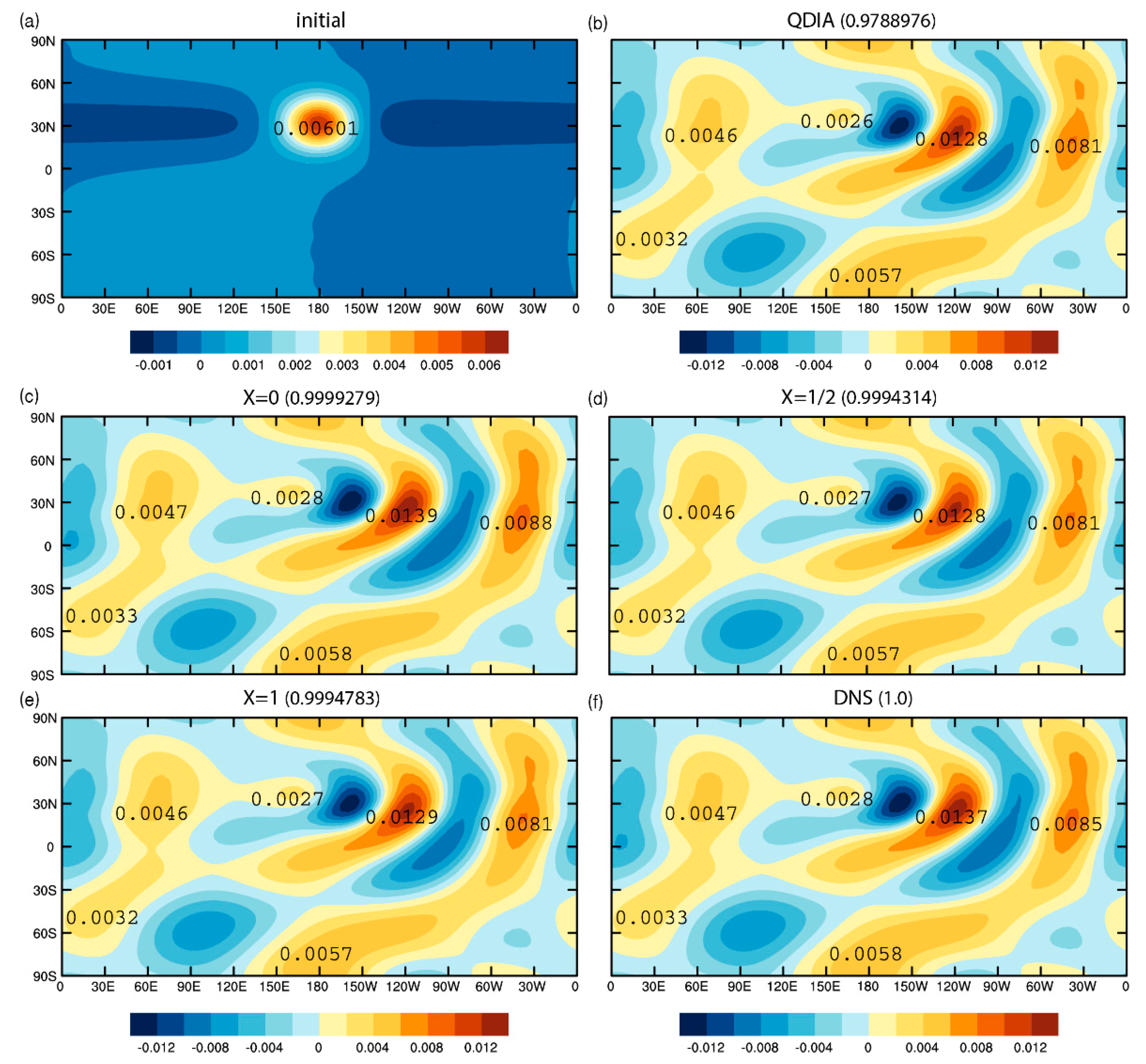
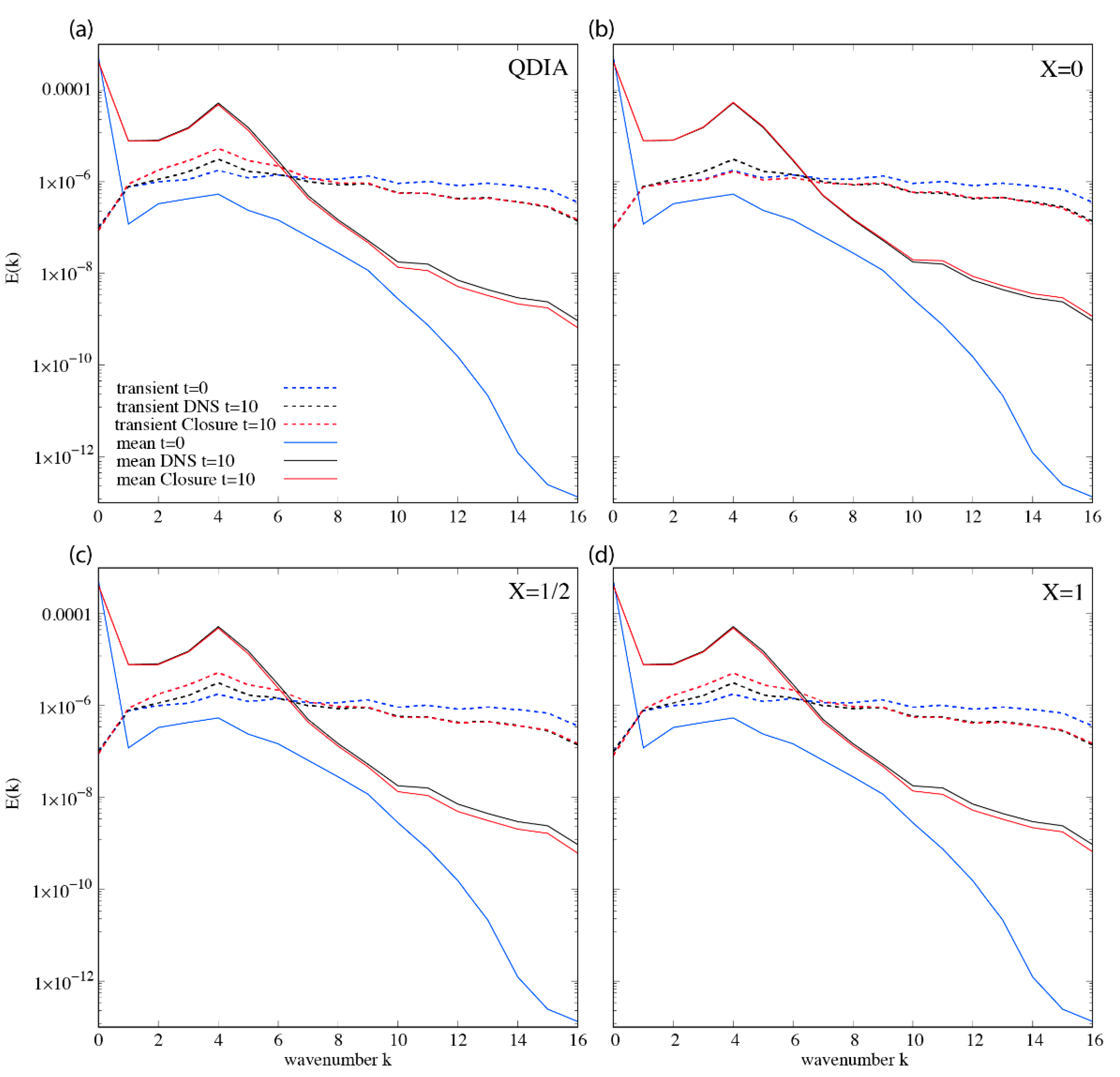
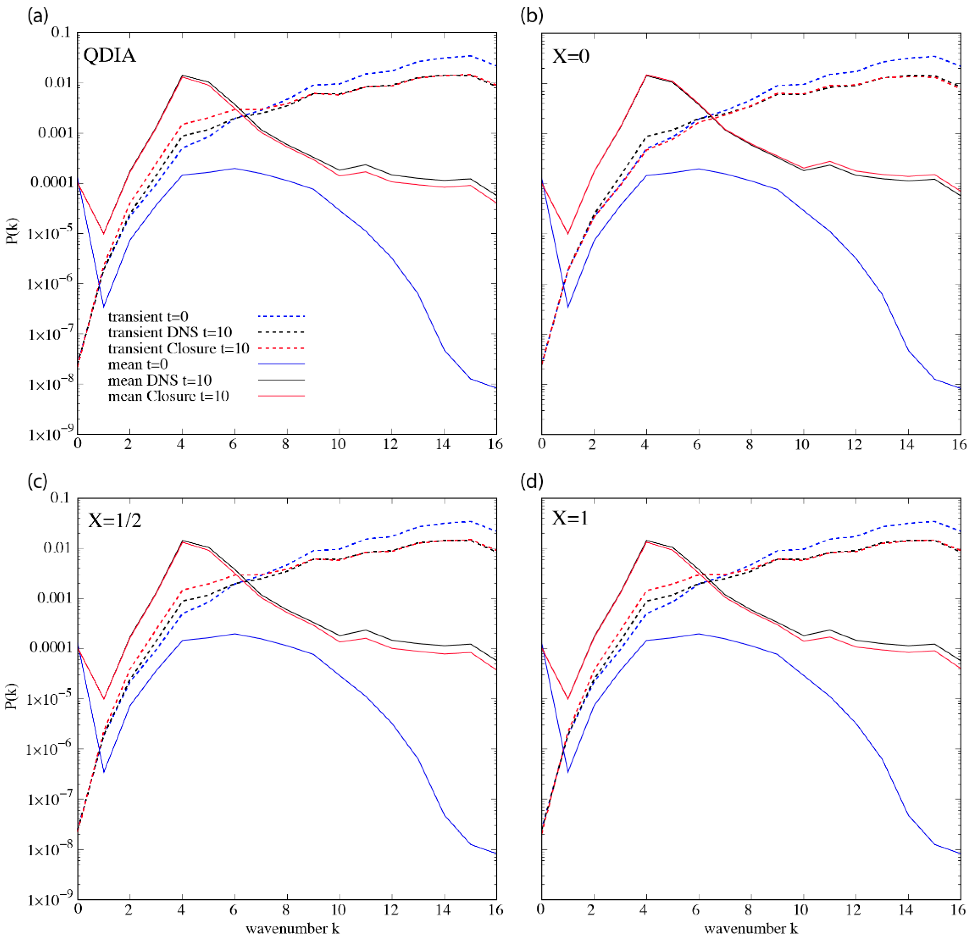
Table 1.
Initial conditions used in DNS and closure calculations.
Table 2.
Correlations of day 10 non-zonal streamfunction for closures with DNS.
Publisher’s Note: MDPI stays neutral with regard to jurisdictional claims in published maps and institutional affiliations. |
© 2022 by the authors. Licensee MDPI, Basel, Switzerland. This article is an open access article distributed under the terms and conditions of the Creative Commons Attribution (CC BY) license (https://creativecommons.org/licenses/by/4.0/).
Share and Cite
MDPI and ACS Style
Frederiksen, J.S.; O’Kane, T.J. Statistical Dynamics of Mean Flows Interacting with Rossby Waves, Turbulence, and Topography. Fluids 2022, 7, 200. https://0-doi-org.brum.beds.ac.uk/10.3390/fluids7060200
AMA Style
Frederiksen JS, O’Kane TJ. Statistical Dynamics of Mean Flows Interacting with Rossby Waves, Turbulence, and Topography. Fluids. 2022; 7(6):200. https://0-doi-org.brum.beds.ac.uk/10.3390/fluids7060200
Chicago/Turabian StyleFrederiksen, Jorgen S., and Terence J. O’Kane. 2022. "Statistical Dynamics of Mean Flows Interacting with Rossby Waves, Turbulence, and Topography" Fluids 7, no. 6: 200. https://0-doi-org.brum.beds.ac.uk/10.3390/fluids7060200