Analysis and Computations of Optimal Control Problems for Boussinesq Equations

Abstract

The main purpose of engineering applications for fluid with natural and mixed convection is to control or enhance the flow motion and the heat transfer. In this paper, we use mathematical tools based on optimal control theory to show the possibility of systematically controlling natural and mixed convection flows. We consider different control mechanisms such as distributed, Dirichlet, and Neumann boundary controls. We introduce mathematical tools such as functional spaces and their norms together with bilinear and trilinear forms that are used to express the weak formulation of the partial differential equations. For each of the three different control mechanisms, we aim to study the optimal control problem from a mathematical and numerical point of view. To do so, we present the weak form of the boundary value problem in order to assure the existence of solutions. We state the optimization problem using the method of Lagrange multipliers. In this paper, we show and compare the numerical results obtained by considering these different control mechanisms with different objectives.

1. Introduction

The optimization of complex systems in engineering is a crucial aspect that encourages and promotes research in the optimal control field. Optimization problems have three main ingredients: objectives, controls, and constraints. The first ingredient is the objective of interest in engineering applications, namely, flow matching, drag minimization, and enhancing or reducing turbulence. A quadratic functional minimization usually defines this objective. The controls can be chosen for large classes of design parameters. Examples are boundary controls such as injection or suction of fluid [1] and heating or cooling temperature controls [2,3,4], distributed controls such as heat sources or magnetic fields [5], and shape controls such as geometric domains [6]. Finally, a specific set of partial differential equations for the state variables defines the constraints. A typical optimization problem consists of finding state and control variables that minimize the objective functional and satisfy the imposed constraints [7]. In [7], the interested reader can find time-dependent and stochastic (input data polluted by random noise) analyses of optimal control theory that broaden the perspective of this work, here limited to stationary equations. Of course, the stochastic and optimal control time-dependent approach requires larger computational resources that severely limit real-life applications.

In this paper, we focus on engineering applications where fluid natural convection plays a main role. In these cases, buoyancy forces have a strong influence on the flow. Applications for natural convection optimal design are crucial in many contexts, ranging from semiconductor production processes, where buoyancy forces can control the crystal growth, to thermal hydraulics of lead-cooled fast reactors (LFR), where emergency cooling is guaranteed by natural convection. In the design of engineering devices such as heat exchangers, nuclear cores, and primary or secondary circuit pipes, optimization techniques can be used to achieve specified objectives such as desired wall temperatures or wall-normal heat fluxes, target mean temperatures, velocity profiles, or turbulence enhancements/reductions. The thermodynamic properties of lead allow a high level of natural circulation cooling in the primary system of an LFR. For core cooling, LFR design enhances strong natural circulation during plant operations and shutdown conditions [8]. Within this framework, we aim to study optimal control problems for mixed and natural convection.

In the past few years, the mathematical analysis of the optimal control of Navier–Stokes and energy equations has made considerable progress. The optimization of the heat transfer in forced convection flows can be found in many studies, mainly where the coupling between the Navier–Stokes and energy equations ignores density variations (see for example [2,4] and citations therein). In the case of natural or mixed convection flows, several authors have studied the mathematical analysis of the optimal control for the Oberbeck–Boussinesq system, focusing on stationary distributed and boundary thermal controls (see for example [3,5,9,10,11,12]). The solvability of the stationary boundary control problem for the Boussinesq equation is studied in [13,14], considering as boundary controls the velocity, the temperature, and the heat flux. Recently, new approaches to the study of the optimal control of Boussinesq equations have been proposed [15,16,17]. In [15], the solvability of an optimal control problem for steady non-isothermal incompressible creeping flows was proven. The temperature and the pressure in a flat portion of the local Lipschitz boundary played the role of controls. In [16], the optimal Neumann control problem for non-isothermal steady flows in low-concentration aqueous polymer solutions was considered, and sufficient conditions for the existence of optimal solutions were established. The problem of the optimal start control for unsteady Boussinesq equations was investigated in [17] to prove their solvability.

The main aim of this paper is to show the possibility of systematically controlling natural and mixed convection flows using mathematical tools based on optimal control theory. We consider three different control mechanisms: distributed, Dirichlet, and Neumann boundary controls. The solvability of the stationary optimal control problem for the Boussinesq equations has already been widely investigated in previous studies, considering as controls the forces and heat sources acting on the domain, together with the velocity, pressure, heat flux, and temperature on a portion of the boundary [3,5,9,10,11,12,13,14,15,16,17]. However, only a few studies show the numerical results of the optimal control problem for the Boussinesq equation and consider only a single control mechanism [2,11,14]. Thus, while the theoretical analysis of these control problems has been widely presented in previous studies, the implementation through an efficient numerical algorithm in a finite element code of the obtained optimality systems represents the novelty of this work. This paper aims to review the main thermal control mechanisms, showing and comparing the numerical results obtained for the different control mechanisms, objectives, and penalization parameters.

In Section 2, we first introduce the required mathematical tools such as functional spaces and their norms together with bilinear and trilinear forms that are used to express the weak formulation of the partial differential equations. In Section 3, the general forms of the optimal control problem and of the objective functional are presented. For each of the three different control mechanisms, we aim to study the optimal control problem from a mathematical point of view. To do so, we present the weak form of the boundary value problem, in order to prove the existence of solutions. We state the optimization problem and the existence of its solution using the method of Lagrange multipliers. Moreover, we present a numerical algorithm for each control type, in order to successfully solve the optimization system arising from the optimization problem. Numerical results are then presented in Section 4, considering the three thermal control mechanisms with different objectives for the temperature and velocity fields. The importance of the choice of the penalization parameter $\lambda$ is taken into account, and the results are discussed for different values of the penalization parameter.

2. Notation

We use the standard notation $H^s\left(\mathcal{O}\right)$ for a Sobolev space of order s with respect to the set $\mathcal{O}$, which can be the flow domain $\Omega \subset {\mathbb{R}}^n$, with $n=2,3$, or its boundary $\Gamma$. We remark that $H^0\left(\mathcal{O}\right)=L^2\left(\mathcal{O}\right)$. Corresponding Sobolev spaces of vector-valued functions are denoted by $H^s\left(\mathcal{O}\right)$. In particular, we denote the space ${\mathbf{H}}^1(\Omega )$ by $\{v_i\in L^2(\Omega )|\partial v_i/\partial x_j\in L^2(\Omega )\mathrm{for}i,j=1,\cdots ,n\}$ and the subspace ${\mathbf{H}}_{{\Gamma }_j}^1(\Omega )$ by $\left\{\mathbf{v}\in {\mathbf{H}}^1(\Omega )|\mathbf{v}=\mathbf{0}\mathrm{on}{\Gamma }_j\right\}$, where ${\Gamma }_j$ is a subset of $\Gamma$. In addition, we write ${\mathbf{H}}_0^1(\Omega )={\mathbf{H}}_{\Gamma }^1(\Omega )$. The dual space of ${\mathbf{H}}_{{\Gamma }_s}^1(\Omega )$ is denoted by ${\mathbf{H}}_{{\Gamma }_s}^{1*}(\Omega )$. In particular, the dual spaces of ${\mathbf{H}}^1(\Omega )$ and ${\mathbf{H}}_0^1(\Omega )$ are ${\mathbf{H}}^{1*}(\Omega )$ and ${\mathbf{H}}^{-1}(\Omega )$, respectively. We define the space of square integrable functions having zero mean over $\Omega$ as

$$L_0^2(\Omega )=\left\{q\in L^2(\Omega )|{\int }_{\Omega }qd\mathbf{x}=0\right\},$$

and the solenoidal spaces as

$$\mathbf{V}=\{\mathbf{v}\in {\mathbf{H}}^1(\Omega )|\nabla ·\mathbf{v}=0\},{\mathbf{V}}_0=\{\mathbf{v}\in {\mathbf{H}}_0^1(\Omega )|\nabla ·\mathbf{v}=0\}.$$

The norms of the functions belonging to $H^m\left(\mathcal{O}\right)$ are denoted by ${\parallel ·\parallel }_{m,\mathcal{O}}$. For $\left(fg\right)\in L^1\left(\mathcal{O}\right)$ and $(\mathbf{u}·\mathbf{v})\in L^1\left(\mathcal{O}\right)$, we define the scalar product as

$${(f,g)}_{\mathcal{O}}={\int }_{\mathcal{O}}fgd\mathbf{x},{(\mathbf{u},\mathbf{v})}_{\mathcal{O}}={\int }_{\mathcal{O}}\mathbf{u}·\mathbf{v}d\mathbf{x}.$$

Whenever possible, we will neglect the domain label. Thus, the inner product in $L^2(\Omega )$ and ${\mathbf{L}}^2(\Omega )$ are both denoted by $(·,·)$. This notation will also be employed to denote pairings between Sobolev spaces and their duals.

For the description of the Boussinesq system, we use the bilinear forms

$$\begin{array}{cccc}\hfill & a(\mathbf{u},\mathbf{v})={\int }_{\Omega }\nabla \mathbf{u}:\nabla \mathbf{v}d\mathbf{x}\hfill & \hfill & \forall \mathbf{u},\mathbf{v}\in {\mathbf{H}}^1(\Omega ),\hfill \end{array}$$

(1)

$$\begin{array}{cccc}\hfill & a(T,\theta )={\int }_{\Omega }\nabla T·\nabla \theta d\mathbf{x}\hfill & \hfill & \forall T,\theta \in H^1(\Omega ),\hfill \end{array}$$

(2)

$$\begin{array}{cccc}\hfill & b(\mathbf{u},q)=-{\int }_{\Omega }q\nabla ·\mathbf{u}d\mathbf{x}\hfill & \hfill & \forall q\in L_0^2(\Omega ),\forall \mathbf{u}\in {\mathbf{H}}^1(\Omega ),\hfill \end{array}$$

(3)

and the trilinear forms

$$\begin{array}{cccc}\hfill & c(\mathbf{w},\mathbf{u},\mathbf{v})={\int }_{\Omega }\mathbf{w}·\nabla \mathbf{u}·\mathbf{v}d\mathbf{x}\hfill & \hfill & \forall \mathbf{w},\mathbf{u},\mathbf{v}\in {\mathbf{H}}^1(\Omega ),\hfill \end{array}$$

(4)

$$\begin{array}{cccc}\hfill & c(\mathbf{w},T,\theta )={\int }_{\Omega }\mathbf{w}·\nabla T\theta d\mathbf{x}\hfill & \hfill & \forall \mathbf{w}\in {\mathbf{H}}^1(\Omega ),\forall T,\theta \in H^1(\Omega ).\hfill \end{array}$$

(5)

These forms are continuous [18]. Note that, for all $\mathbf{u}\in \mathbf{V}$, $\mathbf{v}\in {\mathbf{H}}^1(\Omega )$ and $T\in H^1(\Omega )$, we have $c(\mathbf{u},\mathbf{v},\mathbf{v})=0$ and $c(\mathbf{u},T,T)=0$.

3. Optimal Control of Boussinesq Equations

In this paper, we study optimal control problems for stationary incompressible flows in mixed or natural convection regimes. In these engineering applications, the dependence on the temperature field cannot be neglected in the Navier–Stokes equation. Thus, the temperature and velocity fields are mutually dependent through buoyancy forces and advection. These flows are defined by the following Boussinesq equations:

$$\begin{array}{cccc}\hfill & \nabla ·\mathbf{u}=0\hfill & \hfill & \mathrm{in}\Omega ,\hfill \end{array}$$

(6)

$$\begin{array}{cccc}\hfill & \mathbf{u}·\nabla \mathbf{u}+\nabla p-\nu \Delta \mathbf{u}=\mathbf{f}-\beta \mathbf{g}T\hfill & \hfill & \mathrm{in}\Omega ,\hfill \end{array}$$

(7)

$$\begin{array}{cccc}\hfill & \mathbf{u}·\nabla T-\alpha \Delta T=Q\hfill & \hfill & \mathrm{in}\Omega ,\hfill \end{array}$$

(8)

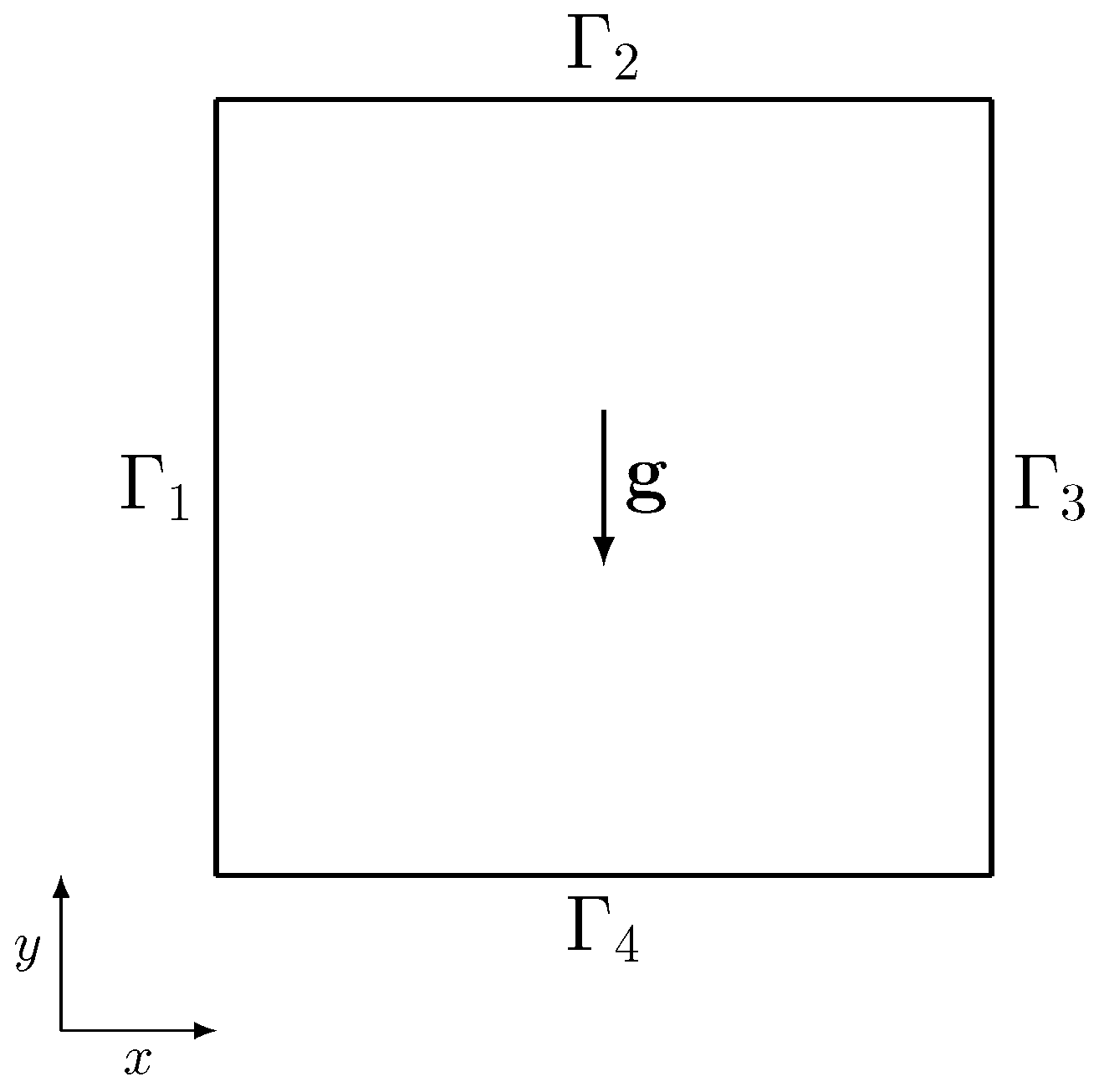
where $\Omega$ is a bounded open set in ${\mathbb{R}}^d$, $d=2$ or 3 with smoothing as necessary at boundary $\Gamma$. The operator $\Delta$ defines the Laplace operator $\nabla ·\nabla ={\nabla }^2=\Delta$. In (6)–(8), $\mathbf{u}$, p, and T denote the velocity, pressure, and temperature fields, while $\mathbf{f}$ is a body force, Q is a heat source, and $\mathbf{g}$ is the gravitational acceleration. The fluid thermal diffusivity, kinematic viscosity, and coefficient of expansion are defined by $\alpha$, $\nu$, and $\beta$, respectively. The system (6)–(8) is closed, with appropriate boundary conditions on $\partial \Omega$. For the velocity, we set Dirichlet boundary conditions, while for the temperature field we consider a mixed boundary condition defined as

$$\begin{array}{cccc}\hfill & \mathbf{u}=\mathbf{w}\hfill & \hfill & \mathrm{on}\partial \Omega ,\hfill \\ \hfill & T=g_t\hfill & \hfill & \mathrm{on}{\Gamma }_d,\hfill \\ \hfill & \alpha \nabla T·\mathbf{n}=g_{t,n}\hfill & \hfill & \mathrm{on}{\Gamma }_n.\hfill \end{array}$$

(9)

We denote by ${\Gamma }_d$ and ${\Gamma }_n$ the boundaries where Dirichlet and Neumann boundary conditions are applied, with ${\Gamma }_d\cup {\Gamma }_n=\Gamma =\partial \Omega$.

We formulate this control problem as a constrained minimization of the following objective functional:

$$\begin{array}{c}\hfill \mathcal{T}(\mathbf{u},T)=\frac{{\alpha }_u}{2}{\int }_{{\Omega }_d}|\mathbf{u}-{\mathbf{u}}_d{|}^{2}d\mathbf{x}+\frac{{\alpha }_T}{2}{\int }_{{\Omega }_d}{|T-T_d|}^{2}d\mathbf{x},\end{array}$$

(10)

subject to the Boussinesq Equations (6)–(8) imposed as constraints. In (10), the functions ${\mathbf{u}}_d$ and $T_d$ are the given desired velocity and temperature distributions. The terms in the functional (10) measure the $L^2(\Omega )$ distance between the velocity $\mathbf{u}$ and the target field ${\mathbf{u}}_d$ and/or between the temperature T and the target field $T_d$. The non-negative penalty parameters ${\alpha }_u$ and ${\alpha }_T$ can be used to change the relative importance of the terms appearing in the definition of the functional. If ${\alpha }_u=0$, we have as the objective a temperature matching case; if ${\alpha }_T=0$, we consider a velocity matching case.

The control can be a volumetric heat source, a boundary temperature, or a heat flux. In all these cases, the control has to be limited to avoid unbounded solutions. To do so, we can add a constraint limiting the value of the admissible control, or we can penalize the objective functional $\mathcal{T}$ by adding a regularization term. With this second approach, we do not need to impose any a priori constraints on the size of the control. Let c be the control belonging to a Hilbert space $H^s\left(\mathcal{O}\right)$. We can then define a cost functional

$$\begin{array}{c}\hfill \mathcal{J}(\mathbf{u},T,c)=\frac{{\alpha }_u}{2}{\int }_{{\Omega }_d}|\mathbf{u}-{\mathbf{u}}_d{|}^{2}d\mathbf{x}+\frac{{\alpha }_T}{2}{\int }_{{\Omega }_d}|T-T_d{|}^{2}d\mathbf{x}+{\lambda \left|\right|c\left|\right|}_{H^s\left(\mathcal{O}\right)},\end{array}$$

(11)

where the last term contains the $H^s\left(\mathcal{O}\right)$-norm of the control c penalized with a parameter $\lambda$. The value of the parameter $\lambda$ is used to change the relative importance of the objective and cost terms.

3.1. Dirichlet Boundary Control

In a Dirichlet boundary control problem, we aim to control the fluid state acting on the temperature on a portion of the boundary ${\Gamma }_c\subseteq {\Gamma }_d$. The boundary condition reported in (9) can be written in this case as

$$\begin{array}{cc}\hfill & \mathbf{u}=\mathbf{w}\mathrm{on}\partial \Omega ,T=g_t\mathrm{on}{\Gamma }_i,T=g_t+T_c\mathrm{on}{\Gamma }_c,\alpha \nabla T·\mathbf{n}=g_{t,n}\mathrm{on}{\Gamma }_n,\hfill \end{array}$$

(12)

where ${\Gamma }_i={\Gamma }_d\setminus {\Gamma }_c$. In (12), $g_t$, $g_{t,n}$, and $\mathbf{w}$ are given functions, while $T_c$ is the control. Thus, ${\Gamma }_c$ and ${\Gamma }_i$ denote the portions of ${\Gamma }_d$ where temperature control is and is not applied, respectively. By considering Equation (11) with $s=1$, the cost functional is given as follows:

$$\begin{array}{c}\hfill \mathcal{J}(\mathbf{u},T,T_c)=\frac{{\alpha }_u}{2}{\int }_{{\Omega }_d}|\mathbf{u}-{\mathbf{u}}_d{|}^{2}d\mathbf{x}+\frac{{\alpha }_T}{2}{\int }_{{\Omega }_d}|T-T_d{|}^{2}d\mathbf{x}+\frac{\lambda }{2}{\int }_{{\Gamma }_c}(|T_c{|}^2+|{\nabla }_s{T}_c{|}^2)d\mathbf{x},\end{array}$$

(13)

where ${\nabla }_s$ denotes the surface gradient operator, i.e., ${\nabla }_{s}f:=\nabla f-\mathbf{n}(\mathbf{n}·\nabla f)$. The cost contribution measures the $H^1\left({\Gamma }_c\right)$-norm of the control $T_c$.

3.1.1. Weak Formulation and Lagrange Multiplier Approach

The weak form of the boundary value problem (6)–(8) and (12) is given as follows: find $(\mathbf{u},p,T)\in {\mathbf{H}}^1(\Omega )\times L_0^2(\Omega )\times H^1(\Omega )$ such that

$$\begin{array}{cccc}\hfill & \nu a(\mathbf{u},\mathbf{v})+c(\mathbf{u},\mathbf{u},\mathbf{v})+b(\mathbf{v},p)=(\mathbf{f},\mathbf{v})-\beta (\mathbf{g}T,\mathbf{v})\hfill & \hfill & \forall \mathbf{v}\in {\mathbf{H}}_0^1(\Omega ),\hfill \\ \hfill & b(\mathbf{u},q)=0\hfill & \hfill & \forall q\in L_0^2(\Omega ),\hfill \\ \hfill & \alpha a(T,\phi )+c(\mathbf{u},T,\phi )=(Q,\phi )+{(g_{t,n},\phi )}_{{\Gamma }_n}\hfill & \hfill & \forall \phi \in H_{{\Gamma }_d}^1(\Omega ),\hfill \\ \hfill & {(T,s_T)}_{{\Gamma }_d}={(g_t,s_T)}_{{\Gamma }_d}+{(T_c,s_T)}_{{\Gamma }_c}\hfill & \hfill & \forall s_T\in H^{-1/2}\left({\Gamma }_d\right).\hfill \end{array}$$

(14)

The existence of the solution of the system (14) has been proved in [3]. Note that the normal heat flux on ${\Gamma }_d$ can be computed from T as

$$q_n{=-\alpha \nabla T·\mathbf{n}|}_{{\Gamma }_d}.$$

(15)

Now, we state the optimal control problem. We look for a $(\mathbf{u},p,T,T_c)\in {\mathbf{H}}^1(\Omega )\times L_0^2(\Omega )\times H^1(\Omega )\times H_0^1\left({\Gamma }_c\right)$ such that the cost functional (13) is minimized subject to the constraints (14). The admissible set of states and controls is

$$\begin{array}{c}\hfill \begin{array}{cc}\hfill {\mathcal{U}}_{ad}=\{& (\mathbf{u},p,T,T_c)\in {\mathbf{H}}^1(\Omega )\times L_0^2(\Omega )\times H^1(\Omega )\times H_0^1\left({\Gamma }_c\right):\hfill \\ & \mathcal{J}(\mathbf{u},T,T_c)<\infty \mathrm{and}\left(14\right)\mathrm{is}\mathrm{satified}.\}\hfill \end{array}\end{array}$$

(16)

Then, $(\widehat{\mathbf{u}},\widehat{p},\widehat{T},{\widehat{T}}_c)\in {\mathcal{U}}_{ad}$ is called an optimal solution if there exists $\epsilon >0$ such that

$$\begin{array}{c}\hfill \mathcal{J}(\widehat{\mathbf{u}},\widehat{p},\widehat{T},{\widehat{T}}_c,)\le \mathcal{J}(\mathbf{u},p,T,T_c)\forall (\mathbf{u},p,T,T_c)\in {\mathcal{U}}_{ad}\mathrm{satisfying}\\ \hfill \parallel \mathbf{u}-\widehat{\mathbf{u}}{\parallel }_1+\parallel p-\widehat{p}{\parallel }_0+\parallel T-\widehat{T}{\parallel }_1+{\parallel T_c-{\widehat{T}}_c\parallel }_{1,{\Gamma }_c}<\epsilon \end{array}$$

(17)

The existence of at least one optimal solution $(\widehat{\mathbf{u}},\widehat{p},\widehat{T},{\widehat{T}}_c)\in {\mathcal{U}}_{ad}$ was proven in [3].

We use the method of Lagrange multipliers to turn the constrained optimization problem (16) into an unconstrained one. We first show that suitable Lagrange multipliers exist. We summarize all the equations and the functional in two mappings and study their differential properties. It is convenient to define the following functional spaces:

$$\begin{array}{cc}\hfill & {\mathbf{B}}_1={\mathbf{H}}^1(\Omega )\times L_0^2(\Omega )\times H^1(\Omega )\times H_0^1\left({\Gamma }_c\right)\times H^{-\frac{1}{2}}\left({\Gamma }_d\right),\hfill \end{array}$$

(18)

$$\begin{array}{cc}\hfill & {\mathbf{B}}_2={\mathbf{H}}^{-1}(\Omega )\times L_0^2(\Omega )\times H_{{\Gamma }_i}^{1*}(\Omega )\times H^{\frac{1}{2}}\left({\Gamma }_d\right),\hfill \end{array}$$

(19)

$$\begin{array}{cc}\hfill & {\mathbf{B}}_3={\mathbf{H}}_0^1(\Omega )\times L_0^2(\Omega )\times H^1(\Omega )\times H_0^1\left({\Gamma }_c\right)\times H^{-\frac{1}{2}}\left({\Gamma }_d\right).\hfill \end{array}$$

(20)

Let $M:{\mathbf{B}}_1\to {\mathbf{B}}_2$ denote the generalized constraint equations, namely, $M\left(\mathbf{z}\right)$ = $\mathbf{l}$ for $\mathbf{z}=(\mathbf{u},p,T,T_c,q_n)\in {\mathbf{B}}_1$ and $\mathbf{l}=({\mathbf{l}}_1,l_2,l_3,l_4)$$\in {\mathbf{B}}_2$ if and only if

$$\begin{array}{cccc}\hfill & \nu a(\mathbf{u},\mathbf{v})+c(\mathbf{u},\mathbf{u},\mathbf{v})+b(\mathbf{v},p)-(\mathbf{f},\mathbf{v})+\beta (\mathbf{g}T,\mathbf{v})=({\mathbf{l}}_1,\mathbf{v})\hfill & \hfill & \forall \mathbf{v}\in {\mathbf{H}}_0^1(\Omega ),\hfill \\ \hfill & b(\mathbf{u},q)=(l_2,q)\hfill & \hfill & \forall q\in L_0^2(\Omega ),\hfill \\ \hfill & \alpha a(T,\phi )+c(\mathbf{u},T,\phi )-(Q,\phi )-{(g_{t,n},\phi )}_{{\Gamma }_n}-{(q_n,\phi )}_{{\Gamma }_c}=(l_3,\phi )\hfill & \hfill & \forall \phi \in H_{{\Gamma }_i}^1(\Omega ),\hfill \\ \hfill & {(T,s_T)}_{{\Gamma }_d}-{(g_t,s_T)}_{{\Gamma }_d}-{(T_c,s_T)}_{{\Gamma }_c}={(l_4,s_T)}_{{\Gamma }_d}\hfill & \hfill & \forall s_T\in H^{-1/2}\left({\Gamma }_d\right).\hfill \end{array}$$

(21)

Thus, the constraint (14) can be expressed as $M\left(\mathbf{z}\right)=\mathbf{0}$. Let $(\widehat{\mathbf{u}},\widehat{p},\widehat{T},{\widehat{T}}_c)\in {\mathbf{H}}^1(\Omega )\times L_0^2(\Omega )\times H^1(\Omega )\times H_0^1\left({\Gamma }_c\right)$ denote an optimal solution in the sense of (17). Then, consider the nonlinear operator $N:{\mathbf{B}}_1\to \mathbb{R}\times {\mathbf{B}}_2$ defined by

$$N(\mathbf{u},p,T,T_c,q_n)=\left(\begin{array}{c}\mathcal{J}(\mathbf{u},T,T_c)-\mathcal{J}(\widehat{\mathbf{u}},\widehat{T},{\widehat{T}}_c)\\ M(\mathbf{u},p,T,T_c,q_n)\end{array}\right).$$

(22)

Given $\mathbf{z}=(\mathbf{u},p,T,T_c,q_n)\in {\mathbf{B}}_1$, the operator $M^{\prime }\left(\mathbf{z}\right):{\mathbf{B}}_3\to {\mathbf{B}}_2$ may be defined as $M^{\prime }\left(\mathbf{z}\right)·\tilde{\mathbf{z}}=\tilde{\mathbf{l}}$ for $\tilde{\mathbf{z}}=(\tilde{\mathbf{u}},\tilde{p},\tilde{T},{\tilde{T}}_c,{\tilde{q}}_n)\in {\mathbf{B}}_3$ and $\tilde{\mathbf{l}}=({\tilde{\mathbf{l}}}_1,{\tilde{l}}_2,{\tilde{l}}_3,{\tilde{l}}_4)\in {\mathbf{B}}_2$ if and only if

$$\begin{array}{cccc}\hfill & \nu a(\tilde{\mathbf{u}},\mathbf{v})+c(\tilde{\mathbf{u}},\mathbf{u},\mathbf{v})+c(\mathbf{u},\tilde{\mathbf{u}},\mathbf{v})+b(\mathbf{v},\tilde{p})+\beta (\mathbf{g}\tilde{T},\mathbf{v})=({\tilde{\mathbf{l}}}_1,\mathbf{v})\hfill & \hfill & \forall \mathbf{v}\in {\mathbf{H}}_0^1(\Omega ),\hfill \\ \hfill & b(\tilde{\mathbf{u}},q)=({\tilde{l}}_2,q)\hfill & \hfill & \forall q\in L_0^2(\Omega ),\hfill \\ \hfill & \alpha a(\tilde{T},\phi )+c(\tilde{\mathbf{u}},T,\phi )+c(\mathbf{u},\tilde{T},\phi )-{({\tilde{q}}_n,\phi )}_{{\Gamma }_c}=({\tilde{l}}_3,\phi )\hfill & \hfill & \forall \phi \in H_{{\Gamma }_i}^1(\Omega ),\hfill \\ \hfill & {(\tilde{T},s_T)}_{{\Gamma }_d}-{({\tilde{T}}_c,s_T)}_{{\Gamma }_c}={({\tilde{l}}_4,s_T)}_{{\Gamma }_d}\hfill & \hfill & \forall s_T\in H^{-1/2}\left({\Gamma }_d\right).\hfill \end{array}$$

(23)

The operator $N^{\prime }\left(\mathbf{z}\right):{\mathbf{B}}_3\to \mathbb{R}\times {\mathbf{B}}_2$ may be defined as $N^{\prime }\left(\mathbf{z}\right)·\tilde{\mathbf{z}}=(\tilde{a},\tilde{\mathbf{l}})$ for $\tilde{a}\in \mathbb{R}$ if and only if

$$\begin{array}{cc}\hfill & {\alpha }_u{(\mathbf{u}-{\mathbf{u}}_d,\tilde{\mathbf{u}})}_{{\Omega }_d}+{\alpha }_T{(T-T_d,\tilde{T})}_{{\Omega }_d}+\lambda {(T_c,{\tilde{T}}_c)}_{{\Gamma }_c}+\hfill \\ & +\lambda {({\nabla }_s{T}_c,{\nabla }_s{\tilde{T}}_c)}_{{\Gamma }_c}=\tilde{a}\hfill \\ \hfill & \nu a(\tilde{\mathbf{u}},\mathbf{v})+c(\tilde{\mathbf{u}},\mathbf{u},\mathbf{v})+c(\mathbf{u},\tilde{\mathbf{u}},\mathbf{v})+b(\mathbf{v},\tilde{p})+\beta (\mathbf{g}\tilde{T},\mathbf{v})=({\tilde{\mathbf{l}}}_1,\mathbf{v})\hfill & \hfill & \forall \mathbf{v}\in {\mathbf{H}}_0^1(\Omega ),\hfill \\ \hfill & b(\tilde{\mathbf{u}},q)=({\tilde{l}}_2,q)\hfill & \hfill & \forall q\in L_0^2(\Omega ),\hfill \\ \hfill & \alpha a(\tilde{T},\phi )+c(\tilde{\mathbf{u}},T,\phi )+c(\mathbf{u},\tilde{T},\phi )-{({\tilde{q}}_n,\phi )}_{{\Gamma }_c}=({\tilde{l}}_3,\phi )\hfill & \hfill & \forall \phi \in H_{{\Gamma }_i}^1(\Omega ),\hfill \\ \hfill & {(\tilde{T},s_T)}_{{\Gamma }_d}-{({\tilde{T}}_c,s_T)}_{{\Gamma }_c}={({\tilde{l}}_4,s_T)}_{{\Gamma }_d}\hfill & \hfill & \forall s_T\in H^{-1/2}\left({\Gamma }_d\right).\hfill \end{array}$$

The differential operator $M^{\prime }$ is characterized by non-coercive elliptic equations. The advection terms in these equations are driven by the velocity field $\mathbf{u}\in {\mathbf{H}}^1(\Omega )$. Thus, the existence result for this class of equations is not trivial and cannot be obtained in the Lax–Milgram setting. However, by using a Leray–Schauder topological degree argument, we can introduce the following statements.

Let $\Omega \subset {\mathbb{R}}^n$ be a bounded open subset with boundary $\Gamma$. Let ${\Gamma }_d\subset \Gamma$ be a set with positive measure and ${\Gamma }_n\subseteq \Gamma \setminus {\Gamma }_d$. Consider

$$\begin{array}{cc}\hfill -\nabla ·(A^T\nabla y)+(\mathbf{u}·\nabla )y+by=f& \mathrm{in}\Omega ,\hfill \\ \hfill y=y_1& \mathrm{on}{\Gamma }_d,\hfill \\ \hfill A^T\nabla y·\mathbf{n}=y_n& \mathrm{on}{\Gamma }_n,\hfill \end{array}$$

(24)

with $b\in L^{n_{*}/2}(\Omega ),b\ge 0$ a.e. on $\Omega$, $\mathbf{u}\in {\mathbf{L}}^{n_{*}}(\Omega )$, and $f\in H_{{\Gamma }_D}^{1*}(\Omega )$, where $n_{*}=n$ when $n\ge 3$, $n_{*}\in ]2,\infty [$ when $n=2$. Based on the Leray–Schauder topological degree argument in [19], if A is a function which satisfies these two properties and:

• $\exists {\alpha }_A>0$ such that $A\left(x\right)\xi ·\xi \ge {\alpha }_A{\left|\xi \right|}^2$ for a.e. $x\in \Omega$ and for all $\xi \in {\mathbb{R}}^n$;
• $\exists {\Lambda }_A>0$ such that $\left|A\left(x\right)\right|\le {\Lambda }_A$ for a.e. $x\in \Omega$;

then, there exists a unique solution $y\in H^1(\Omega )$ of (24).

Furthermore, let ${\mathbf{z}}_0\in {\mathbf{B}}_{\mathbf{1}}$. Then we have that the operator $M^{\prime }\left({\mathbf{z}}_0\right)$ has closed range in ${\mathbf{B}}_{\mathbf{2}}$ and the operator $N^{\prime }\left({\mathbf{z}}_0\right)$ has closed range but is not in $\mathbb{R}\times {\mathbf{B}}_{\mathbf{2}}$. This allows us to find the Lagrange multipliers and the final optimality system. Let $\widehat{\mathbf{z}}=(\widehat{\mathbf{u}},\widehat{p},\widehat{T},{\widehat{T}}_c,{\widehat{q}}_n)\in {\mathbf{H}}^1(\Omega )\times L_0^2(\Omega )\times H^1(\Omega )\times H_0^1\left({\Gamma }_c\right)\times H^{-1/2}\left({\Gamma }_c\right)$ denote an optimal solution in the sense of (17). Then, there exists a nonzero Lagrange multiplier $(\Lambda ,{\widehat{\mathbf{u}}}_a,{\widehat{p}}_a,{\widehat{T}}_a,{\widehat{q}}_a)\in \mathbb{R}\times {\mathbf{B}}_2^{*}$ satisfying the Euler equations

$$\Lambda {\mathcal{J}}^{\prime }(\widehat{\mathbf{u}},\widehat{T},{\widehat{T}}_c)·\tilde{\mathbf{z}}+\langle ({\widehat{\mathbf{u}}}_a,{\widehat{p}}_a,{\widehat{T}}_a,{\widehat{q}}_a),M^{\prime }\left(\widehat{\mathbf{z}}\right)·\tilde{\mathbf{z}}\rangle =0,\forall \tilde{\mathbf{z}}\in {\mathbf{B}}_3,$$

(25)

where $\langle ·,·\rangle$ denotes the duality pairing between ${\mathbf{B}}_2$ and ${\mathbf{B}}_2^{*}$. For details on all the theoretical procedure regarding the existence of the Lagrange multipliers, the interested reader can consult [20].

3.1.2. The Optimality System

Now, we derive the optimality system using (25), and we drop the $\left(\widehat{·}\right)$ notation for the optimal solution. The Euler Equation (25) are equivalent to

$$\begin{array}{cc}\hfill & {\alpha }_u\Lambda {(\mathbf{u}-{\mathbf{u}}_d,\tilde{\mathbf{u}})}_{{\Omega }_d}+{\alpha }_T\Lambda {(T-T_d,\tilde{T})}_{{\Omega }_d}+\Lambda \lambda {(T_c,{\tilde{T}}_c)}_{{\Gamma }_c}+\Lambda \lambda {({\nabla }_s{T}_c,{\nabla }_s{\tilde{T}}_c)}_{{\Gamma }_c}+\hfill \\ \hfill & +b(\tilde{\mathbf{u}},p_a)+\nu a(\tilde{\mathbf{u}},{\mathbf{u}}_a)+c(\tilde{\mathbf{u}},\mathbf{u},{\mathbf{u}}_a)+b({\mathbf{u}}_a,\tilde{p})+c(\mathbf{u},\tilde{\mathbf{u}},{\mathbf{u}}_a)+\beta (\mathbf{g}\tilde{T},{\mathbf{u}}_a)+\hfill \\ \hfill & +\alpha a(\tilde{T},T_a)+c(\tilde{\mathbf{u}},T,T_a)+c(\mathbf{u},\tilde{T},T_a)-{({\tilde{q}}_n,T_a)}_{{\Gamma }_c}+{(\tilde{T},q_a)}_{{\Gamma }_d}-{({\tilde{T}}_c,q_a)}_{{\Gamma }_c}=0.\hfill \end{array}$$

(26)

By extracting the terms involved in the same variation and setting $\Lambda =-1$, we obtain the following equations:

$$\begin{array}{cc}\hfill & \nu a(\tilde{\mathbf{u}},{\mathbf{u}}_a)+c(\mathbf{u},\tilde{\mathbf{u}},{\mathbf{u}}_a)+c(\tilde{\mathbf{u}},\mathbf{u},{\mathbf{u}}_a)+b(\tilde{\mathbf{u}},p_a)=\hfill \\ \hfill & ={\alpha }_u{(\mathbf{u}-{\mathbf{u}}_d,\tilde{\mathbf{u}})}_{{\Omega }_d}-c(\tilde{\mathbf{u}};T,T_a)\hfill & \hfill & \forall \tilde{\mathbf{u}}\in {\mathbf{H}}_0^1(\Omega ),\hfill \\ \hfill & b({\mathbf{u}}_a,\tilde{p})=0\hfill & \hfill & \forall \tilde{p}\in L_0^2(\Omega ),\hfill \\ \hfill & \alpha a(\tilde{T},T_a)+c(\mathbf{u},\tilde{T},T_a)+{(\tilde{T},q_a)}_{{\Gamma }_c}=\hfill \\ \hfill & =-(\beta \mathbf{g}\tilde{T},{\mathbf{u}}_a)+{\alpha }_T{(T-T_d,\tilde{T})}_{{\Omega }_d}\hfill & \hfill & \forall \tilde{T}\in H_{{\Gamma }_i}^1(\Omega ),\hfill \\ \hfill & {(T_a,{\tilde{q}}_n)}_{{\Gamma }_c}=0,\hfill & \hfill & \forall {\tilde{q}}_n\in H^{-1/2}\left({\Gamma }_c\right),\hfill \end{array}$$

(27)

and the control equation

$$\begin{array}{cc}\hfill & \lambda {(T_c,{\tilde{T}}_c)}_{{\Gamma }_c}+\lambda {({\nabla }_s{T}_c,{\nabla }_s{\tilde{T}}_c)}_{{\Gamma }_c}+{(q_a,{\tilde{T}}_c)}_{{\Gamma }_c}=0\forall {\tilde{T}}_c\in H_0^1\left({\Gamma }_c\right),\hfill \end{array}$$

(28)

with $q_a=-\alpha \nabla T_a{·\mathbf{n}|}_{{\Gamma }_c}\mathrm{on}{\Gamma }_c$. The necessary conditions for an optimum are that Equations (14) and (27) are satisfied. This system of equations is called the optimality system. By applying integration by parts, it is easy to show that the system constitutes a weak formulation of the boundary value problem for the state equations

$$\begin{array}{cc}\hfill & \mathbf{u}·\nabla \mathbf{u}+\nabla p-\nu \Delta \mathbf{u}=\mathbf{f}-\beta \mathbf{g}T,\hfill \\ \hfill & \nabla ·\mathbf{u}=0,\hfill \\ \hfill & \mathbf{u}·\nabla T-\alpha \Delta T=Q,\hfill \\ \hfill & {\mathbf{u}=\mathbf{w}\mathrm{on}\Gamma ,\alpha \nabla T·\mathbf{n}|}_{{\Gamma }_n}=g_{t,n}\mathrm{on}{\Gamma }_n,T=g_t\mathrm{on}{\Gamma }_i,T=g_t+T_c\mathrm{on}{\Gamma }_c,\hfill \end{array}$$

(29)

the adjoint equations

$$\begin{array}{cc}\hfill & {\mathbf{u}}_a·{(\nabla \mathbf{u})}^T-\mathbf{u}·\nabla {\mathbf{u}}_a+\nabla p_a-\nu \Delta {\mathbf{u}}_a=-T\nabla T_a+{\alpha }_u(\mathbf{u}-{\mathbf{u}}_d),\hfill \\ \hfill & \nabla ·{\mathbf{u}}_a=0,\hfill \\ \hfill & -\alpha \Delta T_a-\mathbf{u}·\nabla T_a=-\beta \mathbf{g}·{\mathbf{u}}_a+{\alpha }_T(T-T_d),\hfill \\ \hfill & {\mathbf{u}}_a=0\mathrm{on}\Gamma ,\nabla T_a{·\mathbf{n}|}_{{\Gamma }_n}=0\mathrm{on}{\Gamma }_n,T_a=0\mathrm{on}{\Gamma }_d,\hfill \end{array}$$

(30)

and the control equation

$$\begin{array}{cc}\hfill & -{\Delta }_s{T}_c+T_c-\frac{\alpha \nabla T_a{·\mathbf{n}|}_{{\Gamma }_c}}{\lambda }=0\mathrm{on}{\Gamma }_c,\hfill \\ \hfill & T_c=0\mathrm{on}\partial {\Gamma }_c,\hfill \end{array}$$

(31)

where ${\Delta }_s$ denotes the surface Laplacian. The optimality system in the strong form consists of the Boussinesq system (29), the adjoint of the Boussinesq Equation (30), and the control Equation (31).

3.1.3. Numerical Algorithm

The optimality system consists of three groups of equations: the state Equation (14), the adjoint state Equation (27), and the optimality conditions for $T_c$ (28). Due to the nonlinearity and large dimension of this system, a one-shot solver cannot be implemented. We may construct an iterative method to iterate among the three groups of equations so that at each iteration we are dealing with a smaller-sized system of equations. We consider a gradient method for the solution of the optimality problem, and the gradient of the functional is determined with the help of the solution of the adjoint system.

Let us consider the gradient method for the following minimization problem: find $T_c\in H_0^1\left({\Gamma }_c\right)$ such that $\mathcal{F}\left(T_c\right):=\mathcal{J}(\mathbf{u}\left(T_c\right),T\left(T_c\right),T_c)$ is minimized. Given $T_c^{\left(0\right)}$, we can define the sequence

$$T_c^{(n+1)}=T_c^{\left(n\right)}-{\rho }^{\left(n\right)}\frac{d\mathcal{F}\left(T_c^{\left(n\right)}\right)}{d{T}_c^{\left(n\right)}},$$

(32)

recursively, where ${\rho }^{\left(n\right)}$ is a variable step size. Let ${\widehat{T}}_c$ be a solution of the minimization problem. Thus, the following necessary condition holds

$$\frac{d\mathcal{F}\left({\widehat{T}}_c\right)}{d{\widehat{T}}_c}=\frac{d\mathcal{J}(\mathbf{u}\left({\widehat{T}}_c\right),T\left({\widehat{T}}_c\right),{\widehat{T}}_c)}{d{\widehat{T}}_c}=0,$$

(33)

and at the optimum state the equality $T_c^{(n+1)}=T_c^{\left(n\right)}$ holds. For each fixed $T_c$, the Gâteaux derivative $(d\mathcal{F}\left(T_c\right)/d{T}_c)·{\tilde{T}}_c$ for every direction ${\tilde{T}}_c\in H^1\left({\Gamma }_c\right)$ may be computed as

$$\frac{d\mathcal{F}\left(T_c\right)}{d{T}_c}·{\tilde{T}}_c=\lambda {({\nabla }_s{T}_c,{\nabla }_s{\tilde{T}}_c)}_{{\Gamma }_c}+\lambda {(T_c,{\tilde{T}}_c)}_{{\Gamma }_c}+{({\tilde{T}}_c,q_a)}_{{\Gamma }_c},$$

(34)

or

$$\frac{d\mathcal{F}\left(T_c\right)}{d{T}_c}=-\lambda {\Delta }_s{T}_c+\lambda T_c+q_a.$$

(35)

Therefore, by combining (32) and (35), we implemented the following optimization algorithm.

(a)

Initial step:

• choose tolerance $\tau$ and $T_c^{\left(0\right)}$; set $n=0$ and ${\rho }^{\left(0\right)}=1$;
• solve for $({\mathbf{u}}^{\left(0\right)},p^{\left(0\right)},T^{\left(0\right)})$ from (14) with $T_c=T_c^{\left(0\right)}$;
• evaluate ${\mathcal{J}}^{\left(0\right)}=\mathcal{J}({\mathbf{u}}^{\left(0\right)},T^{\left(0\right)},T_c^{\left(0\right)})$ using (13).

(b)

Main loop:

• set $n=n+1$;
• solve for $({\mathbf{u}}_a^{\left(n\right)},p_a^{\left(n\right)},T_a^{\left(n\right)})$ from (27);
• solve for $T_c^{\left(n\right)}$ from

  $$\begin{array}{c}\hfill T_c^{\left(n\right)}=T_c^{(n-1)}-{\rho }^{\left(n\right)}\left(-{\Delta }_s{T}_c^{(n-1)}+T_c^{(n-1)}+\frac{\alpha }{\lambda }\nabla T_a^{\left(n\right)}{·\mathbf{n}|}_{{\Gamma }_c}\right),\end{array}$$

  (36)

  or

  $$\begin{array}{cc}\hfill -{\Delta }_s{T}_c^{\left(n\right)}+T_c^{\left(n\right)}=& -{\Delta }_s{T}_c^{(n-1)}+T_c^{(n-1)}-{\rho }^{\left(n\right)}(-{\Delta }_s{T}_c^{(n-1)}+T_c^{(n-1)}+\hfill \\ & +\frac{\alpha }{\lambda }\nabla T_a^{\left(n\right)}{·\mathbf{n}|}_{{\Gamma }_c});\hfill \end{array}$$

  (37)
• solve for $({\mathbf{u}}^{\left(n\right)},p^{\left(n\right)},T^{\left(n\right)})$ from (14) with $T_c=T_c^{\left(n\right)}$;
• evaluate ${\mathcal{J}}^{\left(n\right)}=\mathcal{J}({\mathbf{u}}^{\left(n\right)},T^{\left(n\right)},T_c^{\left(n\right)})$ using (13);

  (i)

  if ${\mathcal{J}}^{\left(n\right)}>{\mathcal{J}}^{(n-1)}$, set ${\rho }^{\left(n\right)}=0.5{\rho }^{\left(n\right)}$ and go to step (b) 3.;

  (ii)

  if ${\mathcal{J}}^{\left(n\right)}<{\mathcal{J}}^{(n-1)}$, set ${\rho }^{(n+1)}=1$ and go to step (b) 1.;

  (iii)

  if $|{\mathcal{J}}^{\left(n\right)}-{\mathcal{J}}^{(n-1)}|/|{\mathcal{J}}^{\left(n\right)}|<\tau$ stop.

In this algorithm, we propose two different methods, given by (36) and (37), for the control update. With the method in (37), we enforce the belonging of $T_c$ to $H_0^1\left({\Gamma }_c\right)$ and we give more regularity to the control. The convergence of the algorithm was proven in [3]. The finite element discretization of the optimality system and an estimation of the approximation error were analyzed in [11].

3.2. Neumann Boundary Control

In a Neumann boundary control problem, we aim to control the state by acting on the heat flux on a portion of the boundary ${\Gamma }_c\subseteq {\Gamma }_n$. The general boundary conditions reported in (9) can be written in this case as

$$\begin{array}{cc}\hfill & \mathbf{u}=\mathbf{w}\mathrm{on}\partial \Omega ,T=g_t\mathrm{on}{\Gamma }_d,\alpha \nabla T·\mathbf{n}=g_{t,n}\mathrm{on}{\Gamma }_i,\alpha \nabla T·\mathbf{n}=h\mathrm{on}{\Gamma }_c,\hfill \end{array}$$

(38)

where ${\Gamma }_i={\Gamma }_n\setminus {\Gamma }_c$. In (12), $g_t$, $g_{t,n}$, and $\mathbf{w}$ are given functions, while h is the control. Thus, ${\Gamma }_i$ and ${\Gamma }_c$ denote the portions of ${\Gamma }_n$ where the control is applied or not, respectively.

The cost functional is given as follows:

$$\begin{array}{c}\hfill \mathcal{J}(\mathbf{u},T,h)=\frac{{\alpha }_u}{2}{\int }_{{\Omega }_d}|\mathbf{u}-{\mathbf{u}}_d{|}^{2}d\mathbf{x}+\frac{{\alpha }_T}{2}{\int }_{{\Omega }_d}|T-T_d{|}^{2}d\mathbf{x}+\frac{\lambda }{2}{\int }_{{\Gamma }_c}{|h|}^{2}d\mathbf{x}.\end{array}$$

(39)

The cost contribution measures the $L^2\left({\Gamma }_c\right)$-norm of the control h.

3.2.1. Weak Formulation and Lagrange Multiplier Approach

The weak form of the boundary value problem (6)–(8) and (38) is given as follows: find $(\mathbf{u},p,T)\in {\mathbf{H}}^1(\Omega )\times L_0^2(\Omega )\times H^1(\Omega )$ such that

$$\begin{array}{cccc}\hfill & \nu a(\mathbf{u},\mathbf{v})+c(\mathbf{u},\mathbf{u},\mathbf{v})+b(\mathbf{v},p)=(\mathbf{f},\mathbf{v})-\beta (\mathbf{g}T,\mathbf{v})\hfill & \hfill & \forall \mathbf{v}\in {\mathbf{H}}_0^1(\Omega ),\hfill \\ \hfill & b(\mathbf{u},q)=0\hfill & \hfill & \forall q\in L_0^2(\Omega ),\hfill \\ \hfill & \alpha a(T,\phi )+c(\mathbf{u},T,\phi )=(Q,\phi )+{(g_{t,n},\phi )}_{{\Gamma }_i}+{(h,\phi )}_{{\Gamma }_c}\hfill & \hfill & \forall \phi \in H_{{\Gamma }_d}^1(\Omega ).\hfill \end{array}$$

(40)

The existence of the solution of the system (40) was proved in [9] (see Preposition 2.3).

Now, we state the optimal control problem: we look for a $(\mathbf{u},p,T,h)\in {\mathbf{H}}^1(\Omega )\times L_0^2(\Omega )\times H^1(\Omega )\times L^2\left({\Gamma }_c\right)$ such that the cost functional (39) is minimized subject to the constraints (40). The admissible set of states and controls is

$$\begin{array}{c}\hfill \begin{array}{cc}\hfill {\mathcal{U}}_{ad}=\{& (\mathbf{u},p,T,h)\in {\mathbf{H}}^1(\Omega )\times L_0^2(\Omega )\times H^1(\Omega )\times L^2\left({\Gamma }_c\right):\hfill \\ & \mathcal{J}(\mathbf{u},T,h)<\infty \mathrm{and}\left(40\right)\mathrm{is}\mathrm{satified}.\}\hfill \end{array}\end{array}$$

(41)

Then, $(\widehat{\mathbf{u}},\widehat{p},\widehat{T},\widehat{h})\in {\mathcal{U}}_{ad}$ is called an optimal solution if there exists $\epsilon >0$ such that

$$\begin{array}{c}\hfill \mathcal{J}(\widehat{\mathbf{u}},\widehat{p},\widehat{T},\widehat{h})\le \mathcal{J}(\mathbf{u},p,T,h)\forall (\mathbf{u},p,T,h)\in {\mathcal{U}}_{ad}\mathrm{satisfying}\\ \hfill \parallel \mathbf{u}-\widehat{\mathbf{u}}{\parallel }_1+\parallel p-\widehat{p}{\parallel }_0+\parallel T-\widehat{T}{\parallel }_1+{\parallel h-\widehat{h}\parallel }_{0,{\Gamma }_c}<\epsilon .\end{array}$$

(42)

The existence of at least one optimal solution $(\widehat{\mathbf{u}},\widehat{p},\widehat{T},\widehat{h})\in {\mathcal{U}}_{ad}$ was proved in [9].

In addition, for the Neumann control, we consider all the constraint equations and the functional to study their differential properties. We define the following functional spaces:

$$\begin{array}{cc}\hfill & {\mathbf{B}}_1={\mathbf{H}}^1(\Omega )\times L_0^2(\Omega )\times H^1(\Omega )\times L^2\left({\Gamma }_c\right),\hfill \end{array}$$

(43)

$$\begin{array}{cc}\hfill & {\mathbf{B}}_2={\mathbf{H}}^{-1}(\Omega )\times L_0^2(\Omega )\times H_{{\Gamma }_d}^{1*}(\Omega ),\hfill \end{array}$$

(44)

$$\begin{array}{cc}\hfill & {\mathbf{B}}_3={\mathbf{H}}_0^1(\Omega )\times L_0^2(\Omega )\times H_{{\Gamma }_d}^1(\Omega )\times L^2\left({\Gamma }_c\right).\hfill \end{array}$$

(45)

Let $M:{\mathbf{B}}_1\to {\mathbf{B}}_2$ denote the generalized constraint equations, namely, $M\left(\mathbf{z}\right)=\mathbf{l}$ for $\mathbf{z}=(\mathbf{u},p,T,h)\in {\mathbf{B}}_1$ and $\mathbf{l}=({\mathbf{l}}_1,l_2,l_3)$$\in {\mathbf{B}}_2$ if and only if

$$\begin{array}{cccc}\hfill & \nu a(\mathbf{u},\mathbf{v})+c(\mathbf{u},\mathbf{u},\mathbf{v})+b(\mathbf{v},p)-(\mathbf{f},\mathbf{v})+\beta (\mathbf{g}T,\mathbf{v})=({\mathbf{l}}_1,\mathbf{v})\hfill & \hfill & \forall \mathbf{v}\in {\mathbf{H}}_0^1(\Omega ),\hfill \\ \hfill & b(\mathbf{u},q)=(l_2,q)\hfill & \hfill & \forall q\in L_0^2(\Omega ),\hfill \\ \hfill & \alpha a(T,\phi )+c(\mathbf{u},T,\phi )-(Q,\phi )-{(g_{t,n},\phi )}_{{\Gamma }_i}-{(h,\phi )}_{{\Gamma }_c}=(l_3,\phi )\hfill & \hfill & \forall \phi \in H_{{\Gamma }_d}^1(\Omega ).\hfill \end{array}$$

(46)

Thus, the constraints (40) can be expressed as $M\left(\mathbf{z}\right)=\mathbf{0}$. Let $(\widehat{\mathbf{u}},\widehat{p},\widehat{T},\widehat{h})\in {\mathbf{H}}^1(\Omega )\times L_0^2(\Omega )\times H^1(\Omega )\times L^2\left({\Gamma }_c\right)$ denote an optimal solution in the sense of (42). Then, consider the nonlinear operator $N:{\mathbf{B}}_1\to \mathbb{R}\times {\mathbf{B}}_2$ defined by

$$N(\mathbf{u},p,T,h)=\left(\begin{array}{c}\mathcal{J}(\mathbf{u},T,h)-\mathcal{J}(\widehat{\mathbf{u}},\widehat{T},\widehat{h})\\ M(\mathbf{u},p,T,h)\end{array}\right).$$

(47)

Given $\mathbf{z}=(\mathbf{u},p,T,h)\in {\mathbf{B}}_1$, the operator $M^{\prime }\left(\mathbf{z}\right):{\mathbf{B}}_3\to {\mathbf{B}}_2$ may be defined as $M^{\prime }\left(\mathbf{z}\right)·\tilde{\mathbf{z}}=\tilde{\mathbf{l}}$ for $\tilde{\mathbf{z}}=(\tilde{\mathbf{u}},\tilde{p},\tilde{T},\tilde{h})\in {\mathbf{B}}_3$ and $\tilde{\mathbf{l}}=({\tilde{\mathbf{l}}}_1,{\tilde{l}}_2,{\tilde{l}}_3)\in {\mathbf{B}}_2$ if and only if

$$\begin{array}{cccc}\hfill & \nu a(\tilde{\mathbf{u}},\mathbf{v})+c(\tilde{\mathbf{u}},\mathbf{u},\mathbf{v})+c(\mathbf{u},\tilde{\mathbf{u}},\mathbf{v})+b(\mathbf{v},\tilde{p})+\beta (\mathbf{g}\tilde{T},\mathbf{v})=({\tilde{\mathbf{l}}}_1,\mathbf{v})\hfill & \hfill & \forall \mathbf{v}\in {\mathbf{H}}_0^1(\Omega ),\hfill \\ \hfill & b(\tilde{\mathbf{u}},q)=({\tilde{l}}_2,q)\hfill & \hfill & \forall q\in L_0^2(\Omega ),\hfill \\ \hfill & \alpha a(\tilde{T},\phi )+c(\tilde{\mathbf{u}},T,\phi )+c(\mathbf{u},\tilde{T},\phi )-{(\tilde{h},\phi )}_{{\Gamma }_c}=({\tilde{l}}_3,\phi )\hfill & \hfill & \forall \phi \in H_{{\Gamma }_d}^1(\Omega ).\hfill \end{array}$$

(48)

The operator $N^{\prime }\left(\mathbf{z}\right):{\mathbf{B}}_3\to \mathbb{R}\times {\mathbf{B}}_2$ may be defined as $N^{\prime }\left(\mathbf{z}\right)·\tilde{\mathbf{z}}=(\tilde{a},\tilde{\mathbf{l}})$ for $\tilde{a}\in \mathbb{R}$ if and only if

$$\begin{array}{cc}\hfill & {\alpha }_u{(\mathbf{u}-{\mathbf{u}}_d,\tilde{\mathbf{u}})}_{{\Omega }_d}+{\alpha }_T{(T-T_d,\tilde{T})}_{{\Omega }_d}+\lambda {(h,\tilde{h})}_{{\Gamma }_c}=\tilde{a}\hfill \\ \hfill & \nu a(\tilde{\mathbf{u}},\mathbf{v})+c(\tilde{\mathbf{u}},\mathbf{u},\mathbf{v})+c(\mathbf{u},\tilde{\mathbf{u}},\mathbf{v})+b(\mathbf{v},\tilde{p})+\beta (\mathbf{g}\tilde{T},\mathbf{v})=({\tilde{\mathbf{l}}}_1,\mathbf{v})\hfill & \hfill & \forall \mathbf{v}\in {\mathbf{H}}_0^1(\Omega ),\hfill \\ \hfill & b(\tilde{\mathbf{u}},q)=({\tilde{l}}_2,q)\hfill & \hfill & \forall q\in L_0^2(\Omega ),\hfill \\ \hfill & \alpha a(\tilde{T},\phi )+c(\tilde{\mathbf{u}},T,\phi )+c(\mathbf{u},\tilde{T},\phi )-{(\tilde{h},\phi )}_{{\Gamma }_c}=({\tilde{l}}_3,\phi )\hfill & \hfill & \forall \phi \in H_{{\Gamma }_d}^1(\Omega ).\hfill \end{array}$$

(49)

Let ${\mathbf{z}}_0\in {\mathbf{B}}_{\mathbf{1}}$. Then, we have that the operator $M^{\prime }\left({\mathbf{z}}_0\right)$ has closed range in ${\mathbf{B}}_{\mathbf{2}}$ and the operator $N^{\prime }\left({\mathbf{z}}_0\right)$ has closed range but is not in $\mathbb{R}\times {\mathbf{B}}_{\mathbf{2}}$. This follows standard techniques (see [21]). Therefore, let $\widehat{\mathbf{z}}=(\widehat{\mathbf{u}},\widehat{p},\widehat{T},\widehat{h})\in {\mathbf{H}}^1(\Omega )\times L_0^2(\Omega )\times H^1(\Omega )\times L^2\left({\Gamma }_c\right)$ denote an optimal solution satisfying (42). Then, there exists a nonzero Lagrange multiplier $(\Lambda ,{\widehat{\mathbf{u}}}_a,{\widehat{p}}_a,{\widehat{T}}_a)\in \mathbb{R}\times {\mathbf{B}}_2^{*}$ satisfying the Euler equations

$$\Lambda {\mathcal{J}}^{\prime }(\widehat{\mathbf{u}},\widehat{T},\widehat{h})·\tilde{\mathbf{z}}+\langle ({\widehat{\mathbf{u}}}_a,{\widehat{p}}_a,{\widehat{T}}_a),M^{\prime }\left(\widehat{\mathbf{z}}\right)·\tilde{\mathbf{z}}\rangle =0,\forall \tilde{\mathbf{z}}\in {\mathbf{B}}_3,$$

(50)

where $\langle ·,·\rangle$ denotes the duality pairing between ${\mathbf{B}}_2$ and ${\mathbf{B}}_2^{*}$.

3.2.2. The Optimality System

We drop the $\left(\widehat{·}\right)$ notation for the optimal solution and derive now the optimality system using (50). The Euler Equation (50) are equivalent to

$$\begin{array}{cc}\hfill & {\alpha }_u\Lambda {(\mathbf{u}-{\mathbf{u}}_d,\tilde{\mathbf{u}})}_{{\Omega }_d}+{\alpha }_T\Lambda {(T-T_d,\tilde{T})}_{{\Omega }_d}+\Lambda \lambda {(h,\tilde{h})}_{{\Gamma }_c}+b(\tilde{\mathbf{u}},p_a)+\nu a(\tilde{\mathbf{u}},{\mathbf{u}}_a)+\hfill \\ & +c(\tilde{\mathbf{u}},\mathbf{u},{\mathbf{u}}_a)+b({\mathbf{u}}_a,\tilde{p})+c(\mathbf{u},\tilde{\mathbf{u}},{\mathbf{u}}_a)+\beta (\mathbf{g}\tilde{T},{\mathbf{u}}_a)+\alpha a(\tilde{T},T_a)+\hfill \\ & +c(\tilde{\mathbf{u}},T,T_a)+c(\mathbf{u},\tilde{T},T_a)-{(\tilde{h},T_a)}_{{\Gamma }_c}=0.\hfill \end{array}$$

(51)

By extracting the terms involved in the same variation and setting $\Lambda =-1$, we obtain the following equations:

$$\begin{array}{cc}\hfill & \nu a(\tilde{\mathbf{u}},{\mathbf{u}}_a)+c(\mathbf{u},\tilde{\mathbf{u}},{\mathbf{u}}_a)+c(\tilde{\mathbf{u}},\mathbf{u},{\mathbf{u}}_a)+b(\tilde{\mathbf{u}},p_a)d=\hfill \\ \hfill & ={\alpha }_u{(\mathbf{u}-{\mathbf{u}}_d,\tilde{\mathbf{u}})}_{{\Omega }_d}-c(\tilde{\mathbf{u}};T,T_a)\hfill & \hfill & \forall \tilde{\mathbf{u}}\in {\mathbf{H}}_0^1(\Omega ),\hfill \\ \hfill & b({\mathbf{u}}_a,\tilde{p})=0\hfill & \hfill & \forall \tilde{p}\in L_0^2(\Omega ),\hfill \\ \hfill & \alpha a(\tilde{T},T_a)+c(\mathbf{u},\tilde{T},T_a)=-(\beta \mathbf{g}\tilde{T},{\mathbf{u}}_a)+{\alpha }_T{(T-T_d,\tilde{T})}_{{\Omega }_d}\hfill & \hfill & \forall \tilde{T}\in H_{{\Gamma }_d}^1(\Omega ),\hfill \end{array}$$

(52)

and the control equation

$$\begin{array}{ccc}\hfill \lambda {(h,\tilde{h})}_{{\Gamma }_c}+{(\tilde{h},T_a)}_{{\Gamma }_c}=0& \hfill & \hfill \forall \tilde{h}\in L^2\left({\Gamma }_c\right).\end{array}$$

(53)

The necessary conditions for an optimum are that Equations (40) and (52) are satisfied. This system of equations is called the optimality system. Integrations by parts may be used to show that the system constitutes a weak formulation of the boundary value problem

$$\begin{array}{cc}\hfill & \mathbf{u}·\nabla \mathbf{u}+\nabla p-\nu \Delta \mathbf{u}=\mathbf{f}-\beta \mathbf{g}T,\hfill \\ \hfill & \nabla ·\mathbf{u}=0,\hfill \\ \hfill & \mathbf{u}·\nabla T-\alpha \Delta T=Q,\hfill \\ \hfill & {\mathbf{u}=\mathbf{w}\mathrm{on}\Gamma ,\alpha \nabla T·\mathbf{n}|}_{{\Gamma }_i}=g_{t,n}\mathrm{on}{\Gamma }_i{,\alpha \nabla T·\mathbf{n}|}_{{\Gamma }_c}=h\mathrm{on}{\Gamma }_c,T=g_t\mathrm{on}{\Gamma }_d,\hfill \end{array}$$

(54)

the adjoint equations

$$\begin{array}{cc}\hfill & {\mathbf{u}}_a·{(\nabla \mathbf{u})}^T-\mathbf{u}·\nabla {\mathbf{u}}_a+\nabla p_a-\nu \Delta {\mathbf{u}}_a=-T\nabla T_a+{\alpha }_u(\mathbf{u}-{\mathbf{u}}_d),\hfill \\ \hfill & \nabla ·{\mathbf{u}}_a=0,\hfill \\ \hfill & -\alpha \Delta T_a-\mathbf{u}·\nabla T_a=-\beta \mathbf{g}·{\mathbf{u}}_a+{\alpha }_T(T-T_d),\hfill \\ \hfill & {\mathbf{u}}_a=0\mathrm{on}\Gamma ,\nabla T_a{·\mathbf{n}|}_{{\Gamma }_n}=0\mathrm{on}{\Gamma }_n,T_a=0\mathrm{on}{\Gamma }_d,\hfill \end{array}$$

(55)

and the control equation

$$h=-\frac{T_a}{\lambda }\mathrm{on}{\Gamma }_c.$$

(56)

The optimality system in the strong form consists of the Boussinesq system (54), the adjoint of Boussinesq Equation (55), and the control Equation (56).

3.2.3. Numerical Algorithm

We consider the gradient method for the following minimization problem: find $h\in L^2\left({\Gamma }_c\right)$ such that $\mathcal{F}\left(h\right):=\mathcal{J}\left(\mathbf{u}\right(h),T(h),h)$ is minimized. Given $h^{\left(0\right)}$, we can define the sequence

$$h^{(n+1)}=h^{\left(n\right)}-{\rho }^{\left(n\right)}\frac{d\mathcal{F}\left(h^{\left(n\right)}\right)}{d{h}^{\left(n\right)}},$$

(57)

recursively, where ${\rho }^{\left(n\right)}$ is a variable step size. For each fixed $T_c$, the Gâteaux derivative $(d\mathcal{F}\left(h\right)/dh)·\tilde{h}$ for every direction $\tilde{h}\in L^2\left({\Gamma }_c\right)$ may be computed as

$$\begin{array}{cc}\hfill & \frac{d\mathcal{F}\left(h\right)}{dh}·\tilde{h}=\lambda {(h,\tilde{h})}_{{\Gamma }_c}+{(\tilde{h},T_a)}_{{\Gamma }_c},\hfill \end{array}$$

(58)

or

$$\frac{d\mathcal{F}\left(h\right)}{dh}=h+\frac{T_a}{\lambda }.$$

(59)

The optimization algorithm is then given as follows

(a)

Initial step:

• choose tolerance $\tau$ and $h^{\left(0\right)}$; set $n=0$ and ${\rho }^{\left(0\right)}=1$;
• solve for $({\mathbf{u}}^{\left(0\right)},p^{\left(0\right)},T^{\left(0\right)})$ from (40) with $h=h^{\left(0\right)}$;
• evaluate ${\mathcal{J}}^{\left(0\right)}=\mathcal{J}({\mathbf{u}}^{\left(0\right)},T^{\left(0\right)},h^{\left(0\right)})$ using (39).

(b)

Main loop:

• set $n=n+1$;
• solve for $({\mathbf{u}}_a^{\left(n\right)},p_a^{\left(n\right)},T_a^{\left(n\right)})$ from (52);
• solve for $h^{\left(n\right)}$ from

  $$h^{\left(n\right)}=h^{(n-1)}-{\rho }^{\left(n\right)}\left(h^{(n-1)}+\frac{T_a^{\left(n\right)}}{\lambda }\right);$$

  (60)
• solve for $({\mathbf{u}}^{\left(n\right)},p^{\left(n\right)},T^{\left(n\right)})$ from (40) with $h=h^{\left(n\right)}$;
• evaluate ${\mathcal{J}}^{\left(n\right)}=\mathcal{J}({\mathbf{u}}^{\left(n\right)},T^{\left(n\right)},h^{\left(n\right)})$ using (39);

  (i)

  if ${\mathcal{J}}^{\left(n\right)}>{\mathcal{J}}^{(n-1)}$, set ${\rho }^{\left(n\right)}=0.5{\rho }^{\left(n\right)}$ and go to step (b) 3.;

  (ii)

  if ${\mathcal{J}}^{\left(n\right)}<{\mathcal{J}}^{(n-1)}$, set ${\rho }^{(n+1)}=1$ and go to step (b) 1.;

  (iii)

  if $|{\mathcal{J}}^{\left(n\right)}-{\mathcal{J}}^{(n-1)}|/|{\mathcal{J}}^{\left(n\right)}|<\tau$ stop.

3.3. Distributed Control

A distributed control problem aims to control the flow state using a heat source acting on the domain $\Omega$ as a control mechanism. In (8), the heat source Q is the control of the optimal control problem. The boundary conditions are those reported in (9), where $\mathbf{w}$, $g_t$, and $g_{t,n}$ are given functions. The cost functional is formulated as

$$\begin{array}{c}\hfill \mathcal{J}(\mathbf{u},T,Q)=\frac{{\alpha }_u}{2}{\int }_{{\Omega }_d}|\mathbf{u}-{\mathbf{u}}_d{|}^{2}d\mathbf{x}+\frac{{\alpha }_T}{2}{\int }_{{\Omega }_d}|T-T_d{|}^{2}d\mathbf{x}+\frac{\lambda }{2}{\int }_{\Omega }{|Q|}^{2}d\mathbf{x},\end{array}$$

(61)

where the cost contribution measures the $L^2(\Omega )$-norm of the control Q.

3.3.1. Weak Formulation and Lagrange Multiplier Approach

The weak form of the boundary value problem (6)–(9) is given as follows: find $(\mathbf{u},p,T)\in {\mathbf{H}}^1(\Omega )\times L_0^2(\Omega )\times H^1(\Omega )$ such that

$$\begin{array}{cccc}\hfill & \nu a(\mathbf{u},\mathbf{v})+c(\mathbf{u},\mathbf{u},\mathbf{v})+b(\mathbf{v},p)=(\mathbf{f},\mathbf{v})-\beta (\mathbf{g}T,\mathbf{v})\hfill & \hfill & \forall \mathbf{v}\in {\mathbf{H}}_0^1(\Omega ),\hfill \\ \hfill & b(\mathbf{u},q)=0\hfill & \hfill & \forall q\in L_0^2(\Omega ),\hfill \\ \hfill & \alpha a(T,\phi )+c(\mathbf{u},T,\phi )=(Q,\phi )+{(g_{t,n},\phi )}_{{\Gamma }_n}\hfill & \hfill & \forall \phi \in H_{{\Gamma }_d}^1(\Omega ).\hfill \end{array}$$

(62)

The existence of the solution of the system (62) can be proved as in [9].

We now state the optimal control problem. We look for a $(\mathbf{u}$, p, T, $Q)$$\in {\mathbf{H}}^1(\Omega )\times L_0^2(\Omega )\times H^1(\Omega )\times L^2(\Omega )$ such that the cost functional (61) is minimized subject to the constraints (62). The admissible set of states and controls is

$$\begin{array}{c}\hfill \begin{array}{cc}\hfill {\mathcal{U}}_{ad}=\{& (\mathbf{u},p,T,Q)\in {\mathbf{H}}^1(\Omega )\times L_0^2(\Omega )\times H^1(\Omega )\times L^2(\Omega ):\hfill \\ & \mathcal{J}(\mathbf{u},T,Q)<\infty \mathrm{and}\left(62\right)\mathrm{is}\mathrm{satified}.\}\hfill \end{array}\end{array}$$

(63)

Then $(\widehat{\mathbf{u}},\widehat{p},\widehat{T},\widehat{Q})\in {\mathcal{U}}_{ad}$ is called an optimal solution if there exists $\epsilon >0$ such that

$$\begin{array}{c}\hfill \mathcal{J}(\widehat{\mathbf{u}},\widehat{p},\widehat{T},\widehat{Q})\le \mathcal{J}(\mathbf{u},p,T,Q)\forall (\mathbf{u},p,T,Q)\in {\mathcal{U}}_{ad}\mathrm{satisfying}\\ \hfill \parallel \mathbf{u}-\widehat{\mathbf{u}}{\parallel }_1+\parallel p-\widehat{p}{\parallel }_0+\parallel T-\widehat{T}{\parallel }_1+{\parallel Q-\widehat{Q}\parallel }_0<\epsilon .\end{array}$$

(64)

The existence of at least one optimal solution $(\widehat{\mathbf{u}},\widehat{p},\widehat{T},\widehat{Q})\in {\mathcal{U}}_{ad}$ can be proved as in [9].

We define the following functional spaces:

$$\begin{array}{cc}\hfill & {\mathbf{B}}_1={\mathbf{H}}^1(\Omega )\times L_0^2(\Omega )\times H^1(\Omega )\times L^2(\Omega ),\hfill \end{array}$$

(65)

$$\begin{array}{cc}\hfill & {\mathbf{B}}_2={\mathbf{H}}^{-1}(\Omega )\times L_0^2(\Omega )\times H_{{\Gamma }_d}^{1*}(\Omega ),\hfill \end{array}$$

(66)

$$\begin{array}{cc}\hfill & {\mathbf{B}}_3={\mathbf{H}}_0^1(\Omega )\times L_0^2(\Omega )\times H_{{\Gamma }_d}^1(\Omega )\times L^2(\Omega ).\hfill \end{array}$$

(67)

Let $M:{\mathbf{B}}_1\to {\mathbf{B}}_2$ denote the generalized constraint equations, namely, $M\left(\mathbf{z}\right)=\mathbf{l}$ for $\mathbf{z}=(\mathbf{u},p,T,Q)\in {\mathbf{B}}_1$ and $\mathbf{l}=({\mathbf{l}}_1,l_2,l_3)$$\in {\mathbf{B}}_2$ if and only if

$$\begin{array}{cccc}\hfill & \nu a(\mathbf{u},\mathbf{v})+c(\mathbf{u},\mathbf{u},\mathbf{v})+b(\mathbf{v},p)-(\mathbf{f},\mathbf{v})+\beta (\mathbf{g}T,\mathbf{v})=({\mathbf{l}}_1,\mathbf{v})\hfill & \hfill & \forall \mathbf{v}\in {\mathbf{H}}_0^1(\Omega ),\hfill \\ \hfill & b(\mathbf{u},q)=(l_2,q)\hfill & \hfill & \forall q\in L_0^2(\Omega ),\hfill \\ \hfill & \alpha a(T,\phi )+c(\mathbf{u},T,\phi )-(Q,\phi )-{(g_{t,n},\phi )}_{{\Gamma }_n}=(l_3,\phi )\hfill & \hfill & \forall \phi \in H_{{\Gamma }_d}^1(\Omega ).\hfill \end{array}$$

(68)

Thus, the constraints (62) can be expressed as $M\left(\mathbf{z}\right)=\mathbf{0}$. Let $(\widehat{\mathbf{u}},\widehat{p},\widehat{T},\widehat{Q})\in {\mathbf{H}}^1(\Omega )\times L_0^2(\Omega )\times H^1(\Omega )\times L^2(\Omega )$ denote an optimal solution in the sense of (64). Then, consider the nonlinear operator $N:{\mathbf{B}}_1\to \mathbb{R}\times {\mathbf{B}}_2$ defined by

$$N(\mathbf{u},p,T,Q)=\left(\begin{array}{c}\mathcal{J}(\mathbf{u},T,Q)-\mathcal{J}(\widehat{\mathbf{u}},\widehat{T},\widehat{Q})\\ M(\mathbf{u},p,T,Q)\end{array}\right).$$

(69)

Given $\mathbf{z}=(\mathbf{u},p,T,Q)\in {\mathbf{B}}_1$, the operator $M^{\prime }\left(\mathbf{z}\right):{\mathbf{B}}_3\to {\mathbf{B}}_2$ may be defined as $M^{\prime }\left(\mathbf{z}\right)·\tilde{\mathbf{z}}=\tilde{\mathbf{l}}$ for $\tilde{\mathbf{z}}=(\tilde{\mathbf{u}},\tilde{p},\tilde{T},\tilde{Q})\in {\mathbf{B}}_3$ and $\tilde{\mathbf{l}}=({\tilde{\mathbf{l}}}_1,{\tilde{l}}_2,{\tilde{l}}_3)\in {\mathbf{B}}_2$ if and only if

$$\begin{array}{cccc}\hfill & \nu a(\tilde{\mathbf{u}},\mathbf{v})+c(\tilde{\mathbf{u}},\mathbf{u},\mathbf{v})+c(\mathbf{u},\tilde{\mathbf{u}},\mathbf{v})+b(\mathbf{v},\tilde{p})+\beta (\mathbf{g}\tilde{T},\mathbf{v})=({\tilde{\mathbf{l}}}_1,\mathbf{v})\hfill & \hfill & \forall \mathbf{v}\in {\mathbf{H}}_0^1(\Omega ),\hfill \\ \hfill & b(\tilde{\mathbf{u}},q)=({\tilde{l}}_2,q)\hfill & \hfill & \forall q\in L_0^2(\Omega ),\hfill \\ \hfill & \alpha a(\tilde{T},\phi )+c(\tilde{\mathbf{u}},T,\phi )+c(\mathbf{u},\tilde{T},\phi )-(\tilde{Q},\phi )=({\tilde{l}}_3,\phi )\hfill & \hfill & \forall \phi \in H_{{\Gamma }_d}^1(\Omega ).\hfill \end{array}$$

(70)

The operator $N^{\prime }\left(\mathbf{z}\right):{\mathbf{B}}_3\to \mathbb{R}\times {\mathbf{B}}_2$ may be defined as $N^{\prime }\left(\mathbf{z}\right)·\tilde{\mathbf{z}}=(\tilde{a},\tilde{\mathbf{l}})$ for $\tilde{a}\in \mathbb{R}$ if and only if

$$\begin{array}{cc}\hfill & {\alpha }_u{(\mathbf{u}-{\mathbf{u}}_d,\tilde{\mathbf{u}})}_{{\Omega }_d}+{\alpha }_T{(T-T_d,\tilde{T})}_{{\Omega }_d}+\lambda (Q,\tilde{Q})=\tilde{a}\hfill \\ \hfill & \nu a(\tilde{\mathbf{u}},\mathbf{v})+c(\tilde{\mathbf{u}},\mathbf{u},\mathbf{v})+c(\mathbf{u},\tilde{\mathbf{u}},\mathbf{v})+b(\mathbf{v},\tilde{p})+\beta (\mathbf{g}\tilde{T},\mathbf{v})=({\tilde{\mathbf{l}}}_1,\mathbf{v})\hfill & \hfill & \forall \mathbf{v}\in {\mathbf{H}}_0^1(\Omega ),\hfill \\ \hfill & b(\tilde{\mathbf{u}},q)=({\tilde{l}}_2,q)\hfill & \hfill & \forall q\in L_0^2(\Omega ),\hfill \\ \hfill & \alpha a(\tilde{T},\phi )+c(\tilde{\mathbf{u}},T,\phi )+c(\mathbf{u},\tilde{T},\phi )-(\tilde{Q},\phi )=({\tilde{l}}_3,\phi )\hfill & \hfill & \forall \phi \in H_{{\Gamma }_d}^1(\Omega ).\hfill \end{array}$$

(71)

Let ${\mathbf{z}}_0\in {\mathbf{B}}_{\mathbf{1}}$. We have that the operator $M^{\prime }\left({\mathbf{z}}_0\right)$ has closed range in ${\mathbf{B}}_{\mathbf{2}}$ and the operator $N^{\prime }\left({\mathbf{z}}_0\right)$ has closed range but is not in $\mathbb{R}\times {\mathbf{B}}_{\mathbf{2}}$ [21].

Similarly to the other controls presented in previous sections, let $\widehat{\mathbf{z}}=(\widehat{\mathbf{u}},\widehat{p},\widehat{T},\widehat{Q})\in {\mathbf{H}}^1(\Omega )\times L_0^2(\Omega )\times H^1(\Omega )\times L^2(\Omega )$ denote an optimal solution in the sense of (64). Then, there exists a nonzero Lagrange multiplier $(\Lambda ,{\widehat{\mathbf{u}}}_a,{\widehat{p}}_a,{\widehat{T}}_a)\in \mathbb{R}\times {\mathbf{B}}_2^{*}$ satisfying the Euler equations

$$\Lambda {\mathcal{J}}^{\prime }(\widehat{\mathbf{u}},\widehat{T},\widehat{Q})·\tilde{\mathbf{z}}+\langle ({\widehat{\mathbf{u}}}_a,{\widehat{p}}_a,{\widehat{T}}_a),M^{\prime }\left(\widehat{\mathbf{z}}\right)·\tilde{\mathbf{z}}\rangle =0\forall \tilde{\mathbf{z}}\in {\mathbf{B}}_3,$$

(72)

where $\langle ·,·\rangle$ denotes the duality pairing between ${\mathbf{B}}_2$ and ${\mathbf{B}}_2^{*}$. The interested reader can consult [21] on the existence of the Lagrange multiplier.

3.3.2. Optimality System

As in the previous case, we drop the $\left(\widehat{·}\right)$ notation for the optimal solution and derive the optimality system using the Euler Equation (72)

$$\begin{array}{cc}\hfill & {\alpha }_u\Lambda {(\mathbf{u}-{\mathbf{u}}_d,\tilde{\mathbf{u}})}_{{\Omega }_d}+{\alpha }_T\Lambda {(T-T_d,\tilde{T})}_{{\Omega }_d}+\Lambda \lambda (Q,\tilde{Q})+b(\tilde{\mathbf{u}},p_a)+\nu a(\tilde{\mathbf{u}},{\mathbf{u}}_a)+\hfill \\ \hfill & +c(\tilde{\mathbf{u}},\mathbf{u},{\mathbf{u}}_a)+b({\mathbf{u}}_a,\tilde{p})+c(\mathbf{u},\tilde{\mathbf{u}},{\mathbf{u}}_a)+\beta (\mathbf{g}\tilde{T},{\mathbf{u}}_a)+\alpha a(\tilde{T},T_a)+c(\tilde{\mathbf{u}},T,T_a)+\hfill \\ \hfill & +c(\mathbf{u},\tilde{T},T_a)-(\tilde{Q},T_a)=0.\hfill \end{array}$$

(73)

We extract the terms involved in the same variation, set $\Lambda =-1$, and obtain the following equations:

$$\begin{array}{cc}\hfill & \nu a(\tilde{\mathbf{u}},{\mathbf{u}}_a)+c(\mathbf{u},\tilde{\mathbf{u}},{\mathbf{u}}_a)+c(\tilde{\mathbf{u}},\mathbf{u},{\mathbf{u}}_a)+b(\tilde{\mathbf{u}},p_a)=\hfill \\ \hfill & ={\alpha }_u{(\mathbf{u}-{\mathbf{u}}_d,\tilde{\mathbf{u}})}_{{\Omega }_d}-c(\tilde{\mathbf{u}};T,T_a)\hfill & \hfill & \forall \tilde{\mathbf{u}}\in {\mathbf{H}}_0^1(\Omega ),\hfill \\ \hfill & b({\mathbf{u}}_a,\tilde{p})=0\hfill & \hfill & \forall \tilde{p}\in L_0^2(\Omega ),\hfill \\ \hfill & \alpha a(\tilde{T},T_a)+c(\mathbf{u},\tilde{T},T_a)=-(\beta \mathbf{g}\tilde{T},{\mathbf{u}}_a)+{\alpha }_T{(T-T_d,\tilde{T})}_{{\Omega }_d}\hfill & \hfill & \forall \tilde{T}\in H_{{\Gamma }_d}^1(\Omega ),\hfill \end{array}$$

(74)

and the control equation

$$\begin{array}{cc}\hfill & \lambda (Q,\tilde{Q})+(\tilde{Q},T_a)=0,\forall \tilde{Q}\in L^2(\Omega ).\hfill \end{array}$$

(75)

The necessary conditions for an optimum are defined by Equations (62) and (74). This system of equations is the optimality system. We can use integrations to show that the system constitutes a weak formulation of the boundary value problem for state equations

$$\begin{array}{cc}\hfill & \mathbf{u}·\nabla \mathbf{u}+\nabla p-\nu \Delta \mathbf{u}=\mathbf{f}-\beta \mathbf{g}T,\hfill \\ \hfill & \nabla ·\mathbf{u}=0,\hfill \\ \hfill & \mathbf{u}·\nabla T-\alpha \Delta T=Q,\hfill \\ \hfill & {\mathbf{u}=\mathbf{w}\mathrm{on}\Gamma ,\alpha \nabla T·\mathbf{n}|}_{{\Gamma }_n}=g_{t,n}\mathrm{on}{\Gamma }_n,T=g_t\mathrm{on}{\Gamma }_d,\hfill \end{array}$$

(76)

the adjoint equations

$$\begin{array}{cc}\hfill & {\mathbf{u}}_a·{(\nabla \mathbf{u})}^T-\mathbf{u}·\nabla {\mathbf{u}}_a+\nabla p_a-\nu \Delta {\mathbf{u}}_a=-T\nabla T_a+{\alpha }_u(\mathbf{u}-{\mathbf{u}}_d),\hfill \\ \hfill & \nabla ·{\mathbf{u}}_a=0,\hfill \\ \hfill & -\alpha \Delta T_a-\mathbf{u}·\nabla T_a=-\beta \mathbf{g}·{\mathbf{u}}_a+{\alpha }_T(T-T_d),\hfill \\ \hfill & {\mathbf{u}}_a=0\mathrm{on}\Gamma ,\nabla T_a{·\mathbf{n}|}_{{\Gamma }_n}=0\mathrm{on}{\Gamma }_n,T_a=0\mathrm{on}{\Gamma }_d,\hfill \end{array}$$

(77)

and the control equation

$$Q=-\frac{T_a}{\lambda }\mathrm{in}\Omega .$$

(78)

Therefore, the optimality system in the strong form consists of the Boussinesq system (76), the adjoint of Boussinesq Equation (77), and the control Equation (78).

3.3.3. Numerical Algorithm

Let us consider the gradient method for the following minimization problem: find $Q\in L^2(\Omega )$ such that $\mathcal{F}\left(Q\right):=\mathcal{J}\left(\mathbf{u}\right(Q),T(Q),Q)$ is minimized. Given $Q^{\left(0\right)}$, we can define the sequence

$$Q^{(n+1)}=Q^{\left(n\right)}-{\rho }^{\left(n\right)}\frac{d\mathcal{F}\left(Q^{\left(n\right)}\right)}{d{Q}^{\left(n\right)}},$$

(79)

recursively, where ${\rho }^{\left(n\right)}$ is a variable step size. Let ${\widehat{Q}}_c$ be a solution of the minimization problem. Thus, at the optimum $d\mathcal{F}\left(\widehat{Q}\right)/d\widehat{Q}=0$ and $Q^{(n+1)}=Q^{\left(n\right)}$. The Gâteaux derivative $(d\mathcal{F}\left(Q\right)/dQ)·\tilde{Q}$ for every direction $\tilde{Q}\in L^2(\Omega )$ may be computed as

$$\begin{array}{cc}\hfill & \frac{d\mathcal{F}\left(Q\right)}{dQ}·\tilde{Q}=\lambda (Q,\tilde{Q})+(\tilde{Q},T_a).\hfill \end{array}$$

(80)

Thus, the Gâteaux derivative may be computed as

$$\frac{d\mathcal{F}\left(Q\right)}{dQ}=Q+\frac{T_a}{\lambda }.$$

(81)

The optimization algorithm is then given as follows.

(a)

Initial step:

• choose tolerance $\tau$ and $Q^{\left(0\right)}$; set $n=0$ and ${\rho }^{\left(0\right)}=1$;
• solve for $({\mathbf{u}}^{\left(0\right)},p^{\left(0\right)},T^{\left(0\right)})$ from (62) with $Q=Q^{\left(0\right)}$;
• evaluate ${\mathcal{J}}^{\left(0\right)}=\mathcal{J}({\mathbf{u}}^{\left(0\right)},T^{\left(0\right)},Q^{\left(0\right)})$ using (61).

(b)

Main loop:

• set $n=n+1$;
• solve for $({\mathbf{u}}_a^{\left(n\right)},p_a^{\left(n\right)},T_a^{\left(n\right)})$ from (74);
• solve for $Q^{\left(n\right)}$ from

  $$Q^{\left(n\right)}=Q^{(n-1)}-{\rho }^{\left(n\right)}\left(Q^{(n-1)}+\frac{T_a^{\left(n\right)}}{\lambda }\right);$$

  (82)
• solve for $({\mathbf{u}}^{\left(n\right)},p^{\left(n\right)},T^{\left(n\right)})$ from (40) with $Q=Q^{\left(n\right)}$;
• evaluate ${\mathcal{J}}^{\left(n\right)}=\mathcal{J}({\mathbf{u}}^{\left(n\right)},T^{\left(n\right)},Q^{\left(n\right)})$ using (39);

  (i)

  if ${\mathcal{J}}^{\left(n\right)}>{\mathcal{J}}^{(n-1)}$, set ${\rho }^{\left(n\right)}=0.5{\rho }^{\left(n\right)}$ and go to step (b) 3.;

  (ii)

  if ${\mathcal{J}}^{\left(n\right)}<{\mathcal{J}}^{(n-1)}$, set ${\rho }^{(n+1)}=1$ and go to step (b) 1.;

  (iii)

  if $|{\mathcal{J}}^{\left(n\right)}-{\mathcal{J}}^{(n-1)}|/|{\mathcal{J}}^{\left(n\right)}|<\tau$ stop.

4. Numerical Results

In this section, we report some numerical results obtained by using the mathematical models shown in the previous sections. The main difference between the three control problems is in the nature of the control equations. For Neumann and distributed controls, the control equation is an algebraic equation that states that the control is proportional to the adjoint temperature (see Equations (56) and (78)). In contrast, when we have a Dirichlet boundary control, the control equation is a partial differential equation with the normal adjoint temperature gradient as source term, as reported in (31). Thus, the adjoint temperature $T_a$ plays a key role in all three control mechanisms, as does the regularization parameter $\lambda$ that appears in the denominator of the source terms. The adjoint temperature $T_a$ depends on the objectives of the velocity and temperature fields. When the objective relates to the temperature field, the dependence is direct through the term ${\alpha }_T(T-T_d)$ appearing on the right-hand side of the adjoint temperature Equations (27), (52), and (74). If the objective relates to the velocity field, the control mechanism is indirect, since the term ${\alpha }_u(\mathbf{u}-{\mathbf{u}}_d)$ acts as a source in the adjoint velocity equation. In turn, the adjoint velocity appears in the source term of the adjoint temperature $\beta \mathbf{g}·{\mathbf{u}}_a$.

The geometry considered for all the simulations is a square cavity with $L=0.01\mathrm{m}$. The domain $\Omega =[0,L]\times [0,L]\in {\mathbb{R}}^2$ is shown in Figure 1. We consider liquid lead with the properties reported in

Table 1. Boussinesq control: physical properties employed for the numerical simulations.

Property	Symbol	Value	Units
Viscosity	$\mu$	$0.00181$	$\mathrm{Pa}\mathrm{s}$
Density	$\rho$	$\mathrm{10,340}$	${\mathrm{kg}/\mathrm{m}}^3$
Thermal conductivity	$\lambda$	$10.72$	W/(mK)
Specific heat	c	$145.75$	J/(kgK)
Coefficient of expansion	$\beta$	$2.5684\times {10}^{-4}$	${\mathrm{K}}^{-1}$

. We discretize the numerical problem in a finite element framework, and we consider a $20\times 20$ uniform quadrangular mesh formed by biquadratic elements. The simulations were performed using the in-house finite element multigrid code FEMuS developed at the University of Bologna [22]. The code is based on a C++ main program that handles several external open-source libraries such as the MPI and PETSc libraries.

4.1. Dirichlet Boundary Control

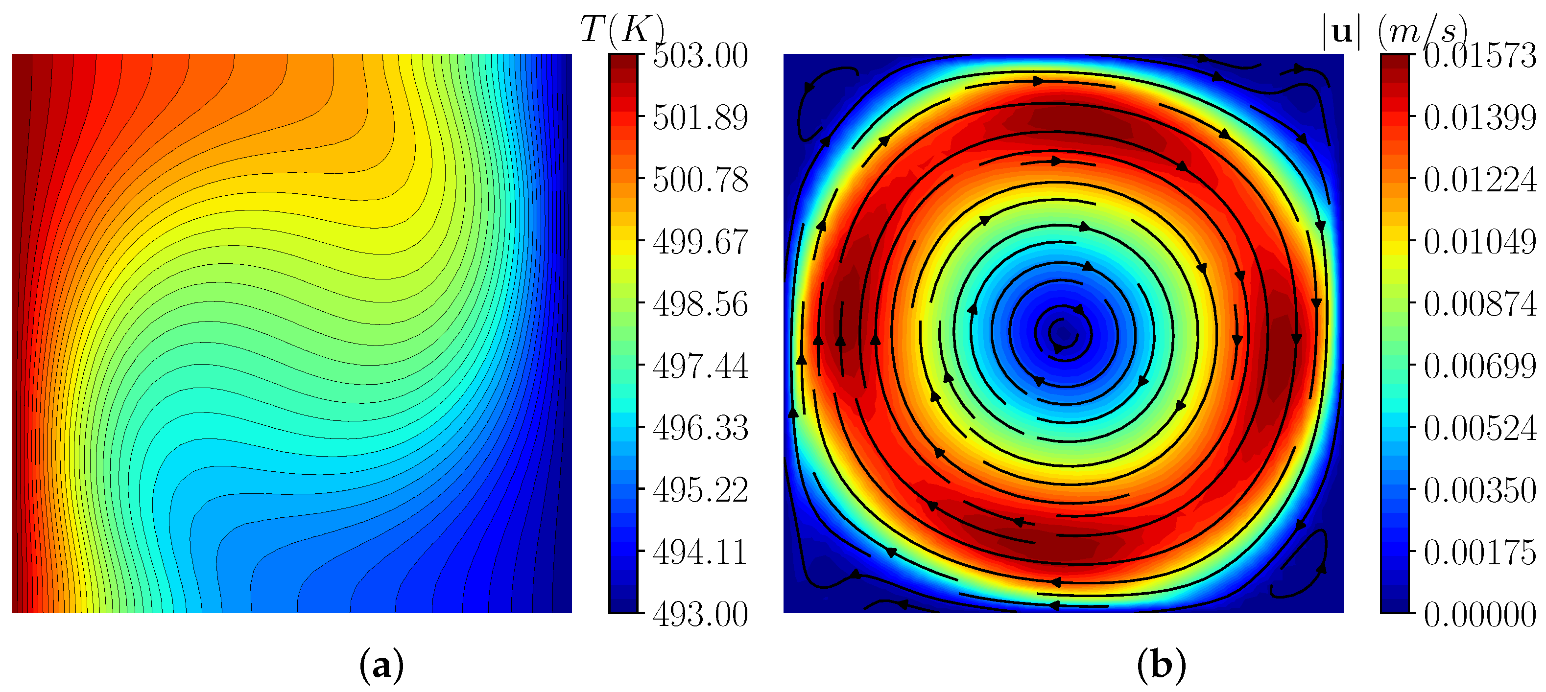
We now show the numerical results for the Dirichlet boundary control. The boundary conditions are reported in (12), where ${\Gamma }_d={\Gamma }_1\cup {\Gamma }_3$, ${\Gamma }_i={\Gamma }_3$, ${\Gamma }_c={\Gamma }_1$ and ${\Gamma }_n={\Gamma }_2\cup {\Gamma }_4$. We set $\mathbf{f}=\mathbf{0}$ and $Q=0$ in (14), and ${\mathbf{g}}_u=\mathbf{0}$, $g_{t,n}=0$, $g_t=493\mathrm{K}$ on ${\Gamma }_3$, and $g_t=503\mathrm{K}$ on ${\Gamma }_1$ in (12). For the reference case, we set $T_c^{\left(0\right)}=0$. Then, on ${\Gamma }_c={\Gamma }_1$ we have $T^{\left(0\right)}=g_t$. In Figure 2a,b, we show the temperature and velocity contours, respectively, of the numerical solution when the control algorithm is not applied. Lead flows in the cavity and forms a clockwise vortex due to buoyancy forces caused by the heated cavity wall. The bulk velocity is $U_b=0.008765\mathrm{m}/\mathrm{s}$. The Richardson number, computed as $Ri=gL\Delta T\beta /U_b^2$, is equal to $3.28$. The Grashof number is $Gr=RiR{e}^2=8.2\times {10}^5$. Lastly, the Rayleigh number is given by $Ra=GrPr=2\times {10}^4$. The results shown in Figure 2 follow the typical features of temperature and velocity profiles for $Ra\approx {10}^4$, i.e., isotherms departing from the vertical position with the formation of a central elliptic clockwise vortex [23].

4.1.1. Temperature Matching Case

Firstly, we aim to test the optimization algorithm with a temperature matching case. Let (13) be the objective functional with ${\alpha }_u=0$, ${\alpha }_T=1$, and ${\Omega }_d=[0.45L;0.55L]\times [0.75L;0.85L]$. The region ${\Omega }_d$ is indicated in Figure 3a. We set $T_d=450\mathrm{K}$. Then, in ${\Omega }_d$ we aim at obtaining cooler fluid than in the reference case reported in Figure 2a. We consider four different values of the regularization parameter $\lambda$, namely, ${10}^{-5},{10}^{-6},{10}^{-7}$, and ${10}^{-8}$. The reference objective functional is ${\mathcal{J}}^{\left(0\right)}=0.001250$. For the numerical simulations, we use the algorithm for Dirichlet boundary problems presented in the previous sections, and we choose (37) for the update algorithm of the control.

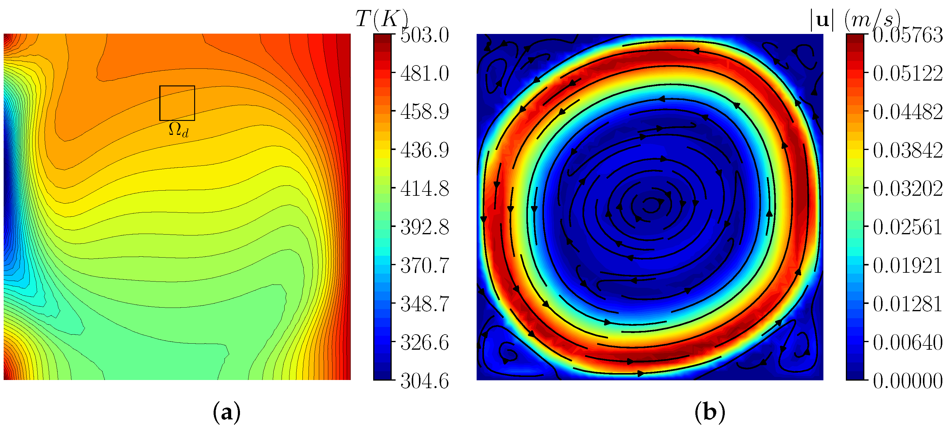
The contours of the optimal solution in terms of temperature and velocity fields are shown in Figure 3a,b, respectively, for $\lambda ={10}^{-7}$. The region ${\Omega }_d$, where the objective is set, is highlighted with a black square in Figure 3a. From the contours, we can see that the optimal temperature field assumes values close to the target temperature $T_d=450\mathrm{K}$. To achieve the objective, the temperature on the left wall decreases with respect to the reference case. For this reason, the motion changes, and we obtain a counterclockwise vortex, as depicted by the streamlines in Figure 3b.

In

Table 2. Temperature matching case with Dirichlet boundary control: objective functional, percentage reduction, and number of iterations of the optimization algorithm for different $\lambda$ values.

$\mathit{\lambda }$	${10}^{-5}$	${10}^{-6}$	${10}^{-7}$	${10}^{-8}$	Reference
${\mathcal{J}}^{\left(n\right)}\times {10}^6$	3.110	2.179	2.091	1.979	1250
% Reduction	$99.75$	$99.82$	$99.83$	$99.84$	0
Iterations n	6	5	6	10	0

, we report the objective functional values ${\mathcal{J}}^{\left(n\right)}$ corresponding to its optimal state for each numerical simulation. We also report the value of the reference objective functional ${\mathcal{J}}^{\left(0\right)}$ and the percentage reduction for each case evaluated as $({\mathcal{J}}^{\left(0\right)}-{\mathcal{J}}^{\left(n\right)})/{\mathcal{J}}^{\left(0\right)}$. In addition, the number of iterations n of the optimization algorithm is included in Table 2. The lowest value of $\lambda$ results in the lowest functional value of ${\mathcal{J}}^{\left(10\right)}=1.979\times {10}^{-6}$ and the greatest percentage reduction.

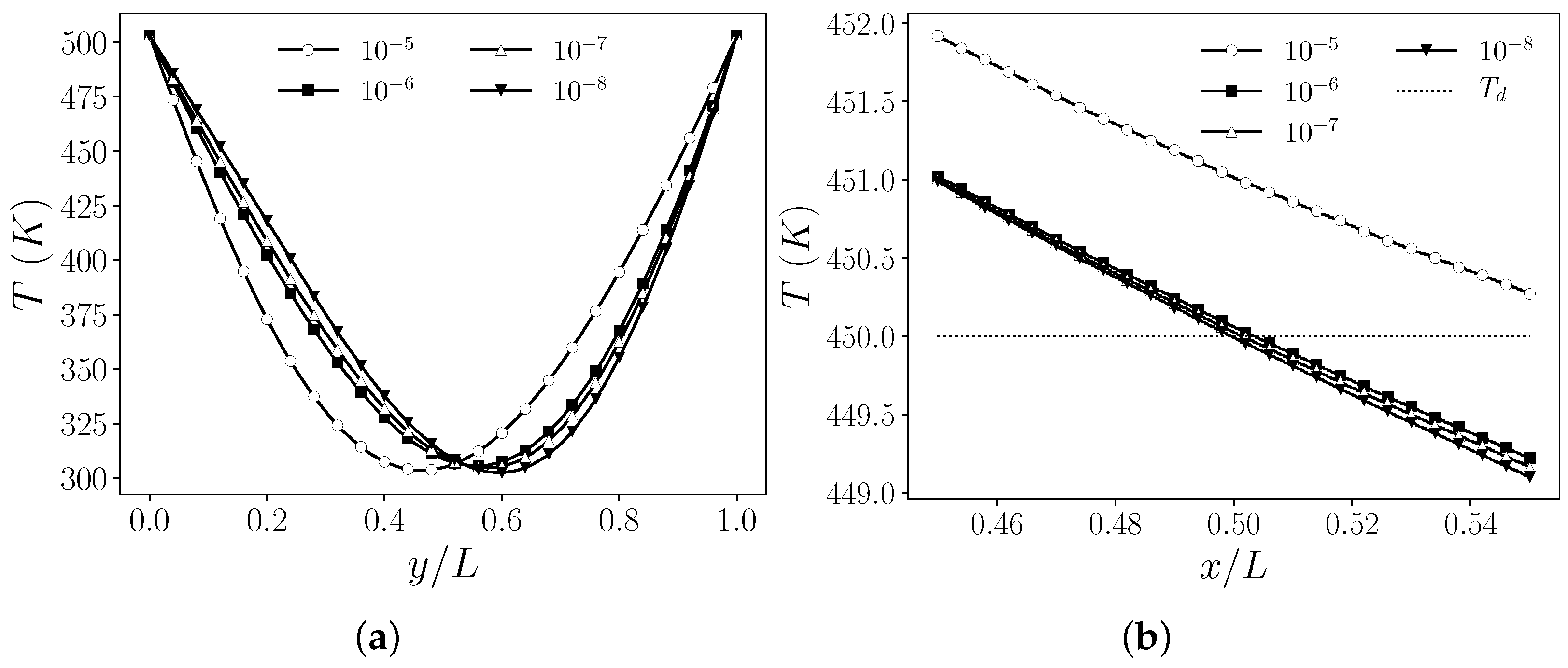
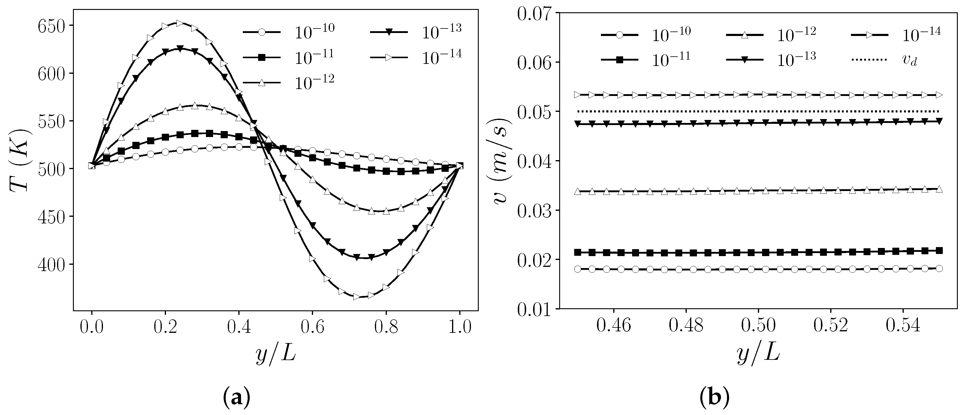
Temperature profiles along the boundary ${\Gamma }_c$ are reported in Figure 4a for the different values of the regularization parameter $\lambda$. As $\lambda$ decreases, the minima of the profiles move towards $y/L=1$. In Figure 4b, the temperature is plotted along a line at $y/L=0.8$ for $0.45<x/L<0.55$ in the region ${\Omega }_d$. We can see that for the lowest values of $\lambda$, the optimal solutions tend to the target profile $T_d$. The case $\lambda ={10}^{-5}$ is the farthest from the objective, as we can also deduce from the functional values reported in Table 2.

4.1.2. Velocity Matching Case 1

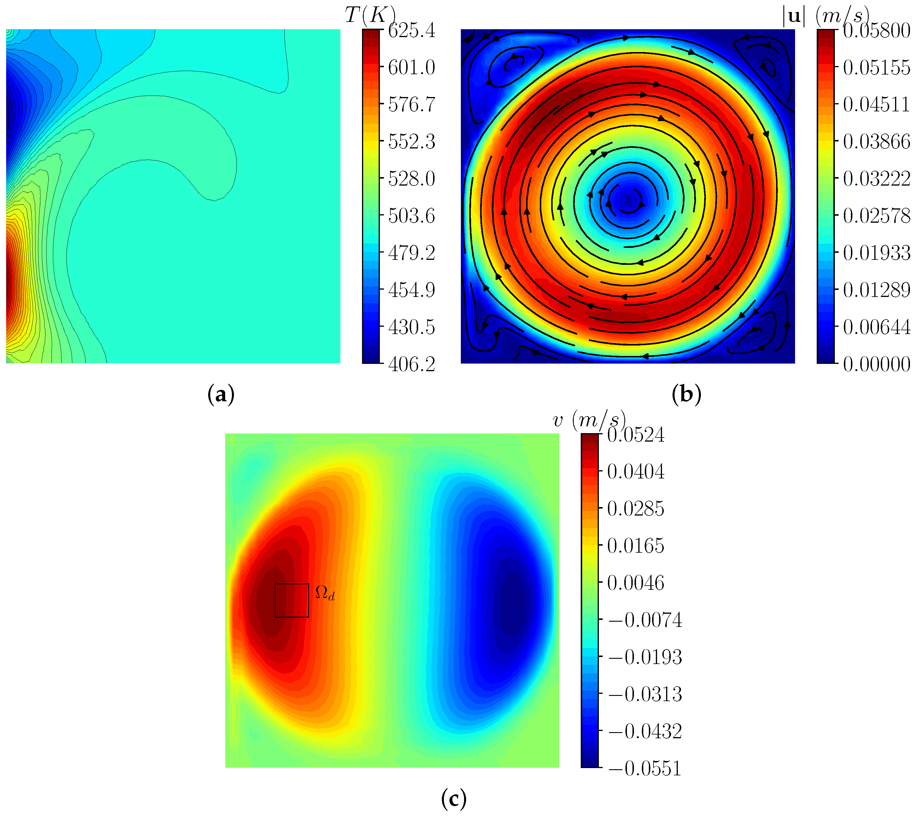
The second test for the Dirichlet optimal control is a velocity matching case. The objective functional is the one reported in Equation (13), setting ${\alpha }_u=1$, ${\alpha }_T=0$ and ${\Omega }_d=[0.15L;0.25L]\times [0.45L;0.55L]$. The region ${\Omega }_d$ is represented in Figure 5c. We aim to control the y-component of the velocity with $v_d=0.05\mathrm{m}/\mathrm{s}$. In the reference case, the mean value of v over ${\Omega }_d$ is $0.0159\mathrm{m}/\mathrm{s}$, but we aim to accelerate the fluid near the controlled boundary ${\Gamma }_c$ in order to enhance the velocity on ${\Omega }_d$. We consider different values of the regularization parameter $\lambda$, i.e., ${10}^{-10},{10}^{-11},{10}^{-12}$, ${10}^{-13}$, and ${10}^{-14}$. The considered values are lower than those used for the temperature matching test. We also tested higher values of the regularization parameter, but the control was ineffective in those cases. Indeed, it is easier to achieve an objective on the temperature field than on the velocity field, since the control parameter $T_c$ (or h or Q) depends directly on the adjoint temperature but indirectly on the adjoint velocity. The value of the reference objective functional is ${\mathcal{J}}^{\left(0\right)}=7.011\times {10}^{-10}$.

In Figure 5, the optimal solution obtained with $\lambda ={10}^{-13}$ is reported. In Figure 5a, the contours of the optimal temperature field are shown. Along ${\Gamma }_c$, the temperature shows a sharp variation. At the bottom of ${\Gamma }_c$, we have a maximum for the temperature, while at the top is the minimum temperature value. The fluid is heated and is accelerated to the desired velocity in the region ${\Omega }_d$. The resulting velocity field is shown in Figure 5b, where contours of the velocity magnitude and streamlines are shown. The contours of the y-component of the velocity are shown in Figure 5c, where the region ${\Omega }_d$ is highlighted.

In

Table 3. Velocity matching case with Dirichlet boundary control. Case 1: objective functional, percentage reduction, and number of iterations of the optimization algorithm for different $\lambda$ values.

$\mathit{\lambda }$	${10}^{-10}$	${10}^{-11}$	${10}^{-12}$	${10}^{-13}$	${10}^{-14}$	Reference
${\mathcal{J}}^{\left(n\right)}\times {10}^{12}$	586.3	413.6	137.4	9.767	8.796	701.1
% Reduction	$16.4$	$41.01$	$80.40$	$98.61$	$98.74$	0
Iterations n	5	5	4	6	5	0

, we report the objective functional values ${\mathcal{J}}^{\left(n\right)}$, the number of iterations n of the optimization algorithm, and the percentage reduction with respect to the reference ${\mathcal{J}}^{\left(0\right)}$. For the highest values of $\lambda$, the control is poor, and the functional is quite similar to the reference value. However, we can observe a strong functional reduction for the cases with $\lambda \le {10}^{-13}$.

Temperature profiles along the boundary ${\Gamma }_c$ are reported in Figure 6a for different values of the regularization parameter $\lambda$. For $\lambda ={10}^{-10}$, the profile only has a stationary point at $y/L\approx 0.5$. For lower values of $\lambda$, there is a change of concavity in the temperature profiles and an inflection point at $y/L\approx 0.5$. As $\lambda$ decreases, the maximum is located at $0.2<y/L<0.4$ and its value increases, while the minimum is located at $0.6<y/L<0.8$ and its value decreases. As expected, with low values of the regularization parameter, the $H^{-1}\left({\Gamma }_c\right)$-norm of the control has less weight in the objective functional, and more irregular functions are accepted as optimal solutions. In Figure 6b, the y-component of the velocity is plotted along a line at $x/L=0.2$ for $0.45<y/L<0.55$ in the region ${\Omega }_d$. The velocity profile is reported for all values of $\lambda$, together with the target velocity profile $v_d$. For the lowest values of $\lambda$ (${10}^{-13}$, ${10}^{-14}$), the optimal solutions tend to the target profile $v_d$, while the highest values of $\lambda$ (${10}^{-10},{10}^{-11}$, ${10}^{-12}$) lead to the solutions farthest from the objective, as can be deduced from the functional values in Table 3. However, when $\lambda$ is small (${10}^{-13}$, ${10}^{-14}$), the maximum temperature value increases (from $503\mathrm{K}$ up to $650\mathrm{K}$) and the minimum value decreases (from $503\mathrm{K}$ down to $400\mathrm{K}$). This large variation is due to the fact that the target $v_d$ is quite far from the reference case, and the temperature over ${\Gamma }_c$ must change considerably to reach the objective.

4.1.3. Velocity Matching Case 2

A second case for the velocity matching test is now considered. The objective is set on the x-component of the velocity field, where we aim to achieve a counterclockwise flow. Let us consider ${\Omega }_d=[0.45L;0.55L]\times [0.75L;0.85L]$. This region is highlighted in Figure 7c. In the reference case, the mean value of u on ${\Omega }_d$ is set to $0.0129\mathrm{m}/\mathrm{s}$. Then, we set a uniform value $u_d=-0.02\mathrm{m}/\mathrm{s}$ as a target profile. The simulations are performed considering different values of $\lambda$, namely, ${10}^{-10},{10}^{-11}$, and ${10}^{-12}$. The reference objective functional is ${\mathcal{J}}^{\left(0\right)}=5.425\times {10}^{-10}$.

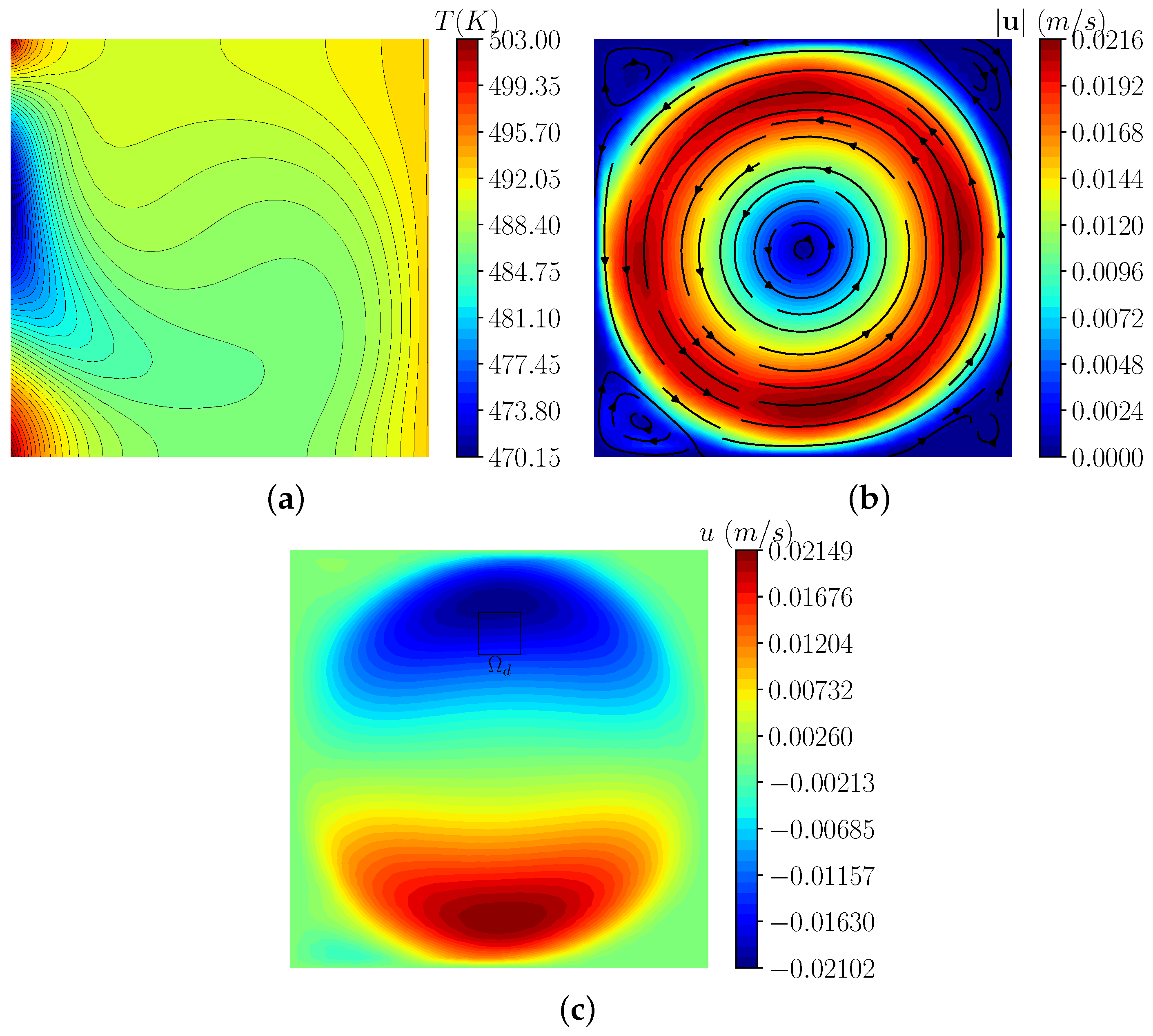
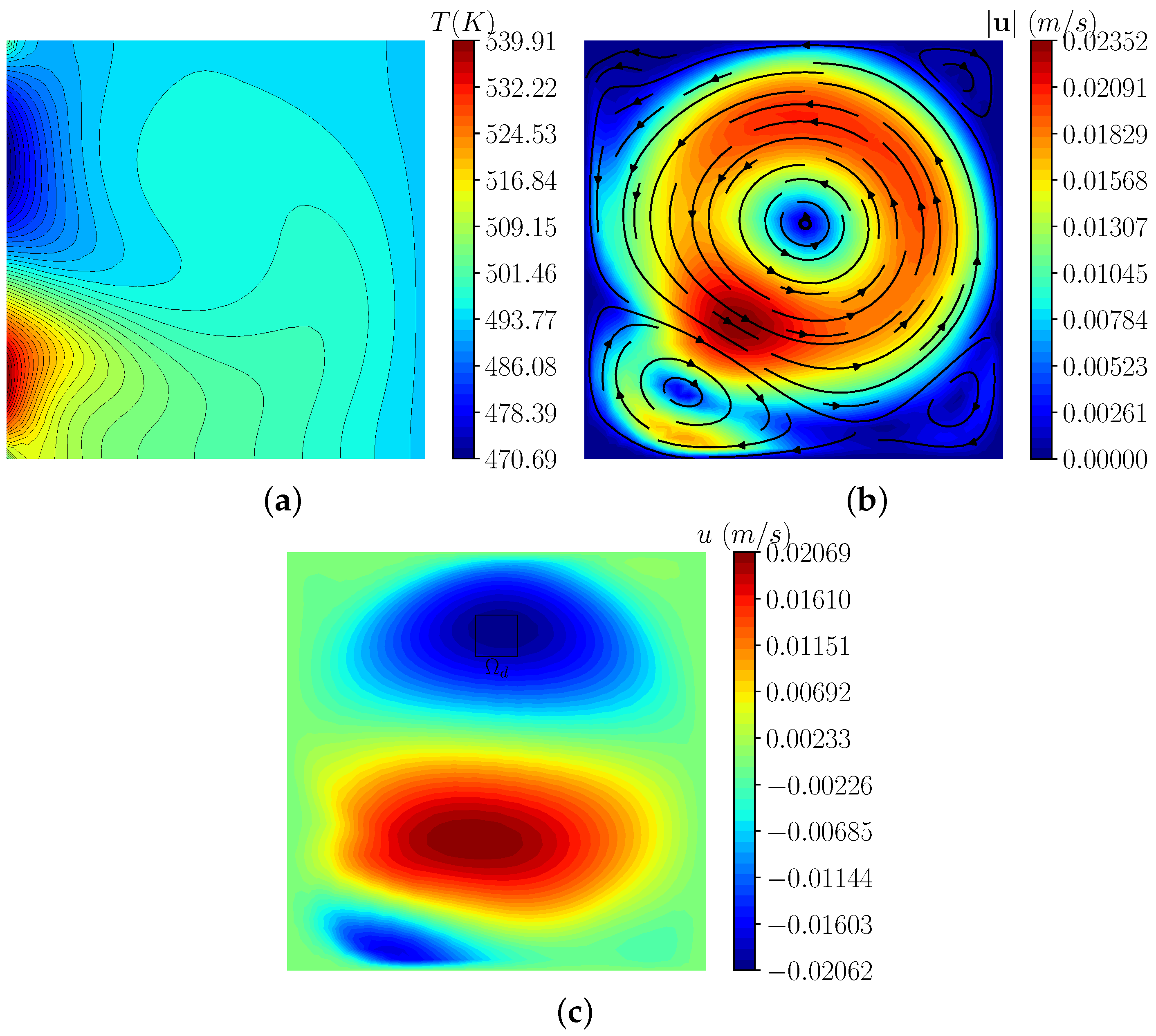
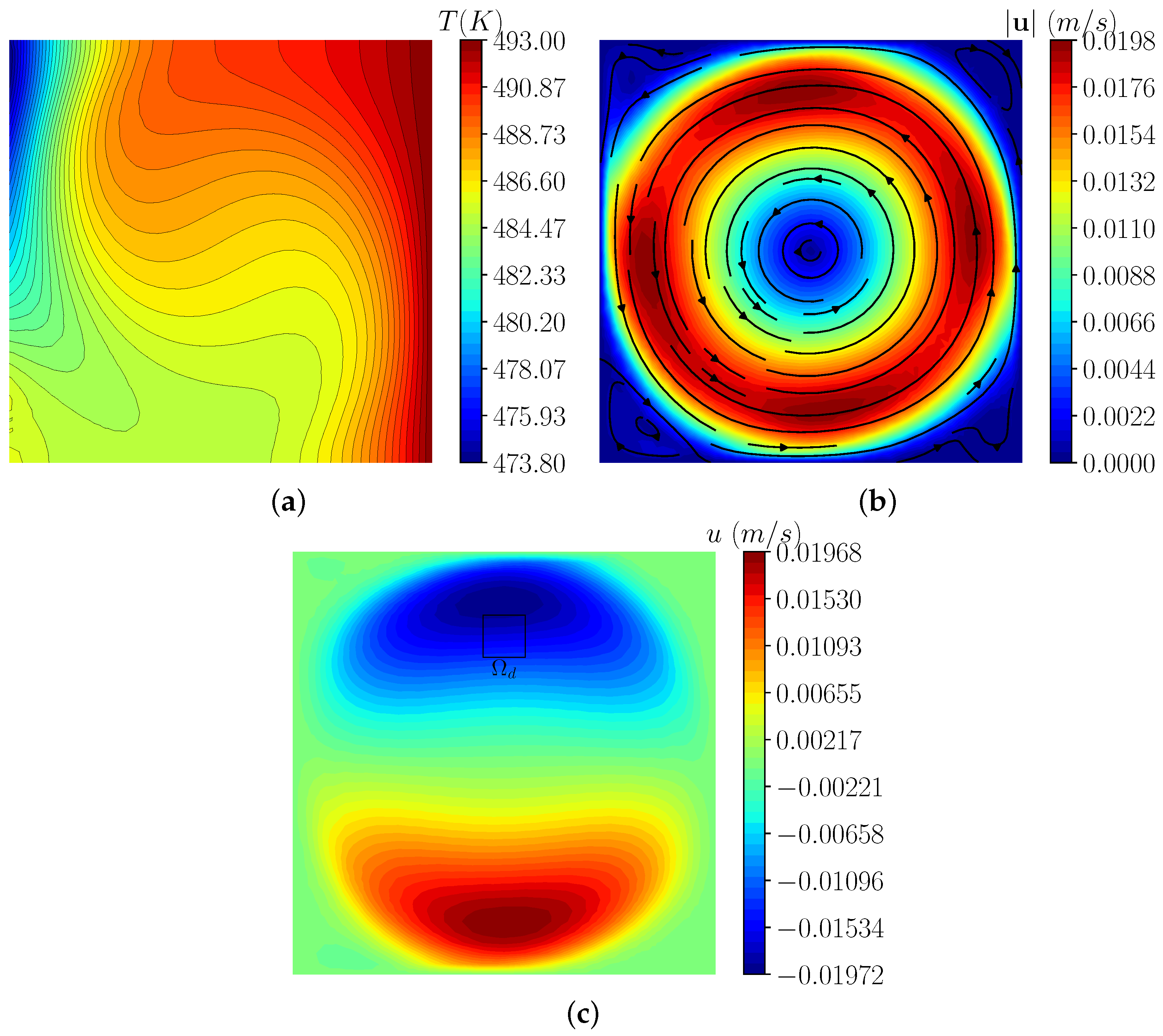
The optimal temperature and velocity fields obtained with $\lambda ={10}^{-11}$ are reported in Figure 7. In Figure 7a, the contours of the optimal temperature field are shown. The resulting velocity field is shown in Figure 7b, where contours of the velocity magnitude and streamlines are reported. We can observe that a counterclockwise flow is driven by the buoyancy forces. The contours of the x-component of the velocity are represented in Figure 7c, where the region ${\Omega }_d$ is highlighted. We also report the optimal solution obtained with $\lambda ={10}^{-12}$ in Figure 8. In this case, the solution is quite unexpected. Figure 8a shows the contours of the optimal temperature field. At the bottom of the left wall (${\Gamma }_c={\Gamma }_1$), the temperature is higher than the temperature on the right wall (${\Gamma }_i={\Gamma }_3$), while at the top of ${\Gamma }_c$ the temperature is lower than the temperature on ${\Gamma }_3$.

This profile induces buoyancy forces which cause two vortexes; a smaller clockwise vortex behind the bottom-left corner and a bigger counterclockwise vortex in the center of the cavity, as shown in Figure 8b. The contours of the x-component of velocity are shown in Figure 8c, where the region ${\Omega }_d$ is in evidence. There, the x-component of velocity is quite uniform and close to the target value $u_d$.

In

Table 4. Velocity matching case with Dirichlet boundary control—Case 2: objective functional, percentage reduction and number of iterations of the optimization algorithm for different $\lambda$ values.

$\mathit{\lambda }$	${10}^{-10}$	${10}^{-11}$	${10}^{-12}$	Reference
${\mathcal{J}}^{\left(n\right)}\times {10}^{13}$	246.6	36.04	1.677	5423
% Reduction	$54.53$	$93.35$	$99.69$	0
Iterations n	4	10	9	0

, we report the objective functional values ${\mathcal{J}}^{\left(n\right)}$, the percentage reduction, and the number of iterations n of the optimization algorithm. For the highest value of $\lambda$ (${10}^{-10}$), the control is poor, and the functional value is quite similar to the reference value. For the other values of $\lambda$, the control is more effective. As observed in the previous test cases, with the lowest value of $\lambda$, we have the lowest functional value and the greatest percentage reduction.

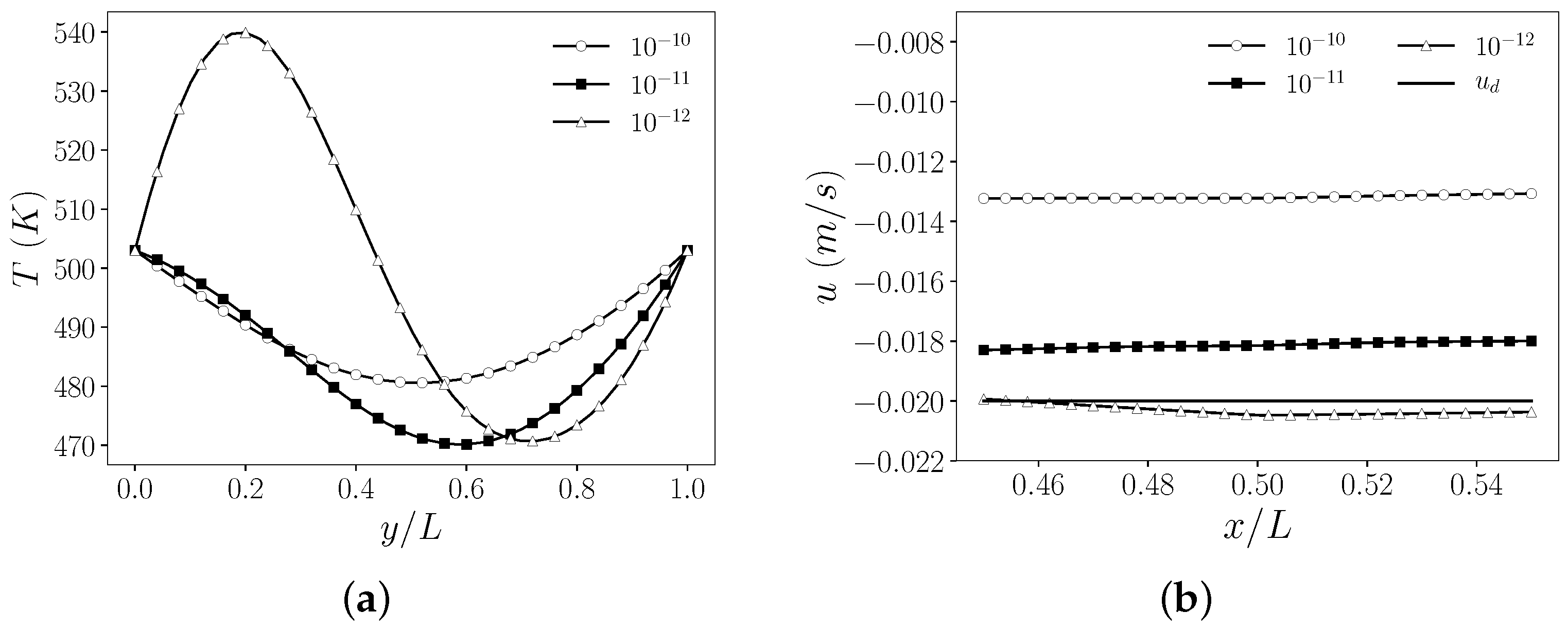
In Figure 9a, the temperature profiles along the boundary ${\Gamma }_c$ are shown for different values of the regularization parameter $\lambda$ (${10}^{-10}$, ${10}^{-11}$, ${10}^{-12}$). For $\lambda ={10}^{-10}$ and $\lambda ={10}^{-11}$, the profiles present a minimum point at $0.4<y/L<0.7$. The temperature on ${\Gamma }_c$ is lower than the temperature on the opposite wall ${\Gamma }_i$, namely, $T=493\mathrm{K}$, to obtain a counterclockwise flow. For $\lambda ={10}^{-12}$, the optimal solution is unexpected, as previously noted. There is a variation of concavity in the profile and an inflection point at $y/L\approx 0.5$. For $y/L<0.5$, the temperature on ${\Gamma }_c$ is higher than the temperature on ${\Gamma }_3$, while at the top of the controlled wall, for $y/L>0.5$, the temperature on ${\Gamma }_c$ is lower than the temperature on ${\Gamma }_3$. In Figure 9b, the x-component of the velocity is plotted along a line at $y/L=0.8$ for $0.45<x/L<0.55$ in the region ${\Omega }_d$. The velocity profiles are shown for all values of $\lambda$, together with the target velocity profile $u_d$. We can observe that in all cases, the flow changes from clockwise to counterclockwise with a negative x-component of velocity at the top of the cavity. We note that in this test, the lower the value of $\lambda$, the closer the velocity profile is to the target profile.

4.2. Neumann Boundary Control

For the Neumann control problem, we consider the geometry shown in Figure 1. The boundary conditions are reported in (38), where ${\Gamma }_d={\Gamma }_3$, ${\Gamma }_n={\Gamma }_1\cup {\Gamma }_2\cup {\Gamma }_4$, ${\Gamma }_i={\Gamma }_2\cup {\Gamma }_4$, ${\Gamma }_c={\Gamma }_1$. We set $g_{t,n}=0$, $g_t=493\mathrm{K}$, and ${\mathbf{g}}_u=\mathbf{0}$ in (38) and $\mathbf{f}=\mathbf{0}$, $Q=0$ in (40). The wall-normal heat flux h acting on ${\Gamma }_c$ is the control for the problem. To compute the reference case, we set $h^{\left(0\right)}=0$. Thus, the uncontrolled problem consists of three thermally-insulated walls, i.e., the left (${\Gamma }_1$), bottom (${\Gamma }_2$), and top (${\Gamma }_4$) walls, and a wall with a fixed temperature, which is the right wall (${\Gamma }_3$). The reference case is a trivial problem, characterized by a uniform and constant temperature, no buoyancy forces, and still fluid.

We performed several tests, varying the objective. We report the numerical results obtained considering the same objective on the x-component of velocity also studied with the Dirichlet control. We recall the main simulation parameters. Let ${\Omega }_d=[0.45L;0.55L]\times [0.75L;0.85L]$ be the region where we aim to achieve the objective, and let $u_d=-0.02\mathrm{m}/\mathrm{s}$ be the target velocity profile. In the reference case, the fluid is still. Then, $u=0\mathrm{m}/\mathrm{s}$ in ${\Omega }_d$. The simulations were performed considering different values of $\lambda$, namely, ${10}^{-4}$, ${10}^{-5},{10}^{-6}$, and ${10}^{-7}$. The reference objective functional is ${\mathcal{J}}^{\left(0\right)}=2.061\times {10}^{-10}$.

In

Table 5. Velocity matching case with Neumann boundary control: objective functional, percentage of reduction, and number of iterations of the optimization algorithm for the reference case and different $\lambda$ values.

$\mathit{\lambda }$	${10}^{-4}$	${10}^{-5}$	${10}^{-6}$	${10}^{-7}$	Reference
${\mathcal{J}}^{\left(n\right)}\times {10}^{12}$	30.58	30.14	8.454	1.536	206.1
% Reduction	$85.16$	$85.8$	$95.90$	$99.25$	0
Iterations n	4	14	9	7	0

, the objective functional values ${\mathcal{J}}^{\left(n\right)}$ and the number of iterations n of the optimization algorithm are reported for all the values of $\lambda$. The percentage reductions are also reported. In all tests, we observe large functional reductions. In particular, for lower values of $\lambda$, the control is more effective.

The optimal solution obtained with $\lambda ={10}^{-6}$ is reported in Figure 10. The contours of the temperature field T over the domain can be seen in Figure 10a. The heat flux imposed on the left wall is outgoing, and the wall is cooler than in the reference case, with a minimum value of around 473 K. In Figure 10b, the velocity streamlines and the contours of the velocity magnitude are shown. The formation of a counterclockwise vortex is shown in this figure. The contours of the x-component of the velocity field u are reported in Figure 10, and the region ${\Omega }_d$ is highlighted.

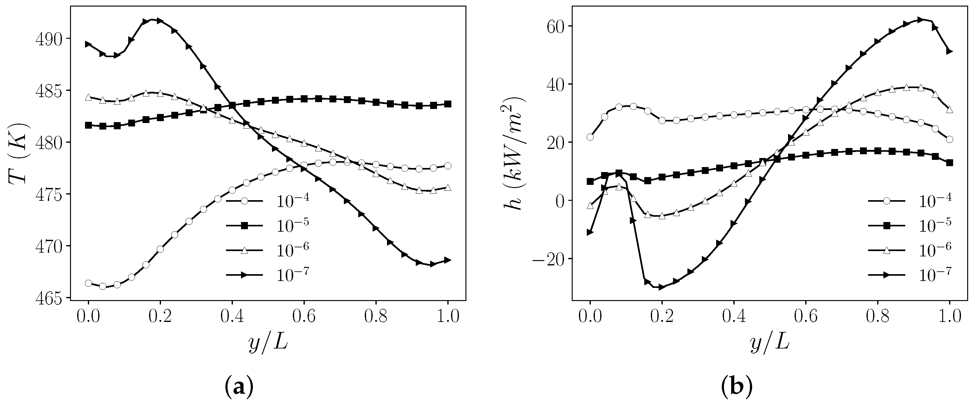
In Figure 11a, the temperature profiles along the boundary ${\Gamma }_c$ are shown for different values of the regularization parameter $\lambda$ (${10}^{-4}$, ${10}^{-5}$, ${10}^{-6}$, ${10}^{-7}$). Comparing these profiles with the temperature profiles of Figure 9a obtained for a Dirichlet control, we observe very different trends. With a Dirichlet control, the temperature on ${\Gamma }_c$ belongs to the Hilbert space $H^1\left({\Gamma }_c\right)$, and the control $T_c$ is nullified at the extremities of the boundary, i.e., $T_c=0\mathrm{K}$ on $\partial {\Gamma }_c$. For this reason, with a Dirichlet control, $T=g_t=503\mathrm{K}$ at $y/L=0$ and $y/L=1$. With Neumann controls, we do not have constraints on the temperature value on $\partial {\Gamma }_c$, and we obtain different shapes for the profiles. In Figure 11b, the control parameter h expressed in ${\mathrm{kW}/\mathrm{m}}^2$ is reported along ${\Gamma }_c$. With the highest values of $\lambda$ (${10}^{-4}$, ${10}^{-5}$), the control is quite uniform and regular, but it is less effective with respect to the functional reduction. With the lowest values of $\lambda$ (${10}^{-6}$, ${10}^{-7}$), the profiles of the control h are sharp and present changes of sign.

4.3. Distributed Control

For the distributed control problem, we consider the geometry reported in Figure 1. The boundary conditions are reported in (9), where ${\Gamma }_d={\Gamma }_1\cup {\Gamma }_3$, ${\Gamma }_n={\Gamma }_2\cup {\Gamma }_4$. We set $\mathbf{f}=0$, ${\mathbf{g}}_u=0$ in (62), while in (9) we have $g_{t,n}=0$, $g_t=493\mathrm{K}$ on ${\Gamma }_3$, and $g_t=503\mathrm{K}$ on ${\Gamma }_1$. The volumetric heat source Q is the control acting on the domain $\Omega$. For the reference case, we consider $Q^{\left(0\right)}=0$. Thus, the reference case is the one considered for the Dirichlet boundary control. The buoyancy forces put the fluid in motion, and a clockwise vortex is formed. The contours and streamlines for the temperature and velocity are shown in Figure 2.

We performed several tests, varying the objectives and the values of the regularization parameter $\lambda$. We show the results for a velocity matching case. Let us consider ${\Omega }_d=[0.15L;0.25L]\times [0.45L;0.55L]$. We aim to control the y-component of the velocity, and therefore we set $v_d=0.05\mathrm{m}/\mathrm{s}$, as in the first velocity matching case presented for the Dirichlet boundary control. In the reference case, the mean value of v on ${\Omega }_d$ is equal to $0.0159\mathrm{m}/\mathrm{s}$, as we aim to accelerate the fluid near the controlled boundary ${\Gamma }_c$. We consider several values of the regularization coefficient, namely, ${10}^{-10}$, ${10}^{-11}$, and ${10}^{-12}$.

In

Table 6. Velocity matching case with distributed control: objective functional ${\mathcal{J}}^{\left(n\right)}$, percentage reduction, and number of iterations n of the optimization algorithm for different values of $\lambda$.

$\mathit{\lambda }$	${10}^{-10}$	${10}^{-11}$	${10}^{-12}$	Reference
${\mathcal{J}}^{\left(n\right)}\times {10}^{13}$	2.792	2.229	2.159	2061
% Reduction	$99.96$	$99.97$	$99.97$	0
Iterations n	3	13	35	0

, the objective functional values ${\mathcal{J}}^{\left(n\right)}$, the percentage reductions, and the number of iterations n of the optimization algorithm are reported for all values of $\lambda$. Thus, in all the tests, the functional is strongly reduced by a factor of ${10}^3$. This is an expected result since the optimal control Q can act on the whole domain, and its influence is strong on the distribution of the temperature field and buoyancy forces. We remark that with boundary control problems, the control can act only on a portion of the boundary, and its impact is less effective on the solution.

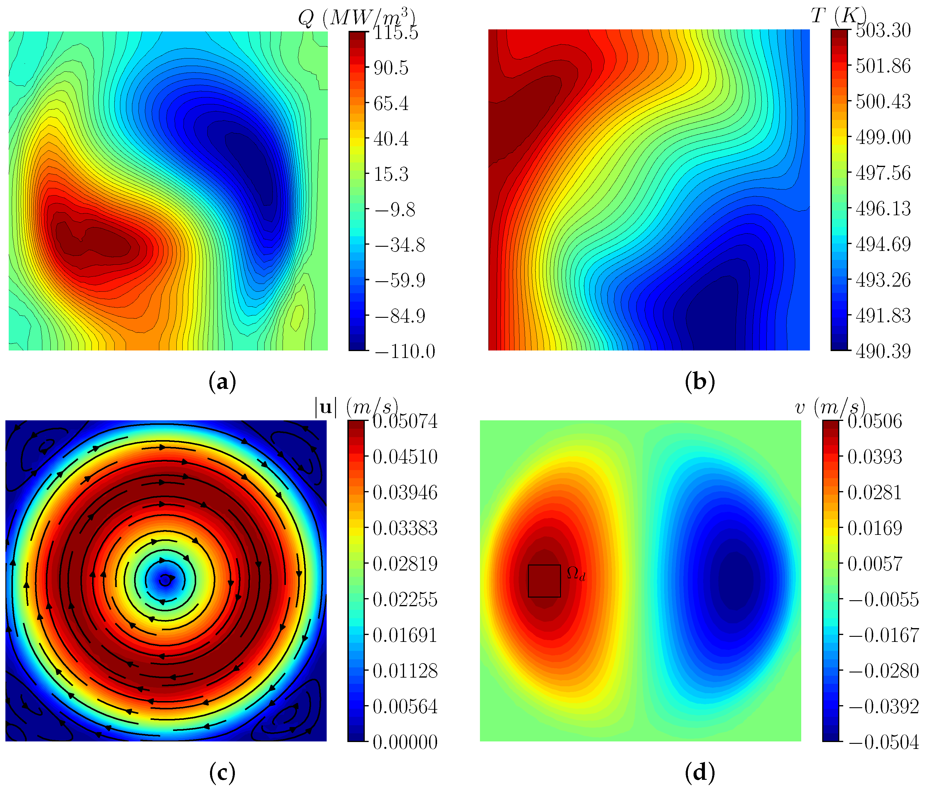
In Figure 12, the contours of the optimal solution for $\lambda ={10}^{-11}$ are shown. The optimal control Q expressed in ${\mathrm{MW}/\mathrm{m}}^3$ is reported in Figure 12a. The heat source is not uniform over the domain, being positive in the proximity of the hottest wall ($T=503\mathrm{K}$ on ${\Gamma }_1$) and negative near the coolest wall ($T=493\mathrm{K}$ on ${\Gamma }_3$). This heat source distribution influences the temperature solution reported in Figure 12b. The isotherms are more stretched than in the reference case, and the fluid is locally hotter than $503\mathrm{K}$ and cooler than $493\mathrm{K}$, due to the volumetric heat source. The streamlines and contours of the velocity field are reported in Figure 12c. Figure 12d shows the region ${\Omega }_d$ and the contours of the y-component of velocity. The solution is almost uniform in ${\Omega }_d$ and is close to the target value of $v_d=0.02\mathrm{m}/\mathrm{s}$. Comparing Figure 5c and Figure 12d, we can observe that the distributed control is the most effective in achieving the objective. The great effectiveness of the distributed control can be also seen by comparing Table 6 and the first three columns of Table 3. With the same $\lambda$ coefficients (${10}^{-10}$, ${10}^{-11}$, and ${10}^{-12}$), the distributed control leads to much greater reductions in the functional ${\mathcal{J}}^{\left(n\right)}$ than the Dirichlet control. Moreover, by observing Figure 5a and Figure 12b, we see that with a distributed control, the optimal temperature solution is more uniform and regular than with a Dirichlet optimal control, which can lead to temperature variations that may not be acceptable in a practical context.

5. Conclusions

In this work, optimal control problems for incompressible Newtonian buoyant flows were presented and discussed. Starting from some important results already presented in previous studies on the existence of an optimal solution and the existence of the Lagrange multipliers, we analyzed Dirichlet, Neumann, and distributed optimal control problems. For each case, we obtained the optimality system, which consists of state, adjoint, and control equations. To solve this numerically, a gradient method was introduced, and an efficient numerical algorithm was proposed for each case. We observed that the three control mechanisms differed only in the control equation, which is an algebraic equation in the case of distributed and Neumann control and a differential equation in the case of Dirichlet control. In all the mechanisms, the controls depended on the adjoint temperature field $T_a$ and on the regularization parameter $\lambda$. Numerical simulations were performed to test the robustness of the algorithm and the feasibility of the method. The developed numerical simulations included velocity matching cases and temperature matching cases, both evaluated with various values of the regularization parameter $\lambda$. We observed that the temperature matching case is easier to achieve, since in this case the distance from the target temperature appears directly as source term in the adjoint temperature equation. The choice of the value of the regularization parameters proved to be a key issue: too much regularization leads to smoother but less effective controls, while a lack of regularization causes numerical issues and singular solutions. We observed that the appropriate choice of $\lambda$ should be made on a case-by-case basis. A comparison among the three thermal control mechanisms allowed us to draw some conclusions as follows. The strongest control is the distributed control, followed by the Neumann and Dirichlet boundary controls. Of course, all these three different controls can be feasible at different costs, depending on the engineering applications. In general, the developed numerical algorithm showed good convergence properties and thus can be considered a useful tool for the numerical resolution of optimal control problems for Boussinesq equations.

References

- Chirco, L.; Chierici, A.; Da Vià, R.; Giovacchini, V.; Manservisi, S. Optimal Control of the Wilcox turbulence model with lifting functions for flow injection and boundary control. J. Phys. Conf. Ser. 2019, 1224, 012006. [Google Scholar] [CrossRef]
- Gunzburger, M.D.; Hou, L.S.; Svobodny, T.P. The approximation of boundary control problems for fluid flows with an application to control by heating and cooling. Comput. Fluids 1993, 22, 239–251. [Google Scholar] [CrossRef]
- Lee, H.C. Analysis and computational methods of Dirichlet boundary optimal control problems for 2D Boussinesq equations. Adv. Comput. Math. 2003, 19, 255–275. [Google Scholar] [CrossRef]
- Aulisa, E.; Bornia, G.; Manservisi, S. Boundary control problems in convective heat transfer with lifting function approach and multigrid vanka-type solvers. Commun. Comput. Phys. 2015, 18, 621–649. [Google Scholar] [CrossRef]
- Lee, H.C.; Shin, B.C. Piecewise optimal distributed controls for 2D Boussinesq equations. Math. Methods Appl. Sci. 2000, 23, 227–254. [Google Scholar] [CrossRef]
- Gunzburger, M.D.; Kim, H.; Manservisi, S. On a shape control problem for the stationary Navier-Stokes equations. ESAIM Math. Model. Numer. Anal. 2000, 34, 1233–1258. [Google Scholar] [CrossRef] [Green Version]
- Gunzburger, M.D. Perspectives in Flow Control and Optimization; SIAM: Philadelphia, PA, USA, 2003; Volume 5. [Google Scholar]
- Smith, C.F.; Cinotti, L. Lead-cooled fast reactor. In Handbook of Generation IV Nuclear Reactors; Elsevier: Amsterdam, The Netherlands, 2016; pp. 119–155. [Google Scholar]
- Lee, H.C.; Imanuvilov, O.Y. Analysis of optimal control problems for the 2-D stationary Boussinesq equations. J. Math. Anal. Appl. 2000, 242, 191–211. [Google Scholar] [CrossRef] [Green Version]
- Lee, H.C. Optimal control problems for the two dimensional Rayleigh—Bénard type convection by a gradient method. Jpn. J. Ind. Appl. Math. 2009, 26, 93–121. [Google Scholar] [CrossRef]
- Lee, H.C.; Kim, S.H. Finite element approximation and computations of optimal Dirichlet boundary control problems for the Boussinesq equations. J. Korean Math. Soc. 2004, 41, 681–715. [Google Scholar] [CrossRef] [Green Version]
- Lee, H.C. Analysis and computations of Neumann boundary optimal control problems for the stationary Boussinesq equations. In Proceedings of the 40th IEEE Conference on Decision and Control (Cat. No. 01CH37228), Orlando, FL, USA, 4–7 December 2001; Volume 5, pp. 4503–4508. [Google Scholar]
- Alekseev, G. Solvability of stationary boundary control problems for heat convection equations. Sib. Math. J. 1998, 39, 844–858. [Google Scholar] [CrossRef]
- Alekseev, G.; Tereshko, D. Boundary control problems for stationary equations of heat convection. In New Directions in Mathematical Fluid Mechanics; Springer: Berlin/Heidelberg, Germany, 2009; pp. 1–21. [Google Scholar]
- Baranovskii, E.S.; Domnich, A.A.; Artemov, M.A. Optimal boundary control of non-isothermal viscous fluid flow. Fluids 2019, 4, 133. [Google Scholar] [CrossRef] [Green Version]
- Baranovskii, E.S. Optimal boundary control of the Boussinesq approximation for polymeric fluids. J. Optim. Theory Appl. 2021, 189, 623–645. [Google Scholar] [CrossRef]
- Baranovskii, E.S. The optimal start control problem for two-dimensional Boussinesq equations. Izv. Math. 2022, 86, 221–242. [Google Scholar] [CrossRef]
- Ciarlet, P.G. The Finite Element Method for Elliptic Problems; SIAM: Philadelphia, PA, USA, 2002. [Google Scholar]
- Droniou, J. Non-coercive linear elliptic problems. Potential Anal. 2002, 17, 181–203. [Google Scholar] [CrossRef]
- Chierici, A.; Giovacchini, V.; Manservisi, S. Analysis and numerical results for boundary optimal control problems applied to turbulent buoyant flows. Int. J. Numer. Anal. Model. 2022, 19, 347–368. [Google Scholar]
- Giovacchini, V. Development of a numerical platform for the modeling and optimal control of liquid metal flows. Ph.D. Thesis, University of Bologna, Bologna, Italy, 2022. [Google Scholar]
- Chierici, A.; Barbi, G.; Bornia, G.; Cerroni, D.; Chirco, L.; Da Vià, R.; Giovacchini, V.; Manservisi, S.; Scardovelli, R.; Cervone, A. FEMuS-Platform: A numerical platform for multiscale and multiphysics code coupling. In Proceedings of the 9th edition of the International Conference on Computational Methods for Coupled Problems in Science and Engineering (COUPLED PROBLEMS 2021), Virtual, 13–16 June 2021. [Google Scholar]
- Barakos, G.; Mitsoulis, E.; Assimacopoulos, D. Natural convection flow in a square cavity revisited: Laminar and turbulent models with wall functions. Int. J. Numer. Methods Fluids 1994, 18, 695–719. [Google Scholar] [CrossRef]
Figure 1.
Computational domain for the optimal control of Boussinesq equations, where is the gravity vector and , , , and are the boundaries.
Figure 2.
Uncontrolled solution: contours of the temperature field T (a); contours and streamlines of the velocity field (b). The velocity magnitude is indicated by .
Figure 3.
Temperature matching case with Dirichlet boundary control: optimal solution for . Contours of the temperature field T (a); contours and streamlines of the velocity field (b). The velocity magnitude is indicated by , and is the region where the objective is set.
Figure 4.
Temperature matching case with Dirichlet boundary control: temperature T profiles plotted against along the controlled boundary (a); temperature T profiles plotted against on the region along the line (b). Numerical results for , and . The target value is shown as a dotted line.
Figure 5.
Velocity matching case with Dirichlet boundary control—Case 1: optimal solution for . Contours of the temperature field T (a); contours and streamlines of the velocity field (b); contours of the y-component of the velocity field v (c). The velocity magnitude is indicated by , and is the region where the objective is set.
Figure 6.
Velocity matching case with Dirichlet boundary control—Case 1: temperature profiles T plotted against on the controlled boundary (a); y-component of the velocity v profiles plotted against on the region along the line (b). Numerical results for , and . The target value is shown as a dotted line.
Figure 7.
Velocity matching case with Dirichlet boundary control—Case 2: optimal solution for . Contours of the temperature field T (a); contours and streamlines of the velocity field (b); contours of the x-component of the velocity field u (c). The velocity magnitude is indicated by , and is the region where the objective is set.
Figure 8.
Figure 9.
Velocity matching case with Dirichlet boundary control—Case 2: temperature profiles T plotted against on the controlled boundary (a); x-component of the velocity u profiles plotted against on the region along the line (b). Numerical results for , and . The target value is shown as a dotted line.
Figure 10.
Velocity matching case with Neumann boundary control: optimal solution for . Contours of the temperature field T (a); contours and streamlines of the velocity field (b); contours of the x-component of the velocity field u (c). The velocity magnitude is indicated by , and is the region where the objective is set.
Figure 11.
Velocity matching case with Neumann boundary control: temperature T (a) and wall-normal heat flux h (b) plotted against on the controlled boundary . Numerical results for , and .
Figure 12.
Velocity matching case with distributed control: optimal solution for . Contours of the control Q (a); contours of the temperature field T (b); contours and streamlines of the velocity field (c); contours of the y-component of velocity v (d). The velocity magnitude is indicated by , and is the region where the objective is set.