
Two Models for 2D Deep Water Waves


1
Department of Physics, Novosibirsk State University, 630090 Novosibirsk, Russia
2
Skolkovo Institute of Science and Technology, 121205 Moscow, Russia
3
Landau Institute for Theoretical Physics, 142432 Chernogolovka, Russia
*
Authors to whom correspondence should be addressed.
Fluids 2022, 7(6), 204; https://0-doi-org.brum.beds.ac.uk/10.3390/fluids7060204
Submission received: 29 April 2022
/
Revised: 6 June 2022
/
Accepted: 9 June 2022
/
Published: 15 June 2022
(This article belongs to the Special Issue Nonlinear Wave Hydrodynamics, Volume II)
Abstract
:In this paper we propose two Hamiltonian models to describe two-dimensional deep water waves propagating on the surface of an ideal incompressible three-dimensional fluid. The idea is based on taking advantage of the Zakharov equation for one-dimensional waves which can be written in the form of so-called compact equations. We generalize these equations to the case of two-dimensional waves. As a test of our models, we perform numerical simulations of the dynamics of standing waves in a channel with smooth vertical walls. The results obtained in the proposed models are comparable, indicating that the models are similar to the original Zakharov equation.
1. Introduction
Physical phenomena related to deep water waves, for instance, the overturning of waves or the formation of so-called rogue waves, raise many questions for researchers. It is impossible to list all the efforts devoted to studying this field. In the general case, the dynamics of deep water waves propagating on the free surface can be described by the Laplace equation with nonlinear kinematic and dynamic boundary conditions at the surface. Solving these equations is a non-trivial task. Therefore, researchers use various simplified models.
At present, in the context of studying the dynamics of one-dimensional deep water waves, the only approximate model that is integrable in terms of the inverse scattering problem [1] is the well-known nonlinear Schrödinger equation (NLSE) [2]. Unfortunately, despite numerous advantages the model contains significant limitations that do not allow one to adequately describe the mentioned physical processes. Among the more accurate models one can highlight the Zakharov Equation [3]. Like the NLSE, it is based on perturbation theory where the small parameter is the wave steepness. It should be noticed that in the one-dimensional case the Zakharov equation can be rewritten in compact forms [4,5]. Another widely used method for solving the original equations, which is based on the expansion of velocity potential, is a high-order spectral method (HOSM) [6]. Finally, there is an exact model for describing the dynamics of one-dimensional deep water waves, a system of nonlinear equations written in conformal variables [7,8].
The problem becomes more complicated when considering two-dimensional waves propagating on the surface of a three-dimensional fluid. Exact equations in conformal variables can no longer be used in such geometry. Nevertheless, these equations with weak three-dimensional effects were considered in [9], and their corresponding numerical simulations were given in [10,11,12]. One straightforward variant is to use some two-dimensional version of the NLSE [13,14], but it is still very limited in its applicability [15]. Moreover, it is no longer an integrable model. A more accurate modification of the NLSE softening its limitations is in [16]. Intermediate model between the NLSE and the Zakharov equation can be found in [17]. Several studies on the physical phenomena and statistical properties of two-dimensional deep water waves using HOSM can be found in [18,19]. The Zakharov equation can also be used in the case of two-dimensional waves. However, there is considerable difficulty here that makes working with it quite challenging. The original Zakharov equation has a complex form that cannot be written in the way of some “compact” equations, as it was done in the one-dimensional case. Nevertheless, this equation is used to derive kinetic equations, in the manner of the Hasselmann equation [20], that allows studying weak turbulence in wind-driven sea [21,22].
This paper proposes two approximate Hamiltonian models to describe two-dimensional deep water waves propagating on the surface of a three-dimensional ideal incompressible fluid in a gravity field. The idea is based on using the advantages of the one-dimensional Zakharov equation. As mentioned earlier in this case it can be written in simple form of so-called compact equations. Then, these equations can be generalized to the case of two-dimensional waves. To verify the models for adequacy in describing deep water waves, we consider the dynamics of standing waves in a channel with smooth vertical walls.
The article is presented in the following way: the theoretical part, including the derivation of the proposed models from the Zakharov equation and their detailed description, will be shown in Section 2. Then, in Section 3, we present a description of the methods used in numerical simulations and the results obtained within the framework of the derived models. Finally, Section 4 will be devoted to a discussion of the results.
2. Hamiltonian Formalism for Deep Water Waves
Since the starting point for the proposed models is the Zakharov equation, we consider it necessary to briefly recall its derivation.
The 3D potential flow of an ideal incompressible deep fluid in the presence of a gravity field can be described by the following equations:
Here, the , z axis is directed away from the undisturbed surface coinciding with xy plane, t is time, g is the free-fall acceleration, is the shape of the surface, is the hydrodynamic potential inside the fluid, and is the potential at the surface.
The system is Hamiltonian and , is Hamiltonian variables [3]:
The expansion of the Hamiltonian in power series of and up to the fourth-order is as follows:
Here, operator means multiplication by in k space.
Applying canonical transformation (also see [3] for details) from and to the variables of b and , one can remove all non-resonant terms and drastically simplify the Hamiltonian:
Here, . The equation of motion in this case is a traditional Zakharov equation:
Here represents the coefficient of four-wave interactions. Despite the explicit expression [23], it does not allow writing the Zakharov equation in x space. Direct use of Equation (5) to describe the evolution of two-dimensional waves is quite challenging because it requires the calculation of four-dimensional integrals over . Applying a canonical transformation that would simplify the original equation is also a non-trivial problem.
However, such transformations can be performed in the one-dimensional case since the one-dimensional version of the Zakharov equation has some exciting property. Our work will take advantage of this property to derive approximate models for describing two-dimensional deep water waves, which can be written in x space and are therefore suitable for numerical simulations.
The original canonical transformations removing all the non-resonant terms mentioned above are also valid in the one-dimensional case. One can obtain a one-dimensional version of the Zakharov equation:
In this case, all wave vectors simply become wave numbers, and variables b, and operator also become one-dimensional.
Recently, an explicit and simple form was obtained for the 1D coefficient of four-wave interactions in the case of resonance [24].
Here,
There is an explicit formula for :
Coefficient has a special property:
which is very important for further simplification of the Hamiltonian by applying canonical transformations. The transformation simplifying the four-order term in the Hamiltonian has the following form (we will use the same notations for new canonical variable ):
Here, is an arbitrary coefficient of the canonical transformation with the following symmetry relations:
Now, we plug this transformation into the Hamiltonian of the 1D Zakharov equation and obtain the new Hamiltonian:
To replace Zakharov’s by the simpler , the coefficient has to be equal to
Any canonical transformation applied to the Hamiltonian system keeps a value of the wave interaction coefficient unchanged () on the resonant manifold:
Therefore, the coefficient has no singularities at . In the 1D case, all solutions of Equation (13) can be divided into two parts: so-called “trivial” and “non-trivial”. The “non-trivial” solution can be solved as follows:
and . Notice the product and . The “trivial” solution is obvious:
Hence, on the resonant manifold
Thus, we can apply some canonical transformation to replace by the new four-wave interaction coefficient which coincides on the resonant manifold:
Using expression (8) we finally obtain:
The Hamiltonian and the dynamical equation for b in k space are now the following:
Using operators and which are multiplication by and by in Fourier space, the equation of motion in the x space takes the form:
Equation of motion (18) corresponding to the Hamiltonian with a four-wave interaction coefficient (17) is the first one-dimensional model of the two considered in this article. Section 2.1 will show how a two-dimensional equation for waves on the surface of a three-dimensional fluid can be obtained from this model.
Obviously, this is not the only possible canonical transformation. One can accomplish this in many ways, thereby obtaining different forms of the compact equation. Therefore, we present another model called “the system of super-compact equations” for deep water waves.
The diagonal part of the four-wave interaction coefficient on the resonant manifold can be represented by (compare with (15)):
Using expression (19) we can apply a canonical transformation () to replace which allows to simplify the Hamiltonian and divide waves into two groups: waves running to the left and to the right (). The details of this transformation can be found in [24] so here we only present the final result. The Hamiltonian in new variables and has the following form:
Here, , and correspond to multiplication by and in k space. The functions and only contain positive and negative k, respectively, and satisfy the following equations:
Here, , correspond to multiplication by and where denotes the Heaviside step function. Then, the motion equations in x space take the form:
We call the equations in (21) for the functions and “the system of supercompact equations” because one of the equations vanishes when considering unidirectional waves, and the remaining one is nothing but a “supercompact equation” obtained earlier in [5].
System of Equation (21) with Hamiltonian (20) is the second of the models considered in our article. Its generalization to the case of two-dimensional waves will be considered in Section 2.2.
We would like to again note that Equation (18) and system of Equation (21) are equivalent up to the expansion of original Hamiltonian (4). One model can be obtained from another one and vice versa by applying corresponding canonical transformations. Nevertheless, system of Equation (21) is more suitable for numerical simulations because these equations are of lower order in comparison to Equation (18).
2.1. Generalization to Two-Dimensional Waves in b Variable Model
Recall again that four-wave interaction coefficient (17) has a compact form, unlike the original Zakharov coefficient. It allows to write equation of motion (18) in x space. The equation can be easily used for studying the dynamics of one-dimensional deep water waves with conventional pseudo-spectral numerical algorithms.
We now generalize the coefficient to the case of two-dimensional waves by replacing wave numbers by vectors , coefficient and the products of wave numbers by scalar products, and thus taking into account angular dependence:
We highlight that coefficient (22) exactly coincides with the original Zakharov coefficient on the resonance manifold for one-dimensional waves.
We would like to emphasize the crucial point of this procedure. We propose another way to study the dynamics of 2D deep water waves with the help of approximate models, the derivation of which is based on the Zakharov equation. This allows overcoming the problems related to direct calculations of Equation (5). This is not a canonical transformation, therefore, this generalized is not equivalent to the original Zakharov coefficient on the resonance manifold. Thus, this procedure does not have rigorous mathematical proof. Nonetheless, as discussed below, these coefficients turned out to be very similar on the resonant manifold.
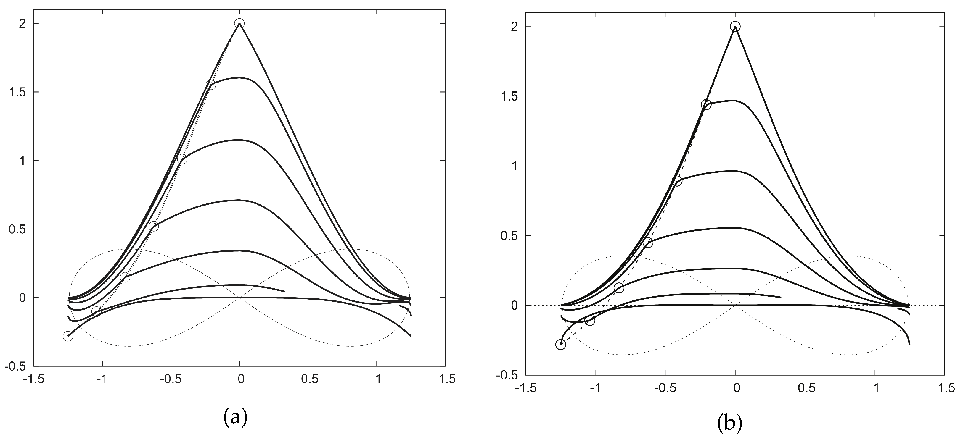
A comparison of the original two-dimensional Zakharov coefficient with the generalized coefficient on the resonance manifold was carried out by Dr. V.V. Geogjaev. Panels (a) and (b) in Figure 1 show the behavior of coefficients on the Phillips curve, respectively. In all curves, the coefficients are normalized: (). A quadruplet is defined by choosing two points P and on the Phillips curve. The curves in panels are built depending on the x coordinate of point while P is fixed for each curve.
Since the models are equivalent in the one-dimensional case, we assume that discrepancies in the dynamics between the proposed two-dimensional models and the Zakharov equation will appear when the dependence on the parameter increases. Nevertheless, the comparison showed that these discrepancies are small, and the coefficients are very similar, which justifies the generalization. The feature is that it is still possible to write the equation of motion in x space using , which is not possible if using the original Zakharov coefficient.
Now function depends on two space variables and time, operator corresponds to multiplication by , —to multiplication by in k space, and partial derivatives are replaced by ∇ operators.
Furthermore, in Section 3.1, we present the results obtained using this equation.
2.2. Generalization to Two-Dimensional Waves in Variables and
Let us generalize Hamiltonian (20) to the case of two-dimensional waves. For this purpose, we need to redefine all one-dimensional operators in the Hamiltonian. Recall that in the one-dimensional case, operator acts as a multiplication by in Fourier-space while acts as a multiplication by . Now we replace scalar k with a vector . Then, the operators are redefined as follows: , , and in k space. Operators and now turn to or and or , respectively. Furthermore, considering that , , now the Hamiltonian is:
The corresponding equations of motion are:
After taking the variation of the Hamiltonian, one can obtain a system of supercompact equations generalized for two-dimensional waves:
In addition to Hamiltonian (24), this system of equations has the following integrals of motion: the number of waves propagating to the “left” and to the “right” (with respect to ), longitudinal and transverse momentum.
The results of numerical simulations obtained by using Equation (25) will be shown in Section 3.2.
3. Numerical Simulations
The validity of the models is also confirmed by using the method of frozen coefficients. One can easily show that equations do not have instability at small scales, which is important in numerical simulations because of rounding errors. Both models (23) and (25) contain non-local terms with operator . Recall that this operator can be easily calculated in Fourier-space as multiplication by . Therefore, it seems reasonable to use pseudo-spectral Fourier methods to calculate the right-hand side of the equations. We use the standard fourth-order Runga–Kutta method for time integration. The correctness of the calculations is carried out by checking the conservation of the integrals of motion. The FFTW3 library [25] was used for the fast Fourier transform procedure. The multiplication of grid functions was carried out in x space, and the direct and inverse Fourier transforms were used to calculate derivatives and non-local terms. OpenMP tools were used to parallelize the numerical algorithm, and the 2D Fourier transforms paralleling was performed using the fftw3-threads.
To test the proposed models for adequacy in describing the dynamics of two-dimensional deep water waves, we consider the physical problem of standing waves in a channel with smooth vertical walls in our numerical simulations. For this purpose, we consider the periodic domain in the water channel with sizes m m. A perturbed one-dimensional standing wave with a characteristic wavelength m was considered as the initial condition. Average steepness . The perturbation was performed in the region around the basic harmonic . To prevent wave overturning, damping concentrated in the region of short wave harmonics was used.
Considering perturbed standing waves in a water channel with smooth vertical walls, it is necessary to make the surface derivative equal to zero at the walls. This means that the expansion of has to only contain cosines.
In terms of b and , the surface can be recovered by the following canonical transformations:
This results in the following conditions for variables:
Thus, condition (30) for b variables is maintained at each time step while calculating in Equation (23). In the case of variables , one can only use the first equation in (25) with condition (30) for variables:
The following sections will show the results of numerical simulations obtained within the framework of the proposed models.
3.1. Numerical Results Obtained in b Variable Model
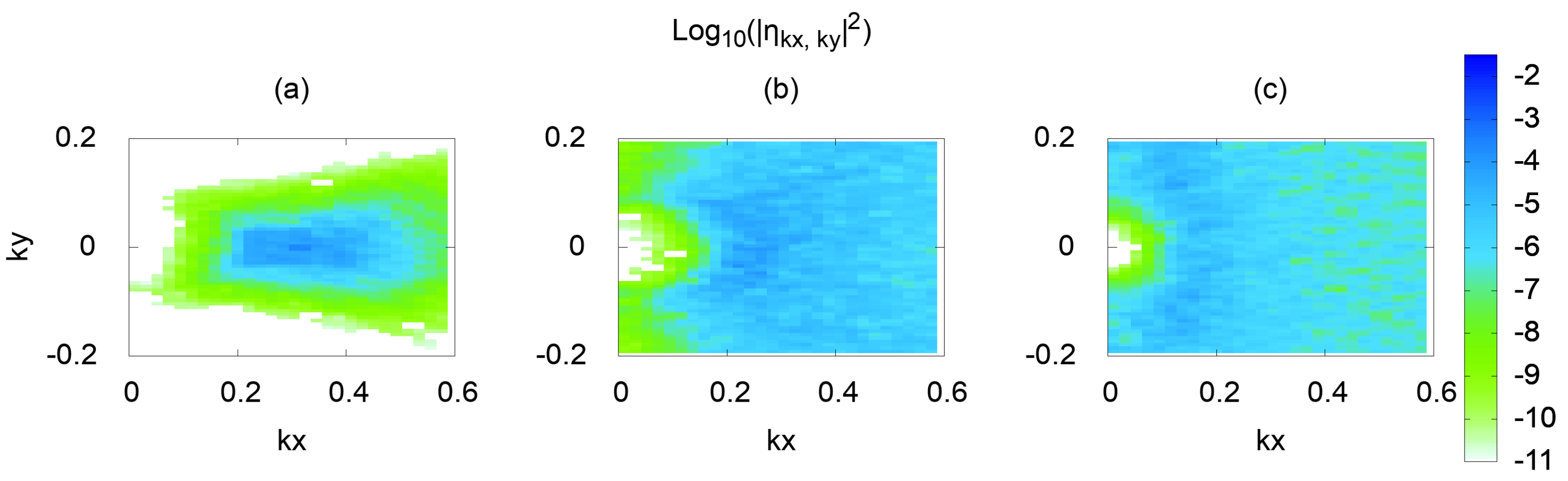
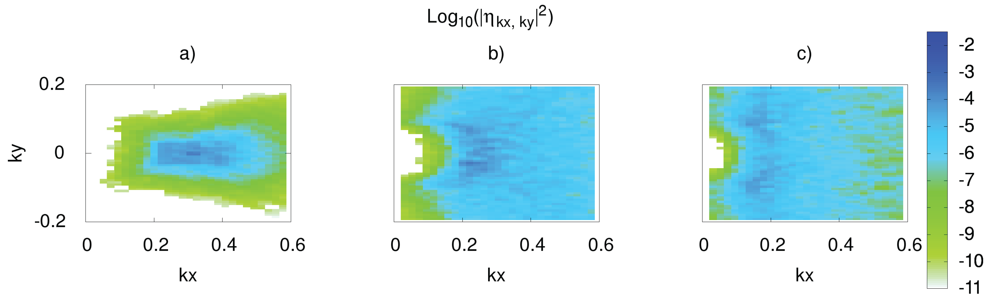
Figure 2 shows the two-dimensional spectra of at different times. The spectrum is symmetric with respect to the vertical line at since considering standing waves. That is why we do not show the part of the spectrum with negative . As it mentioned previously, initially (panel a) it is a one-dimensional standing wave with and small perturbation around it. In the process of time evolution, the spectrum expands (panel b) and eventually becomes almost isotropic (ring formation) after a long time (panel c).
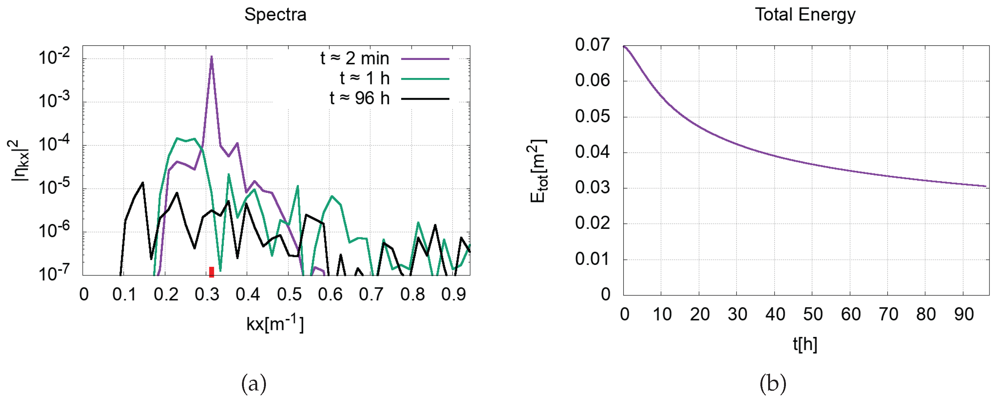
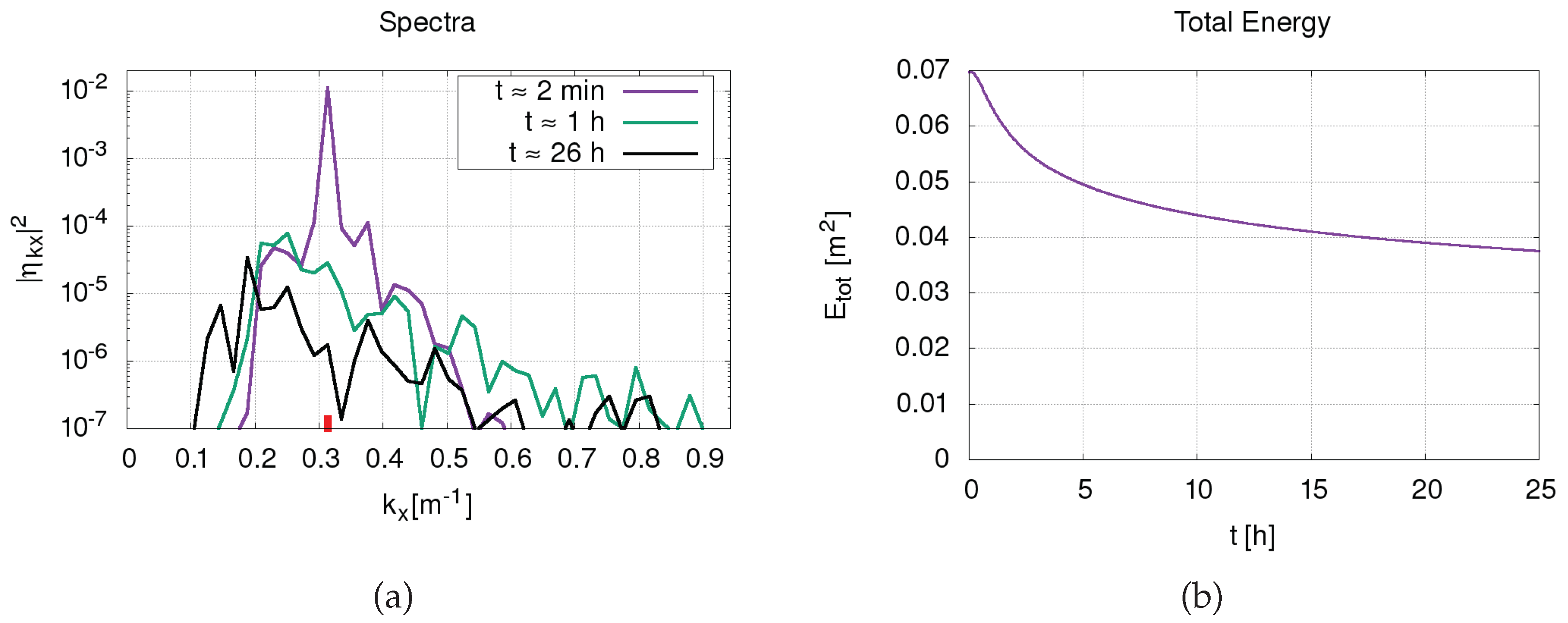
Figure 3 shows one-dimensional spectra at (panel a) and the dependence of total energy on time (panel b). It can be seen that the spectrum shifts to the region of long-wave harmonics with time; that is, the waves in the channel become longer along the x axis. Taken together with the two-dimensional spectrum, one can conclude that the waves become slightly longer in the x axis direction and significantly longer in the y axis direction. The total energy of the system gradually decreases due to the damping concentrated in the region of short-wave harmonics. It can be seen that the energy was almost halved in 96 h.
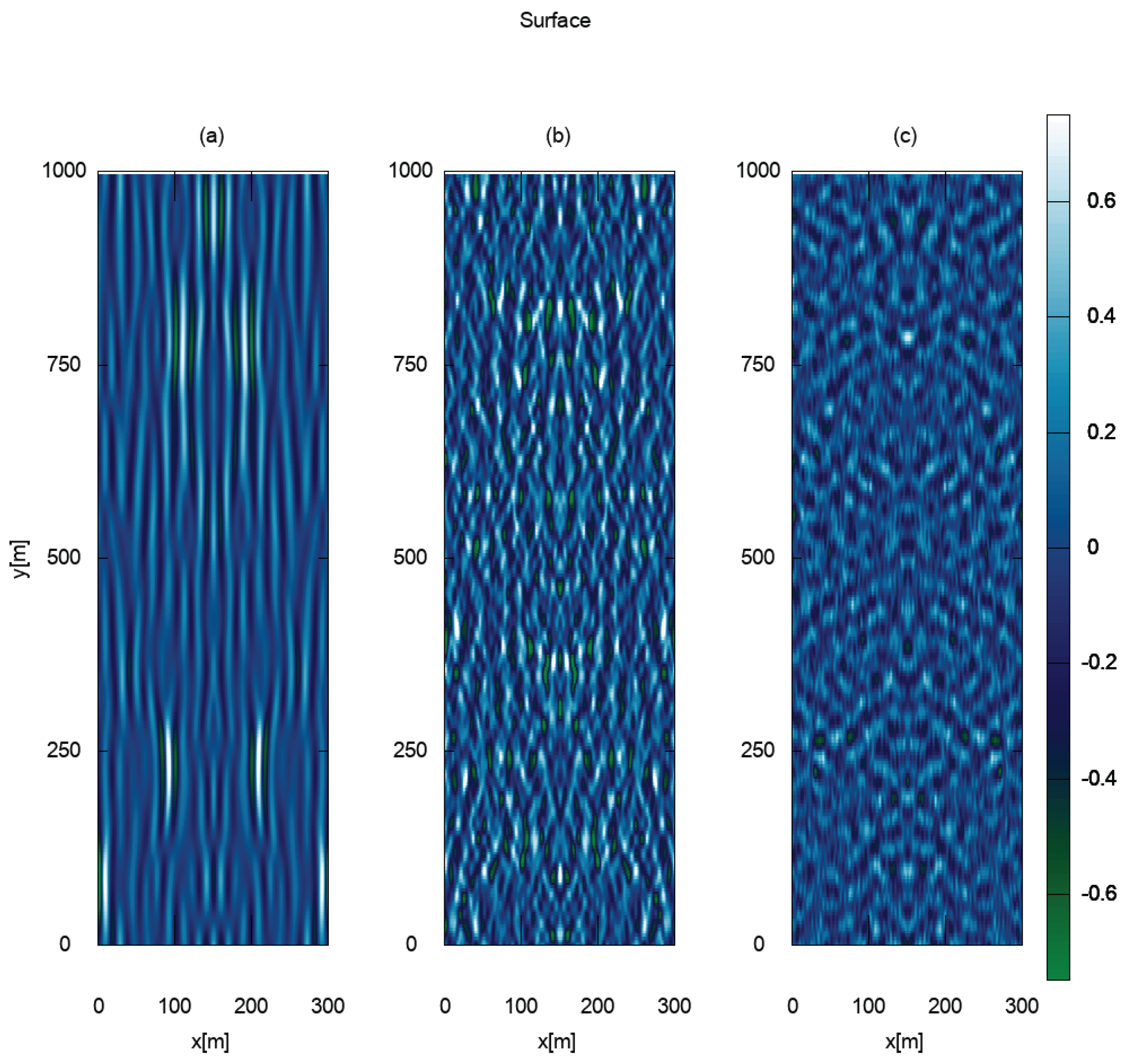
The time evolution of the surface is presented in Figure 4. The pictures are symmetrical around the central vertical line at m. In the beginning, the waves look quasi-one-dimensional. Then, the waves begin to bend over time. Finally, after a long time, the isotropization of the spectrum results in waves pointed in all directions.
Several films are available for more information:
A film with the dynamics of the one-dimensional spectrum can be viewed here: http://kachulin.itp.ac.ru/mdpi-2022-films/spectrum-1d.avi (accessed on 25 April 2022).
A film with the dynamics of the two-dimensional spectrum can be viewed here: http://kachulin.itp.ac.ru/mdpi-2022-films/spectrum-2d-zoom.avi (accessed on 25 April 2022).
Short films with surface dynamics are presented here.
At initial time: http://kachulin.itp.ac.ru/mdpi-2022-films/surface-0s.avi (accessed on 25 April 2022).
At final time: http://kachulin.itp.ac.ru/mdpi-2022-films/surface-96h.avi (accessed on 25 April 2022).
3.2. Numerical Results Obtained in the Model of and Variables
The model in terms of and slightly differs from the one in terms of b. Nevertheless, the detailed discussion of the results in Section 3.1 maintains its validity here as well. In Figure 5, one can also see the process of spectrum isotropization with time. Despite the differences, in general, the dynamics remain the same.
The same can be said about the one-dimensional spectrum shown in Figure 6 (panel a). Since the equations of motion in the and variables are different, the damping function is also different. This results in a change in energy dependence. It decreased more in the shorter computation time (panel b), but it did not again affect the overall dynamics.
Figure 7 presents the time evolution of the surface. Comparing panels (a) and (b) in Figure 4 and Figure 7, one can see that they are almost indistinguishable. Since there were no changes in the dynamics, the final computation time in this model was shorter.
A similar problem was considered in [26] in the framework of the equations in physical variables and corresponding to the Hamiltonian (3). It was shown that the initial spectrum of the perturbed standing wave becomes isotropic over time, and a specific ”ring” is formed. We observe very similar dynamics in proposed equations which can be clearly seen in Figure 2c and Figure 5c.
4. Conclusions
This work was devoted to the study of the hydrodynamics of two-dimensional waves propagating on the surface of a three-dimensional ideal incompressible fluid. Two new Hamiltonian models were proposed to describe the dynamics of such waves. The derivation of the models was based on the use of compact forms of the Zakharov equation for one-dimensional waves. Furthermore, we considered the dynamics of standing waves in a channel with smooth vertical walls as a physical problem. The results of numerical simulations showed an isotropization of the spectrum over time in both proposed models, which is entirely consistent with the studies carried out earlier. Furthermore, similarities in the overall dynamics in both models allowed us to conclude that the system of super-compact equations, which is the simplest form of the Zakharov equation, can be successfully applied to numerical simulations of two-dimensional deep water waves as well.
Author Contributions
Investigation, writing—review and editing, S.D., D.K. and A.D.; visualization, S.D. and D.K.; writing—original draft preparation, S.D., D.K. and A.D. All authors have read and agreed to the published version of the manuscript.
Funding
Section 2 and Section 3, excluding Section 2.2 and Section 3.2 of this research, were funded by the Russian Science Foundation Grant No. 19-72-30028, whilst Section 2.2 and Section 3.2 were funded by the Russian Foundation for Basic Research Grant No. 20-31-90093.
Institutional Review Board Statement
Not applicable.
Informed Consent Statement
Not applicable.
Data Availability Statement
Not applicable.
Acknowledgments
We are grateful to V.V. Geogjaev for providing results that improved this article. Numerical simulations were performed at the Novosibirsk Supercomputer Center of Novosibirsk State University and at the computing cluster of Landau Institute for Theoretical Physics RAS.
Conflicts of Interest
The authors declare no conflict of interest concerning the paper.
Abbreviations
The following abbreviations are used in this manuscript:
| NLSE | Nonlinear Schrödinger equation |
| HOSM | High-order spectral method |
References
- Ablowitz, M.J.; Kaup, D.J.; Newell, A.C.; Segur, H. The inverse scattering transform-Fourier analysis for nonlinear problems. Stud. Appl. Math. 1974, 53, 249–315. [Google Scholar] [CrossRef]
- Zakharov, V.E.; Manakov, S. On the complete integrability of a nonlinear Schrödinger equation. Theor. Math. Phys. 1974, 19, 551–559. [Google Scholar] [CrossRef]
- Zakharov, V.E. Stability of periodic waves of finite amplitude on the surface of a deep fluid. J. Appl. Mech. Tech. Phys. 1968, 9, 190–194. [Google Scholar] [CrossRef]
- Dyachenko, A.I.; Zakharov, V.E. Compact equation for gravity waves on deep water. JETP Lett. 2011, 93, 701–705. [Google Scholar] [CrossRef]
- Dyachenko, A.; Kachulin, D.; Zakharov, V. Super compact equation for water waves. J. Fluid Mech. 2017, 828, 661–679. [Google Scholar] [CrossRef] [Green Version]
- West, B.J.; Brueckner, K.A.; Janda, R.S.; Milder, D.M.; Milton, R.L. A new numerical method for surface hydrodynamics. J. Geophys. Res. Ocean. 1987, 92, 11803–11824. [Google Scholar] [CrossRef]
- Dyachenko, A.I.; Kuznetsov, E.A.; Spector, M.; Zakharov, V.E. Analytical description of the free surface dynamics of an ideal fluid (canonical formalism and conformal mapping). Phys. Lett. A 1996, 221, 73–79. [Google Scholar] [CrossRef]
- Dyachenko, A.I. On the dynamics of an ideal fluid with a free surface. Dokl. Math. 2001, 63, 115–117. [Google Scholar]
- Ruban, V.P. Quasiplanar steep water waves. Phys. Rev. E 2005, 71, 055303. [Google Scholar] [CrossRef] [Green Version]
- Ruban, V.P.; Dreher, J. Numerical modeling of quasiplanar giant water waves. Phys. Rev. E 2005, 72, 066303. [Google Scholar] [CrossRef] [Green Version]
- Ruban, V.P. Breathing rogue wave observed in numerical experiment. Phys. Rev. E 2006, 74, 036305. [Google Scholar] [CrossRef] [PubMed] [Green Version]
- Ruban, V.P. Conformal variables in the numerical simulations of long-crested rogue waves. Eur. Phys. J. Spec. Top. 2010, 185, 17–33. [Google Scholar] [CrossRef]
- Davey, A.; Stewartson, K. On three-dimensional packets of surface waves. Proc. R. Soc. Lond. Math. Phys. Sci. 1974, 338, 101–110. [Google Scholar]
- Hui, W.; Hamilton, J. Exact solutions of a three-dimensional nonlinear Schrödinger equation applied to gravity waves. J. Fluid Mech. 1979, 93, 117–133. [Google Scholar] [CrossRef]
- Yuen, H.C.; Lake, B.M. Nonlinear dynamics of deep-water gravity waves. Adv. Appl. Mech. 1982, 22, 67–229. [Google Scholar]
- Dysthe, K.B. Note on a modification to the nonlinear Schrödinger equation for application to deep water waves. Proc. R. Soc. London. Math. Phys. Sci. 1979, 369, 105–114. [Google Scholar]
- Trulsen, K.; Kliakhandler, I.; Dysthe, K.B.; Velarde, M.G. On weakly nonlinear modulation of waves on deep water. Phys. Fluids 2000, 12, 2432–2437. [Google Scholar] [CrossRef]
- Kokorina, A.; Slunyaev, A. Lifetimes of rogue wave events in direct numerical simulations of deep-water irregular sea waves. Fluids 2019, 4, 70. [Google Scholar] [CrossRef] [Green Version]
- Slunyaev, A.; Kokorina, A. Account of occasional wave breaking in numerical simulations of irregular water waves in the focus of the rogue wave problem. Water Waves 2020, 2, 243–262. [Google Scholar] [CrossRef] [Green Version]
- Hasselmann, K. On the non-linear energy transfer in a gravity-wave spectrum Part 1. General theory. J. Fluid Mech. 1962, 12, 481–500. [Google Scholar] [CrossRef]
- Zakharov, V. Analytic theory of a wind-driven sea. Procedia IUTAM 2018, 26, 43–58. [Google Scholar] [CrossRef]
- Zakharov, V.E.; Badulin, S.I.; Geogjaev, V.V.; Pushkarev, A.N. Weak-turbulent theory of wind-driven sea. Earth Space Sci. 2019, 6, 540–556. [Google Scholar] [CrossRef]
- Geogjaev, V.; Zakharov, V.E. Numerical and analytical calculations of the parameters of power-law spectra for deep water gravity waves. JETP Lett. 2017, 106, 184–187. [Google Scholar] [CrossRef]
- Dyachenko, A.I. Canonical system of equations for 1D water waves. Stud. Appl. Math. 2020, 144, 493–503. [Google Scholar] [CrossRef]
- Frigo, M.; Johnson, S.G. The design and implementation of FFTW3. Proc. IEEE 2005, 93, 216–231. [Google Scholar] [CrossRef] [Green Version]
- Korotkevich, A.O.; Dyachenko, A.I.; Zakharov, V.E. Numerical simulation of surface waves instability on a homogeneous grid. Phys. D Nonlinear Phenom. 2016, 321, 51–66. [Google Scholar] [CrossRef] [Green Version]
Figure 1.
Behavior of in panel (a) and in panel (b) depending on at fixed P. Each curve has a circle corresponding to the x coordinate of point P. The circles form a curve for matching vectors . The left part of the panels corresponds to P and which are in the same quadrant while the right part corresponds to the case wherein P and are in different quadrants.

Figure 2.
The evolution of spectrum in time in logarithmic scale. The color shows the squared amplitude of the harmonic. Panel (a) corresponds to the almost initial surface at time min. Panel (b) corresponds to the surface at time h, and panel (c) corresponds to the surface at time h.
Figure 2.
The evolution of spectrum in time in logarithmic scale. The color shows the squared amplitude of the harmonic. Panel (a) corresponds to the almost initial surface at time min. Panel (b) corresponds to the surface at time h, and panel (c) corresponds to the surface at time h.

Figure 3.
Panel (a) shows the evolution of one-dimensional spectrum overtime in logarithmic scale. A small red line indicates the initial characteristic wavenumber . Purple curve corresponds to the almost initial spectrum at time min, green curve corresponds to the spectrum at time h, and the black one corresponds to the spectrum at time h. Panel (b) shows the total energy dependence in time.

Figure 4.
The evolution of surface in time. The color shows the amplitude of the waves in meters. Panel (a) corresponds to the almost initial surface at time min. Panel (b) corresponds to the surface at time h, and Panel (c) corresponds to the surface at time h.
Figure 4.
The evolution of surface in time. The color shows the amplitude of the waves in meters. Panel (a) corresponds to the almost initial surface at time min. Panel (b) corresponds to the surface at time h, and Panel (c) corresponds to the surface at time h.

Figure 5.
The evolution of spectrum in time in logarithmic scale. The color shows the squared amplitude of the harmonic. Panel (a) corresponds to the almost initial surface at time min. Panel (b) corresponds to the surface at time h, and Panel (c) corresponds to the surface at time h.
Figure 5.
The evolution of spectrum in time in logarithmic scale. The color shows the squared amplitude of the harmonic. Panel (a) corresponds to the almost initial surface at time min. Panel (b) corresponds to the surface at time h, and Panel (c) corresponds to the surface at time h.

Figure 6.
Panel (a) shows the evolution of one-dimensional spectrum in time in logarithmic scale. A small red line indicates the initial characteristic wavenumber . Purple curve corresponds to the almost initial spectrum at time min, green curve corresponds to the spectrum at time h, and the black one corresponds to the spectrum at time h. Panel (b) shows the dependence of total energy in time.

Figure 7.
The evolution of surface in time. The color shows the amplitude of the waves in meters. Panel (a) corresponds to the almost initial surface at time min. Panel (b) corresponds to the surface at time h, and Panel (c) corresponds to the surface at time h.
Figure 7.
The evolution of surface in time. The color shows the amplitude of the waves in meters. Panel (a) corresponds to the almost initial surface at time min. Panel (b) corresponds to the surface at time h, and Panel (c) corresponds to the surface at time h.

Publisher’s Note: MDPI stays neutral with regard to jurisdictional claims in published maps and institutional affiliations. |
© 2022 by the authors. Licensee MDPI, Basel, Switzerland. This article is an open access article distributed under the terms and conditions of the Creative Commons Attribution (CC BY) license (https://creativecommons.org/licenses/by/4.0/).
Share and Cite
MDPI and ACS Style
Dremov, S.; Kachulin, D.; Dyachenko, A. Two Models for 2D Deep Water Waves. Fluids 2022, 7, 204. https://0-doi-org.brum.beds.ac.uk/10.3390/fluids7060204
AMA Style
Dremov S, Kachulin D, Dyachenko A. Two Models for 2D Deep Water Waves. Fluids. 2022; 7(6):204. https://0-doi-org.brum.beds.ac.uk/10.3390/fluids7060204
Chicago/Turabian StyleDremov, Sergey, Dmitry Kachulin, and Alexander Dyachenko. 2022. "Two Models for 2D Deep Water Waves" Fluids 7, no. 6: 204. https://0-doi-org.brum.beds.ac.uk/10.3390/fluids7060204