
Hydrodynamic Interaction of Two Self-Propelled Fish Swimming in a Tandem Arrangement


Department of Aerodynamics, Nanjing University of Aeronautics and Astronautics, Yudao Street 29, Nanjing 210016, China
*
Author to whom correspondence should be addressed.
†
These authors contributed equally to this work.
‡
Current address: Key Laboratory of Unsteady Aerodynamics and Flow Control, Ministry of Industry and Information Technology, Nanjing University of Aeronautics and Astronautics, Yudao Street 29, Nanjing 210016, China.
Fluids 2022, 7(6), 208; https://0-doi-org.brum.beds.ac.uk/10.3390/fluids7060208
Submission received: 15 May 2022
/
Revised: 14 June 2022
/
Accepted: 15 June 2022
/
Published: 17 June 2022
(This article belongs to the Special Issue Fluid–Structure Interaction in Biological, Bioinspired and Environmental Flows)
Abstract
:Collective locomotion in biological systems is ubiquitous and attracts much attention, and there are complex hydrodynamics involved. The hydrodynamic interaction for fish schooling is examined using two-dimensional numerical simulations of a pair of self-propelled swimming fish in this paper. The effects of different parameters on swimming speed gain and energy-saving efficiency are investigated by adjusting swimming parameters (initial separation distance , tail beat amplitude A, body wavelength , and period of oscillation T) at different phase difference between two fish. The hydrodynamic interaction performance of fish swimming in a tandem arrangement is analyzed with the help of the instantaneous vorticity contours, pressure contours, and mean work done. Using elementary hydrodynamic arguments, a unifying mechanistic principle, which characterizes the fish locomotion by deriving a scaling relation that links swimming speed u to body kinematics (A, T, and ), arrangement of formation (), and fluid properties (kinematic viscosity ), is revealed. It is shown that there are some certain scaling laws between similarity criterion number (Reynolds number (Re) and Strouhal number ()) and energy-consuming coefficient () under different parameters (). In particular, a generality in the relationships of –Re and –(Re ) can emerge despite significant disparities in locomotory performance.
1. Introduction
Schooling is a common phenomenon in fish creatures [1], and the cluster movement of specific formations can significantly improve the swimming efficiency of fish schooling. The study of the energy-saving mechanism of fish schooling swimming provides inspiration and helps in the design and control of robot cluster formation, which has been receiving wide concern from researchers. A great aspect of fish swimming is to make use of the surrounding environment for efficient propulsion. Due to this fact, many species in fish tend to swim in the form of groups, known as schools. Extensive studies have shown that fish schooling is generally more efficient than swimming alone, with more than 50% of fish in nature showing synchronized and coordinated schooling swimming at some time [2]. Many fish swim in the same direction in schooling and maintain the near-constant spacing with neighboring counterparts when they migrate [3]. In addition to sociological advantages such as avoiding natural enemies [4,5] and improving predation success rate [6], schooling swimming is also believed to effectively reduce energy consumption [7,8]. Various schooling patterns are observed in fish swimming [7] that include line, diamond, triangular, and phalanx formations [9]. The advantage of these congregations lies in the fact that each fish tends to gain energy from surrounding vortical flows generated by neighboring bodies.
At present, there are many studies on self-propelled schooling, including flexible body and rigid flapping wing [10,11,12,13,14,15,16,17], and they reveal the energy-saving mechanism of schooling swimming. Meanwhile, multi-party flow-mediated interaction has been widely observed in swimming fish. The inviscid theoretical model of Weihs [1] demonstrated that trailing fish in a diamond configuration could benefit from the reduced flow induced by the oncoming vortices. Herskin and Steffensen [18] observed that the tail-beat frequency of trailing fish was lower than that of fish at the front of the school. Moreover, Killen et al. [8] noted that fish with inherently lower aerobic scope preferred to stay towards the rear of a group. Marras et al. [19] found that both the upstream and rear fish saved energy regardless of their positions. Although many recent experimental studies have shown the hydrodynamic benefits of fish schools [8,18,19,20], the question of which schooling structures are optimal from a hydrodynamic point of view is still controversial, and an in-depth understanding of the hydrodynamic mechanisms by which fish schools benefit from flow-mediated interactions is desirable.
In this paper, we use a computational model of a swimming fish in a tandem arrangement to understand the hydrodynamic mechanisms by which fish schools benefit from flow-mediated interactions. Two fish swimming with a flexible body, based on the kinematic mechanics of the carangiform swimmer, are simulated. An adaptive immersed boundary (IB) method proposed by Bhalla et al. [21] is adopted to handle the fish swimming. The IB method has been extensively applied for various fluid–structure interaction (FSI) simulations [22,23,24,25]. To gain deeper understanding and knowledge of fish-schooling mechanisms, it is very important to investigate what benefits the upstream and rear fish find in these situations and what mechanisms they follow. To study the effect of the presence of a body swimming asynchronously to another body in its vicinity, the hydrodynamic interaction performance of fish swimming in a tandem arrangement is analyzed with the help of the instantaneous vorticity contours, pressure contours, and mean work done. The remainder of this paper is organized as follows. Section 2 provides details of the numerical methodology, kinematic modeling, boundary conditions, and calculation of correlation formula employed. In Section 3, the results and discussions of current research are presented. Section 4 concludes this study and shows some prospects to the future work.
2. Problem Description and Methods
In this section, the fish kinematics and the computational details are described in Section 2.1, the formulations for calculating hydrodynamic arguments and correlation formula are provided in Section 2.2, and the numerical method is presented in Section 2.3.
2.1. Fish Body Kinematics and Computational Details
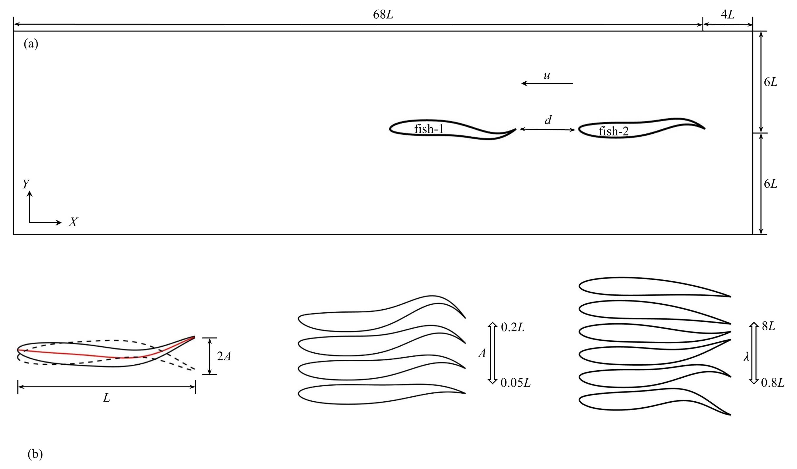
In this study, two identical fish-like NACA0012 foils self-propel from the right to left side of computational domain, and the fish are allowed to move in a horizontal (x) direction. Figure 1 presents a sketch of computational domain with two fish in tandem arrangement, and the fish parameters are also involved. As shown in Figure 1a, two fish swim along the x-direction by creating undulatory motion in the y-direction. As presented in Figure 1b, the fish length is L, and the tail beat amplitude of the fish is A. The kinematics for carangiform swimmers is usually in the form of a backward traveling wave with the largest wave amplitude at the fish tail. To account for the traveling wave, the displacement of the midline of fish from the x-axis is given by
where is the time-wise, as well as stream-wise, varying lateral displacement of the fish centerline, x is the axial direction measured along the fish axis from the tip of the fish head, t is the time, i = 1, 2 represent the upstream fish and rear fish in the tandem formation, respectively. is the stream-wise linearly varying amplitude function (A = is the maximum amplitude at the tail when x = L), k = 2/ is the wave number of the body undulation that is related to the wavelength , = 2 is the angular frequency that is related to the tail beat frequency f, and is the initial phase. The phase difference is defined as .
The amplitude function can be represented by a quadratic curve of the form:
where the coefficients , and are chosen as = 0.02, = −0.08 and = 0.16, respectively, which are the same as the work of Wang and Wu [26].
Two important similarity parameters in fish swimming are the Reynolds number and the Strouhal number, which are defined as:
where is the mean swimming speed of fish, and is the kinematic viscosity of fluid, In this study, Re and are in the ranges of [2897, 13513] and [0.13, 0.25], respectively.
The size of computational domain is 72L × 12L. The periodic boundary conditions are applied to the left and right sides of domain, and no-slip boundary conditions are used for the upper and lower sides of domain. The head of the rear fish is initially centered at = (0, 0), and its body extends in the positive x-direction. Moreover, “fish-1” and “fish-2” represent the upstream fish and the rear fish in a tandem arrangement, respectively.
In this study, the settings of swimming parameters are as follows. The initial separation distance between two fish is = 0.1L–1.0L, the tail beat amplitude is A = 0.05L–0.2L with the interval of = 0.05L, the wavelength is = 0.8L–8L and the period of oscillation (T = 1/f) is T = 0.5–2.0 with the interval of = 0.25, in which = 1.0 s is the set characteristic period of oscillation. All the parameters in this study use the physical units, and please refer to the abbreviations table at the end of the paper for more details.
2.2. Calculation of Hydrodynamic Arguments and Correlation Formula
The swimming speed is calculated based on the hydrodynamic forces acting on the fish body using Newton’s second law of motion [27], which is governed by:
where m is the total mass of the fish body, u is the swimming speed, and is net force on the fish body in the x-direction. Swimming creatures move based on the undulating kinematics of their bodies, and the body undulation is predominantly in a direction lateral to the swimming direction [28,29,30,31]. The power of swimming is calculated by:
where V is the volume of the constrained fish body, and is the density of the constrained fish body, which equals to the fluid density in this study. is the constrained Lagrangian body velocity field, and is the constraint force density. More details can be referred to Ref. [21]. The mean net power spent is governed by [32]:
where is the fluctuation quantity of swimming speed, and is the mean lateral power spent quantity.
The energy efficiency of the swimmers in the tandem arrangement can be quantified by the cost of transport per unit mass (), which is defined as the energy required for a unit mass to travel a unit distance:
Whereas the dimensionless measure is preferred to enable comparison of efficiency of swimmers across species and length scales, the scaling of follows from the ratio of the scaling of power spent to the scaling of speed [32] is then adopted:
where is the density of the fluid. In this work, the relative difference of between a fish in formation swimming and that in solitary swimming is used to describe energy-saving efficiency, which can be governed by:
where the subscript ‘s’ denotes solitary swimming.
To explain the variation of energy-saving efficiency in the tandem arrangement, the mean work done during fish swimming is calculated:
and then the power coefficient is defined as:
2.3. Numerical Method
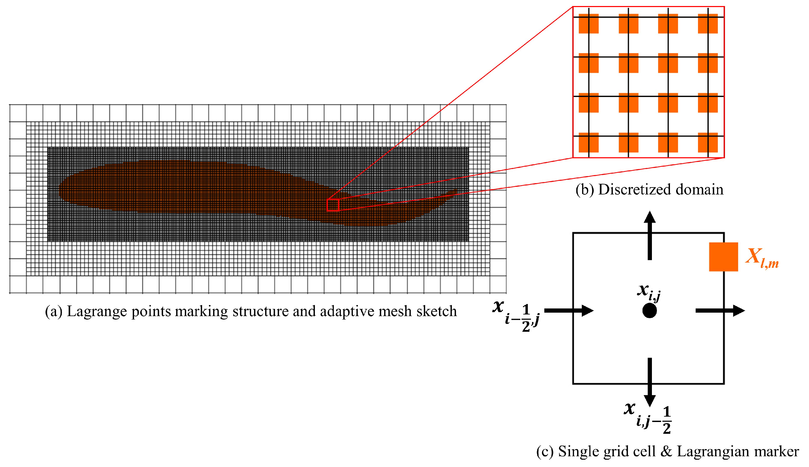
In this work, the IB method together with adaptive mesh refinement (IBAMR) [21,33] is employed to deal with the fish motion. The hydrodynamic approach version of IB method has been used. This IB method is suitable for problems in which the aim is to determine swimming velocities or forces generated during swimming. The deformational kinematics data required by the hydrodynamic approach to simulating aquatic locomotion can be obtained from experiments [28,34,35,36,37,38,39]. The IB formulation uses an Eulerian description for the momentum equation and divergence-free condition for both the fluid and the structure. A Lagrangian description is employed for the structural position and forces, more details refer to [40]. IBAMR relies on SAMRAI [41,42,43] for Cartesian grid management and the adaptive mesh refinement [44,45,46] framework. Solver support in IBAMR is provided by PETSc library [47]. Adopting IB method permits us to avoid body conforming mesh discretization and to use fast Cartesian grid solvers. The effect of the fish body on the fluid is implemented via an additional body force that is added to the (fluid) momentum equation. The Cartesian grid adaptive mesh refinement is applied for the fish motion, and thereby the thin boundary layers at fluid-solid interfaces as well as flow structures shed from such interfaces can be captured efficiently. The numerical method adopted has been applied successfully to simulate fish-like swimming problems [25,48,49,50,51,52,53,54]. In this study, the fish body structure is marked by Lagrangian points and then Lagrangian discretization. Quantities attached to the structure are described in a Lagrangian frame on immersed markers that are free to arbitrarily cut through the background Cartesian mesh. These nodes are indexed by (l, m) with curvilinear mesh spacing (, ), each cell center of the grid has position = ((), ()) for i = 0,…, 1, j = 0,…, 1. For a given cell (i, j), = (, ()) is the physical location of the cell face that is half a grid space away from in the x-direction, = ((), ) is the physical location of the cell face that is half a grid cell away from in the y-direction, and the position of a marker point is denoted as . A staggered grid discretization for quantities described in the Eulerian frame was adopted, and refer readers to [55] for more details. Figure 2 gives a sketch of the spatial discretization. The computational domain is discretized using an adaptively refined grid for which the finest grid resolution is = = 0.0026L. The time step size is taken to be = 0.0005T. More information on the grid and time-step independence tests can be found in the Supplementary Material S1, and further convergence studies of IB method have been published in previous work [21,52,55].
3. Results and Discussion
In this section, the hydrodynamic characteristics of two fish swimming in a tandem arrangement with different swimming parameters are discussed in Section 3.1, and the scaling laws for Reynolds number, Strouhal number, and ratio of the scaling of power spent to the scaling of speed are discussed in Section 3.2.
3.1. Effects of Swimming Parameters on Hydrodynamics
3.1.1. Effect on Swimming Speed
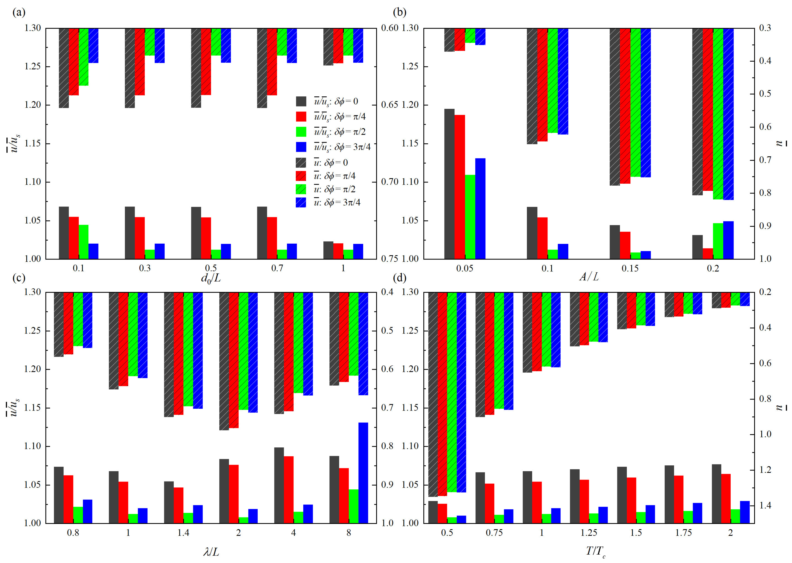
In the stable state, two fish have the same mean swimming speed, i.e., = = , where the subscripts “1” and “2” represent upstream fish and rear fish, respectively. The histogram comparisons of / and with different swimming parameters are provided in Figure 3, where is the mean swimming speed of isolated fish. The higher the value of / is, the higher the speed gain (the speed gain is calculated as ((−)/) × 100%) of two tandem fish with respect to the isolated fish. It can be seen from Figure 3 that except for the cases of larger tail beat amplitude, smaller initial separation distance and larger wavelength, the speed gain of two tandem fish shows a fixed trend under different phase differences. The maximum / appears at = 0, which is followed by = /4. Meanwhile, the minimum / appears at = /2, which is followed by = 3/4.
As shown in Figure 3a, the variation trend of / with is consistent with that of . In particular, for the cases of = 0 and /4, / is roughly unchanged when 0.1L⩽⩽ 0.7L, and the corresponding speed gains are 6.8% and 5.4%, respectively. Meanwhile, when = 1.0L, the speed gains for = 0 and /4 are 2.3% and 2.1%, respectively. On the other hand, for the case of = /2, the maximum / appears at = 0.1L, and the speed gain is 4.4%. When 0.3L⩽⩽ 1.0L, / is roughly unchanged, and the speed gain is 1.2%. However, for the case of = 3/4, / is independent of , and the speed gain is 2.0%.
As shown in Figure 3b, for the cases of = 0 and /4, / decreases with the increase of A. At = 0, the speed gains at four tail beat amplitudes are 19.5%, 6.8%, 4.4% and 3.1%, respectively. At = /4, the corresponding speed gains are 18.7%, 5.4%, 3.5% and 1.4%, respectively. For the cases of = /2 and = 3/4, however, with the increase of A, / has a tendency of first decrease and then increase. When = /2, the corresponding speed gains are 11.0%, 1.2%, 0.8% and 4.7%, respectively. When = 3/4, the corresponding speed gains are 13.1%, 2.0%, 1.1% and 4.9%, respectively. Therefore, it is known that the larger tail beat amplitude does not represent the higher speed gain, and the speed gain is always the highest when A = 0.05L in this case. On the other hand, increases with A monotonically.
As shown in Figure 3c, the variation of / with respect to is complex. For the cases of = 0 and /4, the extreme values of / occur at the same wavelength, i.e., the maximum and minimum / appear at = 4L and = 1.4L, respectively. The corresponding speed gains are 9.9% and 5.4% when = 0, and 8.7% and 4.7% when = /4. Similarly, for the cases of = /2 and = 3/4, the maximum and minimum / appear at = 8L and = 2L, respectively. The corresponding speed gains are 13.1% and 1.9% when = 3/4, and 4.4% and 0.8% when = /2. However, different phase differences can generate the extreme values of at the same wavelength, and the maximum and minimum appear at = 2L and = 0.8L, respectively.
As shown in Figure 3d, it is shown that with the increase of T, the overall presents a decreasing trend. Instead, / increases with T. But when T⩾ 0.75, the increment of / is negligible. On the other hand, the maximum and minimum speed gains also appear at T = 2.0 and 0.5, respectively. Specific speed gains are 7.7% and 2.9% when = 0, 6.4% and 2.5% when = /4, 1.9% and 0.8% when = /2, and 2.8% and 0.9% when = 3/4. Table 1 gives the overview of speed gains with all studied parameters.
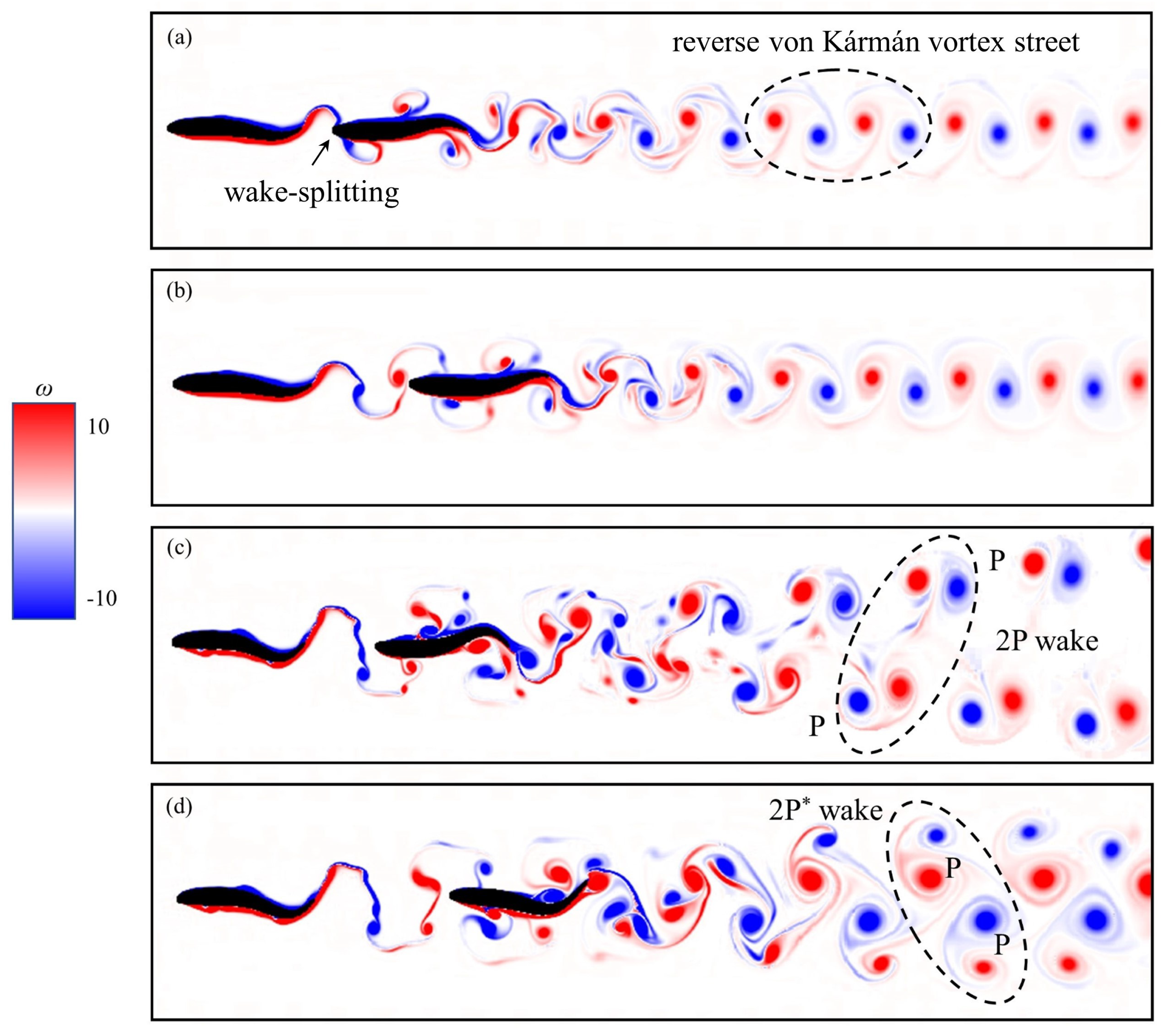
The results in Figure 3 may be explained through the interaction of two fishtail vortices. Some typical instantaneous vorticity contours are presented in Figure 4. The period of oscillation and wavelength are T = 1.0 and = 1.0L, respectively. For the case of = 0.1L, A = 0.1L and = /2, as shown in Figure 4a, the interaction of the rear fish with the vortices shed by the upstream fish as well as the wake developed in its downstream direction can be observed clearly. When the vortices shed by the upstream fish interact with the leading edge of the rear fish, they are split into two parts. This is the result of wake-splitting [56] at the leading edges of the rear fish, and both parts interact with shear layer around the fish body. For the case of = 0.1L, A = 0.1L and = 3/4, the vortices with small lateral width near the trailing edge are produced, as shown in Figure 4b. The wake-splitting phenomenon happens earlier at the leading edges of the rear fish when the vortices roll along upstream fish body and detach from upstream fish trailing edge. As a result, the concentrated vortices with high energy are shed into the rear fish. This can explain why the speed gain of two fish swimming at = /2 is higher than that of = 3/4 when = 0.1L and A = 0.1L. Similarly, the speed gain of two fish swimming at = /2 is higher than that of = /4 when = 0.5L and A = 0.2L, as shown in Figure 4c,d, respectively. Again, the reason that the speed gain of two fish swimming at = 3/4 is higher than that of = 0 when = 8L can be explained by using the same way.
Figure 4a,b also present the phenomenon of wake transformation from the von Kármán vortex street into the reverse von Kármán vortex street. It produces a momentum surfeit region in the near wake region of the body, and causes a negative drag, which is also termed as thrust force [57]. This is also a reason for the speed gain of tandem arrangement swimming. In Figure 4c,d, the vortex patterns of 2P and 2P [58,59] are formed, respectively. The 2P wake structure is believed to be responsible for the performance enhancement, and the propulsion mechanisms have been explained in previous work [60]. For the four cases in Figure 4, in order to observe the evolution of vortex in the process of motion more intuitively, the dynamic view of two fish swimming is presented in the Supplementary S2. Whether the form of vortex evolution is regularly correlated with swimming parameters, which needs to be further studied in the future.
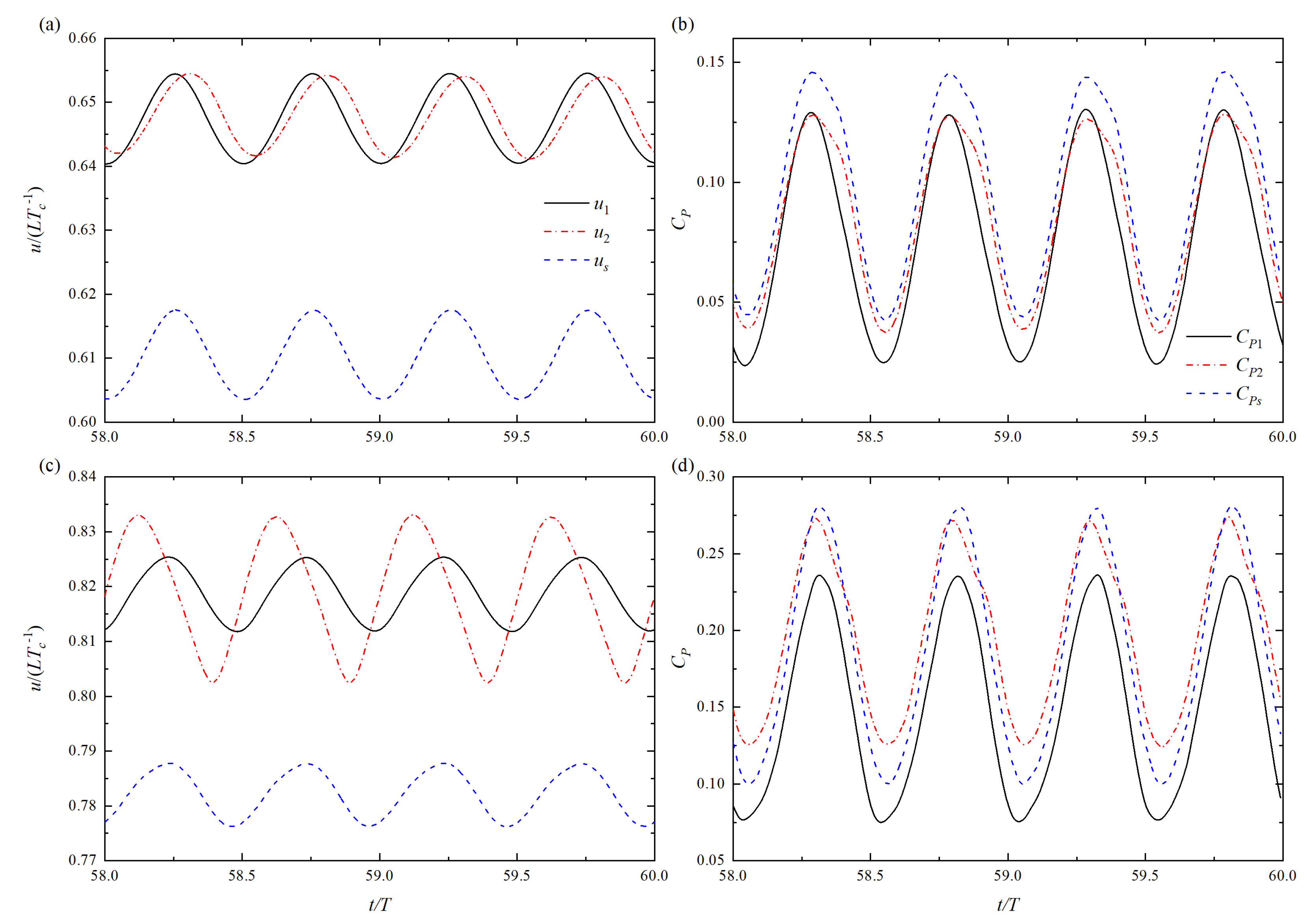
Figure 5 shows the time histories of swimming speed u and power coefficient at T = 1.0, = 1.0L and = /2. For the case of = 0.1L and A = 0.1L, there is a phase shift of u curve between the upstream fish and the rear fish, as shown in Figure 5a. The speed amplitude of the rear fish is smaller than that of the upstream fish. Compared with isolated fish, the amplitude and phase of u curve of upstream fish are basically identical. Meanwhile, the power coefficients of both fish in tandem formation are smaller than that of the isolated fish, as shown in Figure 5b. The relationship of the power coefficient is as follows: > > .
For the case of = 0.5L and A = 0.2L, there is also a phase shift of u curve between the upstream fish and the rear fish, as shown in Figure 5c. The speed amplitude of the rear fish is larger than that of the upstream fish. Similarly, u curve of upstream fish is hardly affected, as compared with the isolated fish. As can be observed from Figure 5d, the power coefficient still changes periodically. However, the power coefficient of the isolated fish is no longer greater than that of the rear fish in the tandem arrangement. The relationship of the power coefficient is as follows: > > . It is known that for the tandem arrangement, the speed waveform of the upstream fish is not affected basically.
3.1.2. Effect on Energy-Saving Efficiency
It is reasonable that two fish in the tandem arrangement can both reduce energy expenditure and improve swimming efficiency [61]. To investigate how the hydrodynamic interactions affect the energy behavior of fish swimming in the tandem arrangement, the energy-saving efficiency in swimming process is analyzed by cost of transport and the wake vortex interaction.
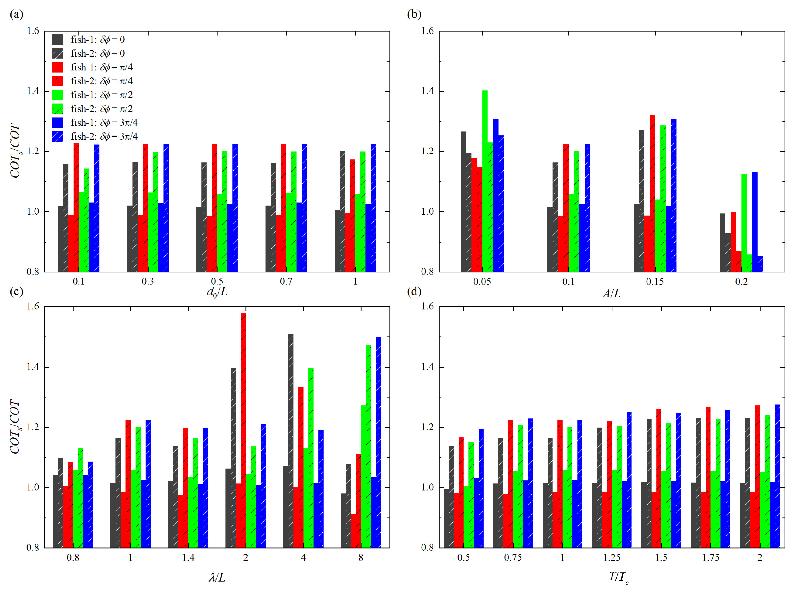
The ratio of the cost of transport of the isolated fish () to the cost of transport of a fish in tandem arrangement ( and ) is calculated to determine the energy saving. Since the lower value of is desirable that indicates lower energy consumption [62], so when / > 1, swimming is more energy-saving efficient, where in the denominator represents either of the upstream fish or of the rear fish. The histogram comparisons of / with different swimming parameters are given in Figure 6. It is found that except for the cases of larger and smaller tail beat amplitudes, the rear fish is always more energy-saving efficient than the upstream fish. Meanwhile, for the upstream fish, the maximum energy-saving efficiency appears at = /2, which is followed by = 3/4, and minimum energy-saving efficiency appears at = /4, which is followed by = 0.
As shown in Figure 6a, / is generally independent of . For the rear fish, the situation is more complex. When = 0, / is roughly unchanged during 0.1L⩽⩽ 0.7L, and the energy-saving efficiency is 14.1%, which becomes 16.8% at = 1.0L. When = /4, / is basically independent of in the range of 0.1L⩽⩽ 0.7L, and the energy-saving efficiency is 18.3%, which becomes 14.7% at = 1.0L. When = /2, / has a minimum value at = 0.1L, and the energy-saving efficiency is 12.5%, which can roughly keep at 16.7% during 0.3L⩽⩽ 1.0L. When = 3/4, / is basically independent of , and the energy-saving efficiency maintains at 18.3%. In addition, it is noted that the upstream fish consumes more energy than the isolated fish when = /4.
As shown in Figure 6b, the higher energy consumption occurs in the rear fish when A is high. However, when = /2 and 3/4, the energy-saving efficiency of the upstream fish can be improved at A = 0.2L, whilst the rear fish falls into the energy consumption region. They are 7.7%, 15.0%, 16.5% and 17.2% when = 0, /4, /2 and 3/4, respectively. Moreover, it is observed that the higher energy-saving efficiency occurs in the upstream fish when A is low. They are 21.0%, 15.1%, 28.7% and 23.5% when = 0, /4, /2 and 3/4, respectively. This means that higher tail beat amplitude is most unfavorable to the rear fish, while lower tail beat amplitude is the best for the upstream fish benefit.
As shown in Figure 6c. the energy-saving effect of the rear fish is particularly prominent at = 2L when = /4, and the energy-saving efficiency is 36.7%. At the same time, the higher energy consumption of the upstream fish occurs at = 8L when = 0 and /4, and the corresponding energy consumptions are 2.0% and 9.7%, respectively. When = 0, both the upstream fish and the rear fish are most energy-saving efficient at = 4L, and the corresponding energy-saving efficiencies are 6.6% and 33.8%, respectively. When = /2, both the upstream fish and the rear fish are most energy-saving efficient at = 8L, and the corresponding energy-saving efficiencies are 21.4% and 32.1%, respectively. Similarly, the energy-saving effect of the rear fish is particularly prominent at = 8L when = 3/4, and the energy-saving efficiency is 33.3%. It is known that when two fish swim in a tandem arrangement, the optimal wavelength depends on the phase difference.
As shown in Figure 6d, for the upstream fish, the energy-saving efficiency under different is almost independent of T. But for the rear fish, with the increase of T, the energy-saving efficiency shows a small increase. In particular, the optimal energy-saving efficiency occurs at T = 2.0, which are 18.7%, 21.4%, 19.4% and 21.6% when = 0, /4, /2 and 3/4, respectively. Correspondingly, the weakest energy-saving efficiency appears at T = 0.5, which are 12.1%, 14.3%, 13.1% and 16.3% when = 0, /4, /2 and 3/4, respectively. Table 2 shows the overview table of energy-saving efficiency with all studied parameters.
Based on the results in Figure 6, it is indicated that the variation of energy-saving efficiency is not exactly the same as the speed gain variation presented in Figure 3, which confirms the conclusion that high propulsive efficiency does not necessarily mean energy-saving [31]. To further explore the impact of swimming parameters on the energy-saving efficiency, the vortex interaction in different states, the changes of instantaneous pressure near the fish body and the changes of mean work done by fish during swimming are analyzed. Some typical instantaneous vorticity and pressure contours are presented in Figure 7. Meanwhile, the ratios of mean work done by the upstream fish to the rear fish and the isolated fish to two tandem fish at different swimming parameters are illustrated in Figure 8.
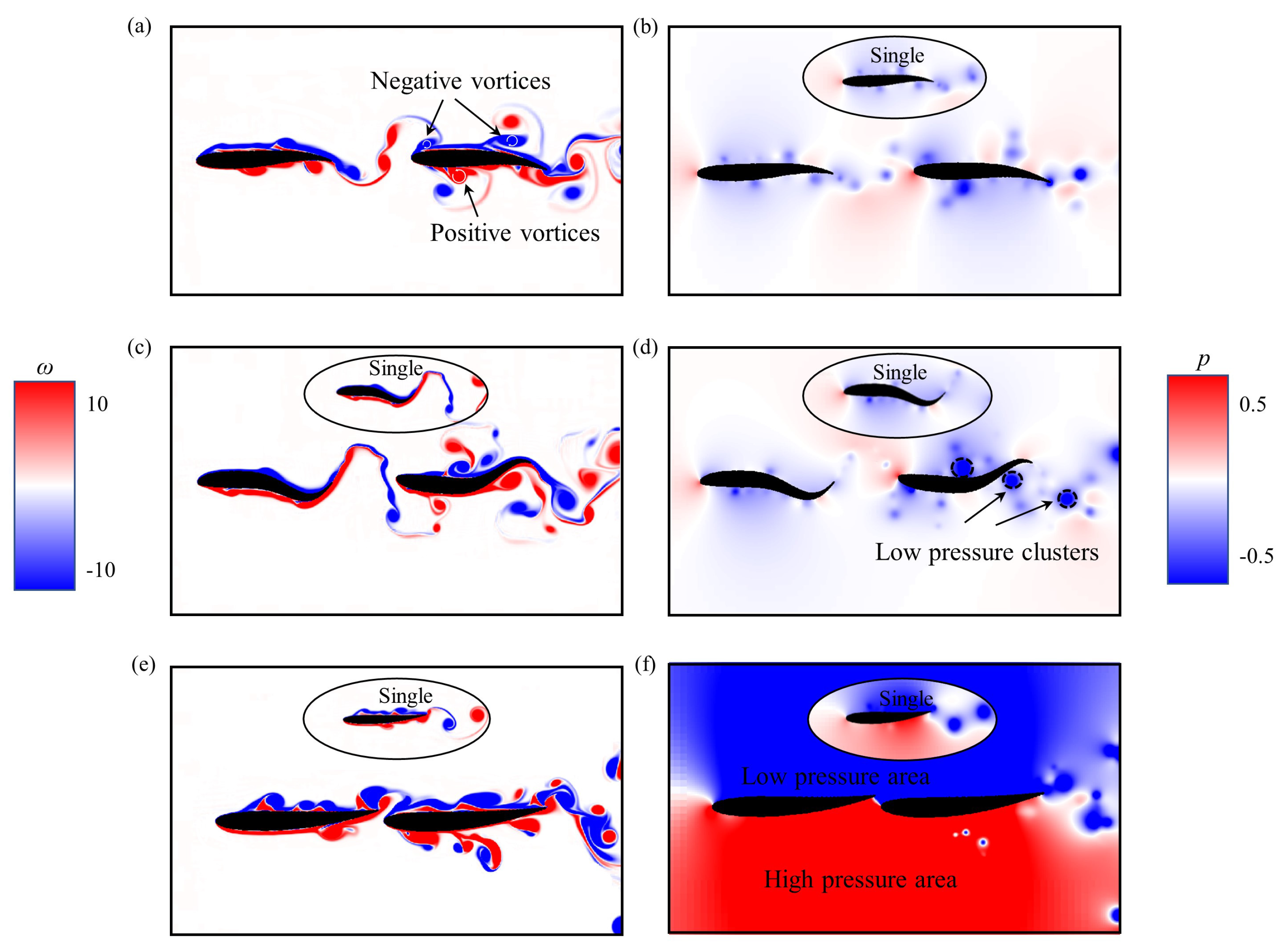
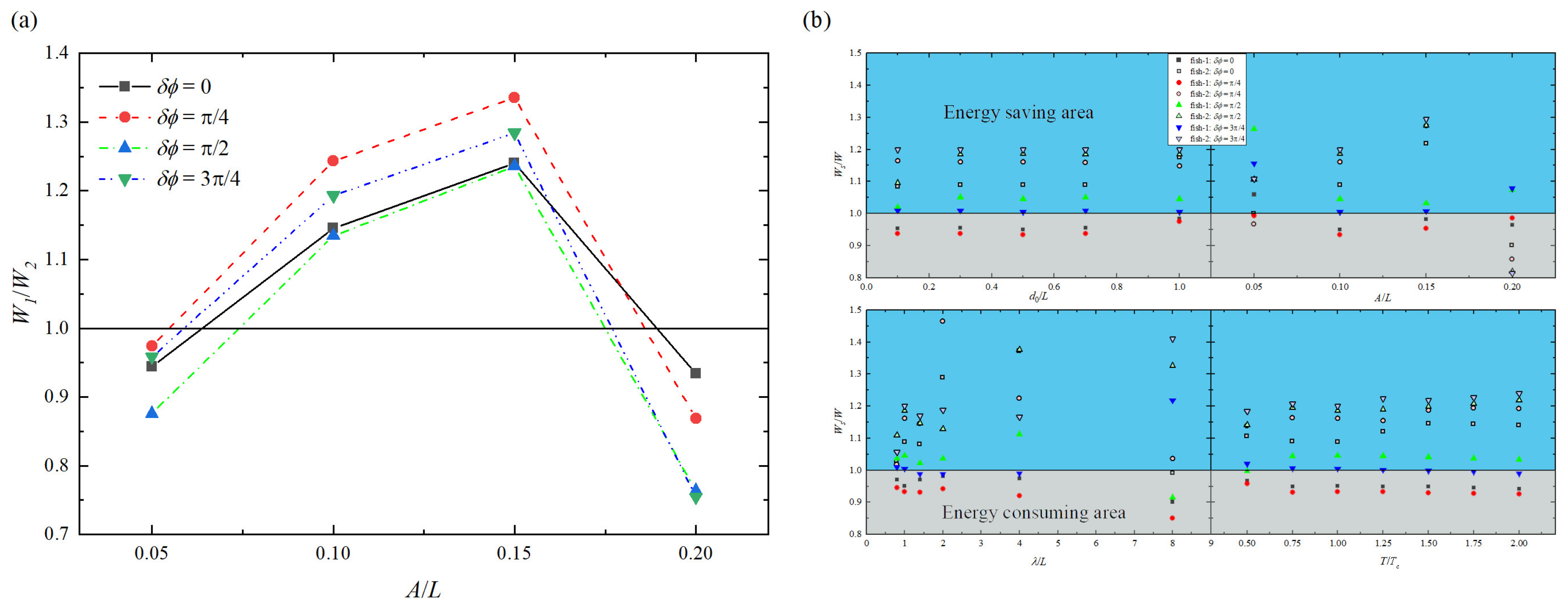
As shown in Figure 7a, when vortices shed by the upstream fish interact with the leading edge of the rear fish, they are split into positive vortices rotating anticlockwise and negative vortices rotating clockwise, and both parts interact with the shear layer around the fish body. The negative vortices move in the upper row and the positive vortices travel in the lower row, which allows the rear fish to benefit from the vortices shed by the upstream fish. Meanwhile, when 0.05L < A < 0.2L, the mean work done by the upstream fish is greater than that of the rear fish, as plotted in Figure 8a. This may explain why the rear fish is more energy-saving efficient than the upstream fish in most cases. On the other hand, due to the wake-splitting at the leading edges of the rear fish, the drag reduction of the upstream fish occurs [56], as shown in Figure 7c. At the same time, when the tail beat amplitude is either large or small, the mean work done by the rear fish is greater than that of the upstream fish, as plotted in Figure 8a. This may explain why the upstream fish is more energy-saving efficient than the rear fish in a few cases.
As shown in Figure 7d, there are multiple low pressure regions near the trailing edge of the rear fish, which allow the rear fish to receive the backward suction compared to the isolated fish. Meanwhile, the mean work done by rear fish is greater than that of the isolated fish under some situations, as given in Figure 8b. This may explain why the rear fish is higher energy consumption than the isolated fish in some cases.
From Figure 7a,c, it is observed that there is very little variation in the alignment or sizes of vortices just behind the upstream fish when the distance between two fish is moderate. These vortices experience negligible suction force produced by the rear fish, which is due to the smaller oscillation amplitude for leading edge of the rear fish. But when two fish are close to each other, as shown in Figure 7e, it can be seen that there is clear change in the alignment or sizes of vortices just behind the upstream fish. As a consequence, these vortices experience higher suction force produced by the rear fish. Meanwhile, the pressure difference around the two fish bodies is larger than that of the isolated fish, as given in Figure 7f. This is caused by the wake-splitting effect of the rear fish that generates the pressure enhancement. Moreover, in the case of A = 0.1L, = 8.0L, and = /4, the mean work done by upstream fish is greater than that of the isolated fish, as plotted in Figure 8b. This may explain why the upstream fish has higher energy consumption than the isolated fish in some cases. These results suggest that hydrodynamic interaction with a leader’s (upstream fish) wake can have both a beneficial and a detrimental impact on the performance of a follower (rear fish), which is consistent with the previous study by Novati et al. [63].
3.2. Scaling Laws for Re, St, and
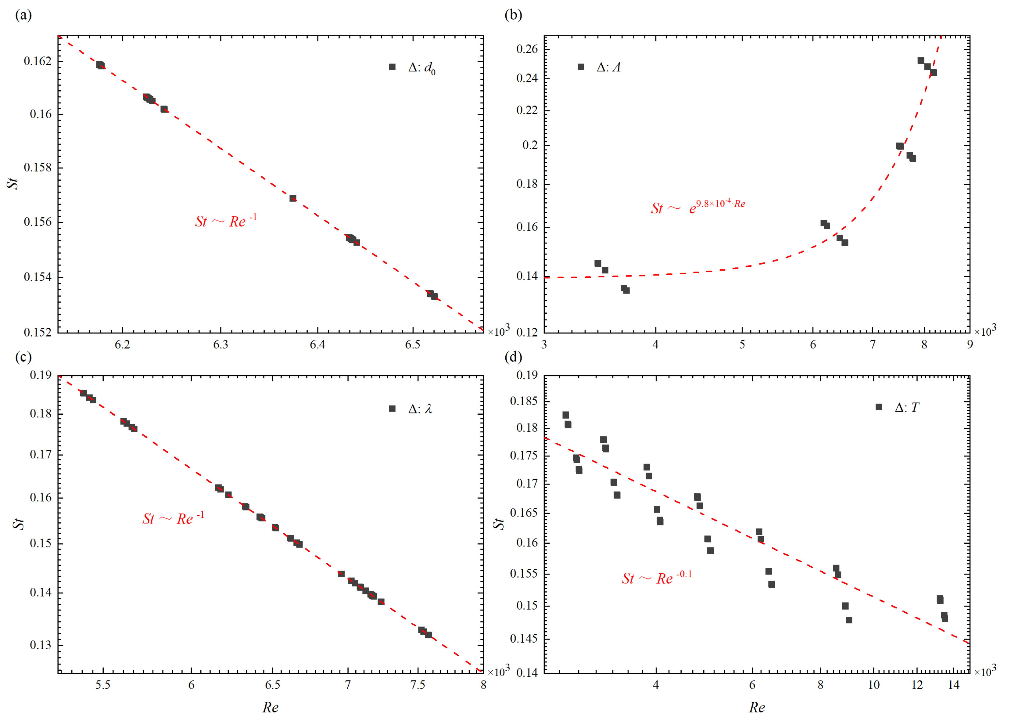
In this work, the mechanistic principle characterizing the locomotion of two tandem fish is revealed by deriving scaling laws related to the body kinematics (A, T, and ), arrangement of formation (), and fluid property (). In particular, when only changes, as shown in Figure 9a, the Strouhal number and the Reynolds number of two tandem fish can be scaled as
When only changes, the same scaling law for and Re can be obtained, as shown in Figure 9c. Similarly, when only T changes, as shown in Figure 9d, the power-law relationship of and Re is
From the results in Figure 9, it can be seen that the tail beat amplitude has great influence on the scaling law of and Re. It may be because a large tail swing causes a large disturbance in the flow field, which will make the shear layer around the fish body become extremely unstable (for example, see Figure 4c,d and Figure 7c).
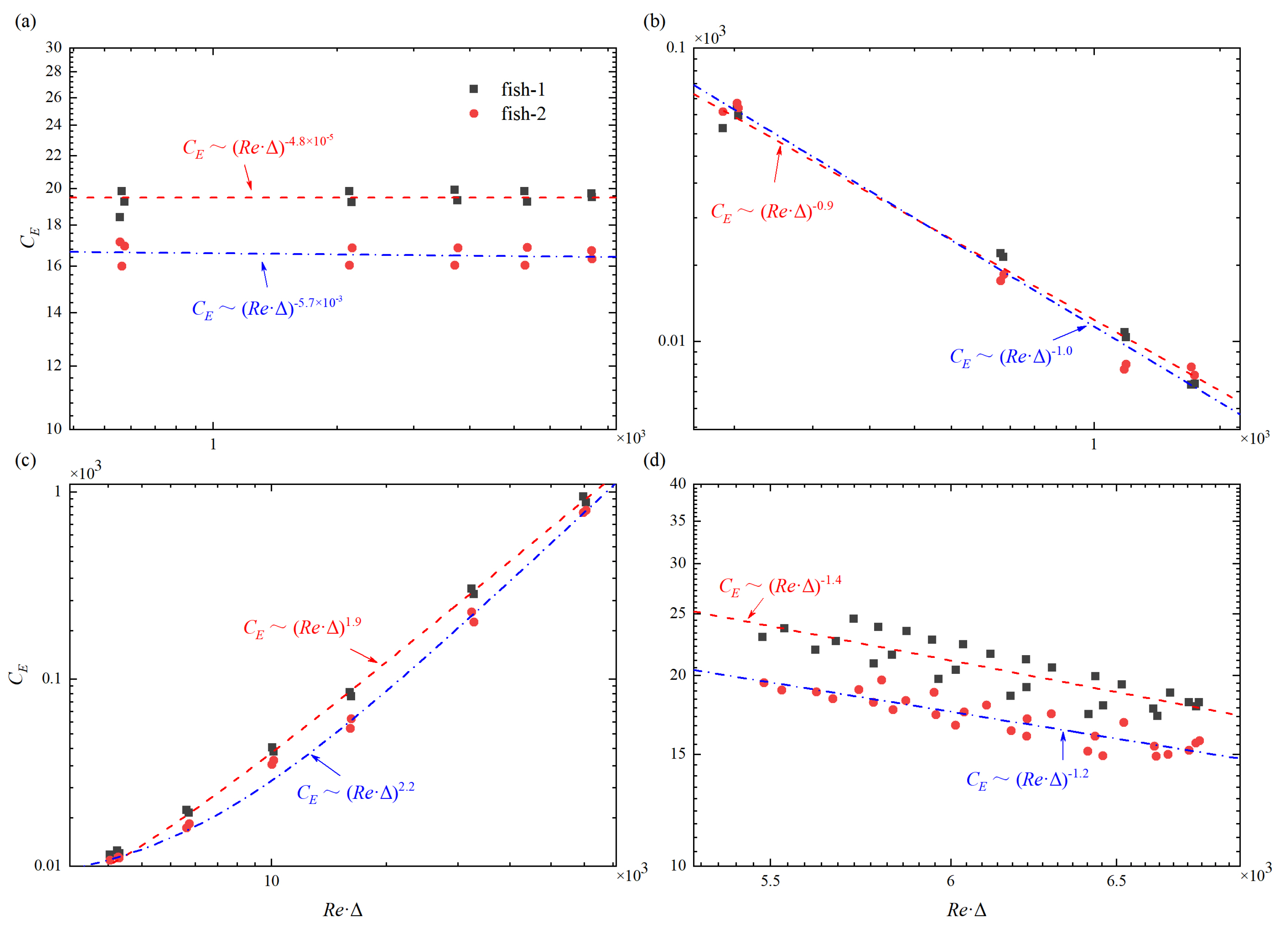
Despite the vast phylogenetic spread of inertial swimmers [64], it is found that their locomotory dynamics can be governed by the power law of ∼. Figure 10 shows different scaling laws between the upstream fish and the rear fish in a tandem arrangement. As shown in Figure 10a, when only changes, the scaling laws are
It is found that the energy consumption is hardly influenced by the Reynolds number. When only A changes, as shown in Figure 10b, the scaling laws are
It is noted that the scaling law of the upstream fish is almost the same as that of the rear fish. When only changes, as shown in Figure 10c, the scaling laws are
Unlike the scaling laws for and Re, the scaling laws for and Re show great difference between = and = . When only T changes, the scaling laws are
It can be observed that of the upstream fish is greater than that of the rear fish in most cases. This also can explain why the rear fish is more energy-saving-efficient than the upstream fish in most instances. In addition, it is clear that the index number “” of the upstream fish is always smaller than that of the rear fish. This means that the upstream fish is less influenced by the flow field as compared with the rear fish when they are in a tandem arrangement.
4. Conclusions
The effects of different swimming parameters on the hydrodynamic performance for two swimmers in the tandem formation in an initially quiescent flow are studied numerically in this paper. The conclusions are summarized as follows:
- In most cases, the swimming speed gain in the anti-phase swimming is smaller than that in other phases, and the speed gain shows a fixed trend under different phase differences. When the initial separation distance is larger, the speed gain is smaller. In addition, high swimming speed does not mean high speed gain.
- The rear fish is not always more energy-saving-efficient than the upstream fish. When the tail beat amplitude is either large or small, the energy consumption of the rear fish is higher than that of the upstream fish. Except for either large or small tail beat amplitude, the rear fish is more energy-saving-efficient than the upstream fish in most cases.
- Swimming in a tandem arrangement is not always more energy-saving-efficient than an isolated fish.
- The higher tail beat amplitude is the least friendly to the rear fish, while the lower tail beat amplitude is better for the upstream fish.
- For energy-saving efficiency, the optimal wavelength depends on the phase difference between two fish.
- There are scaling laws related to body kinematics (tail beat amplitude, period of oscillation, and wavelength), arrangement of formation (initial separation distance), and fluid property (kinematic viscosity).
The present investigations can provide a theoretical basis for the research of underwater vehicles and bionic robots. Nevertheless, there are still some limitations in this study. For example, the fish motion is controlled by a single degree of freedom with only longitudinal movement, which is different from the real fish swimming in nature. In our future work, more than one degree of freedom of fish motion will be considered to study the hydrodynamic characteristics of cluster swimming.
Supplementary Materials
The following supporting information can be downloaded at: https://0-www-mdpi-com.brum.beds.ac.uk/article/10.3390/fluids7060208/s1.
Author Contributions
Conceptualization, methodology, software, validation, visualization, and writing—original draft preparation: D.Y.; formal analysis, writing—review and editing, supervision, project administration, and funding acquisition: J.W. All authors have read and agreed to the published version of the manuscript.
Funding
This work has been supported by the National Natural Science Foundation of China grant No. 12072158 and the Natural Science Foundation of Jiangsu Province grant No. BK20191271. This work is also supported by the Priority Academic Program Development of Jiangsu Higher Education Institutions (PAPD).
Data Availability Statement
The data that support the findings of this study are available from the corresponding author upon reasonable request.
Conflicts of Interest
The authors declare no conflict of interest.
Abbreviations
The following abbreviations are used in this manuscript:
| Abbreviation | Value | Unit | Full Name |
| 1 × 10 | m/s | kinematic viscosity of fluid | |
| P | — | N·m/s | power of swimming |
| 1 × 10 | kg/m | fish body density | |
| V | 0.822 × 10 | m | fish body volume |
| — | m/s | constrained Lagrangian body velocity field | |
| — | N/m | constraint force density | |
| 1 × 10 | kg/m | fluid density | |
| f | 0.5-2 | s | tail beat frequency |
| — | s | angular frequency | |
| L | 0.1 | m | fish body length |
| 0.00026 | m | mesh size | |
| 0.0005 | s | time step | |
| m | 0.822 | kg | mass of fish |
| — | N | net force on the fish body in the x-direction | |
| — | N·m/s | mean net power spent | |
| — | N·m/s | mean lateral power spent | |
| u | — | m/s | forward swimming speed |
| — | m/s | mean swimming speed | |
| — | m/s | fluctuation of swimming speed | |
| — | N | cost and transport | |
| — | — | energy-consumption coefficient | |
| W | — | N·m | mean work done of fish swimming |
| 0.01–0.1 | m | initial separation distance | |
| A | 0.005–0.02 | m | tail beat amplitude |
| 0.08–0.8 | m | body wavelength | |
| T | 0.5–2.0 | s | period of oscillation |
| 1 | s | characteristic period of oscillation | |
| t | — | s | time |
| — | rad | phase difference | |
| 2897–13,513 | — | Reynolds number | |
| 0.13–0.25 | — | Strouhal number | |
| — | — | index of scaling law | |
| — | — | variable of swimming parameters | |
| — | — | power coefficient | |
| — | — | cell center of the grid | |
| — | — | position of a marker point |
References
- Weihs, D. Hydromechanics of fish schooling. Nature 1973, 241, 290–291. [Google Scholar] [CrossRef]
- Shaw, E. Schooling fishes. Am. Sci. 1978, 66, 166–175. [Google Scholar] [CrossRef]
- Pitcher, T.J.; Parrish, J.K. Functions of shoaling behavior in teleosts. In The Behaviour of Teleost Fishes; Springer: Boston, MA, USA, 1993; pp. 363–439. [Google Scholar]
- Godin, J.G.J.; Morgan, M.J. Predator avoidance and school size in a cyprinodontid fish, the banded killifish (Fundulus diaphanous lesueur). Behav. Ecol. Sociobiol. 1985, 16, 105–110. [Google Scholar] [CrossRef]
- Magurran, A.E.; Higham, A. Information transfer across fish shoals under predator threat. Ethology 1988, 78, 153–158. [Google Scholar] [CrossRef]
- Pitcher, T.J.; Magurran, A.E.; Winfield, I.J. Fish in larger shoals find food faster. Behav. Ecol. Sociobiol. 1982, 10, 149–151. [Google Scholar] [CrossRef]
- Fish, F.E. Energetics of swimming and flying in formation. Comments Theor. Biol. 1999, 5, 283–304. [Google Scholar]
- Killen, S.S.; Marras, S.; Steffensen, J.F.; McKenzie, D.J. Aerobic capacity influences the spatial position of individuals within fish schools. Biol. Sci. 2012, 279, 357–364. [Google Scholar] [CrossRef] [Green Version]
- Hemelrijk, C.K.; Reid, D.A.P.; Hildenbrandt, H.; Padding, J.T. The increased efficiency of fish swimming in a school. Fish Fish. 2015, 16, 511–521. [Google Scholar] [CrossRef] [Green Version]
- Chao, L.; Pan, G.; Zhang, D.; Yan, G. On the two staggered swimming fish. Chaos Solitons Fractals 2019, 129, 260–262. [Google Scholar] [CrossRef]
- Park, S.; Sung, H. Hydrodynamics of flexible fins propelled in tandem, diagonal, triangular and diamond configurations. J. Fluid Mech. 2018, 840, 154–189. [Google Scholar] [CrossRef]
- Deng, J.; Shao, X.; Yu, Z. Hydrodynamic Studies on Two Traveling Wavy Foils in Tandem Arrangement. Phys. Fluids 2007, 19, 113104. [Google Scholar] [CrossRef]
- Kang, L.; Peng, Z.; Huang, H.; Lu, X.; Cui, W. Active external control effect on the collective locomotion of two tandem self-propelled flapping plates. Phys. Fluids 2021, 33, 101901. [Google Scholar] [CrossRef]
- Novati, G.; Verma, S.; Alexeev, D.; Rossinelli, D.; van Rees, W.M.; Koumoutsakos, P. Synchronisation through learning for two self-propelled swimmers. Bioinspir. Biomimetics 2017, 12, 036001. [Google Scholar] [CrossRef] [PubMed] [Green Version]
- Lin, X.; Wu, J.; Zhang, T.; Yang, L. Flow-mediated organization of two freely flapping swimmers. J. Fluid Mech. 2021, 912, A37. [Google Scholar] [CrossRef]
- Lin, X.; Wu, J.; Zhang, T.; Yang, L. Self-organization of multiple self-propelling flapping foils: Energy saving and increased speed. J. Fluid Mech. 2020, 884, R1. [Google Scholar] [CrossRef]
- Lin, X.; Wu, J.; Yang, L.; Dong, H. Two-dimensional hydrodynamic schooling of two flapping swimmers initially in tandem formation. J. Fluid Mech. 2022, 941, A29. [Google Scholar] [CrossRef]
- Herskin, J.; Steffensen, J.F. Energy savings in sea bass swimming in a school: Measurements of tail beat frequency and oxygen consumption at different swimming speeds. J. Fish Biol. 1998, 53, 366–376. [Google Scholar] [CrossRef]
- Marras, S.; Killen, S.S.; Lindstrom, J.; Mckenzie, D.J.; Steffensen, J.F.; Domenici, P. Fish swimming in schools save energy regardless of their spatial position. Behav. Ecol. Sociobiol. 2015, 69, 219–226. [Google Scholar] [CrossRef] [Green Version]
- Svendsen, J.C.; Skov, J.; Bildsoe, M.; Steffensen, J.F. Intra-school positional preference and reduced tail beat frequency in trailing positions in schooling roach under experimental conditions. J. Fish Biol. 2003, 32, 834–846. [Google Scholar] [CrossRef] [Green Version]
- Bhalla, A.P.S.; Rahul, B.; Griffith, B.E.; Neelesh, A.P. A unified mathematical framework and an adaptive numerical method for fluid–structure interaction with rigid, deforming, and elastic bodies. J. Comput. Phys. 2013, 250, 446–476. [Google Scholar] [CrossRef]
- Griffith, B.E.; Hornung, D.; McQueen, D.M.; Peskin, C.S. An adaptive, formally second order accurate version of the immersed boundary method. J. Comput. Phys. 2007, 223, 10–49. [Google Scholar] [CrossRef]
- Zhao, H.; Freund, J.B.; Moser, R.D. A fixed-mesh method for incompressible flow-structure systems with finite solid deformations. J. Comput. Phys. 2008, 227, 3114–3140. [Google Scholar] [CrossRef]
- Herschlag, G.; Miller, L. Reynolds number limits for jet propulsion: A numerical study of simplified jellyfish. J. Theor. Biol. 2011, 285, 84–95. [Google Scholar] [CrossRef] [Green Version]
- Tytell, E.D.; Hsu, C.Y.; Williams, T.L.; Cohen, A.H.; Fauci, L.J. Interactions between internal forces, body stiffness, and fluid environment in a neuromechanical model of lamprey swimming. Proc. Natl. Acad. Sci. USA 2010, 107, 19832–19837. [Google Scholar] [CrossRef] [PubMed] [Green Version]
- Wang, L.; Wu, C. An adaptive version of ghost-cell immersed boundary method for incompressible flows with complex stationary and moving boundaries. Sci. China Phys. Mech. Astron. 2010, 53, 923–932. [Google Scholar] [CrossRef]
- Borazjani, I.; Sotiropoulos, F. On the role of form and kinematics on the hydrodynamics of self-propelled body/caudal fin swimming. J. Exp. Biol. 2010, 213, 89–107. [Google Scholar] [CrossRef] [Green Version]
- Tytell, E.D.; Lauder, G.V. The hydrodynamics of eel swimming. I: Wake structure. J. Exp. Biol. 2004, 207, 1825–1841. [Google Scholar] [CrossRef] [Green Version]
- Videler, J.J.; Hess, F. Fast continuous swimming of two pelagic predators, saithe (Pollachius virens) and mackerel (Scomber scombrus): A kinematic analysis. J. Exp. Biol. 1984, 109, 209–228. [Google Scholar] [CrossRef]
- Pedley, T.J.; Hill, S.J. Large-amplitude undulatory fish swimming: Fluid mechanics coupled to internal mechanics. J. Exp. Biol. 1999, 202, 3431–3438. [Google Scholar] [CrossRef]
- Tytell, E.D. Do trout swim better than eels? Challeges for estimating performance based on the wake of self-propelled bodies. Exp. Fluids. 2007, 43, 701–712. [Google Scholar] [CrossRef]
- Bale, R.; Hao, M.; Bhalla, A.P.S.; Patankar, N.A. Energy efficiency and allometry of movement of swimming and flying animals. Proc. Natl Acad. Sci. USA 2014, 111, 7517–7521. [Google Scholar] [CrossRef] [PubMed] [Green Version]
- Griffith, B.E.; Bhalla, A.P.S. IBAMR: An Adaptive and Distributed-memory Parallel Implementation of the Immersed Boundary Method. Available online: https://ibamr.github.io/ (accessed on 9 August 2020).
- Lauder, G.V. Function of the caudal fin during locomotion in fishes: Kinematics, flow visualization, and evolutionary patterns. Am. Zool. 2000, 40, 101–122. [Google Scholar] [CrossRef] [Green Version]
- Lauder, G.V.; Nauen, J.C.; Drucker, E.G. Experimental hydrodynamics and evolution: Function of median fins in ray-finned fishes. Integr. Comput. Biol. 2002, 42, 1009–1017. [Google Scholar] [CrossRef] [PubMed] [Green Version]
- Dabiri, J.O.; Gharib, M. Sensitivity analysis of kinematic approximations in dynamic medusan swimming models. J. Exp. Biol. 2003, 206, 3675–3680. [Google Scholar] [CrossRef] [PubMed] [Green Version]
- Curet, O.M.; Patankar, N.A.; Lauder, G.V.; MacIver, M.A. Aquatic manoeuvering with counter-propagating waves: A novel locomotive strategy. J. R. Soc. Interface 2011, 8, 1041–1050. [Google Scholar] [CrossRef] [Green Version]
- Curet, O.M.; Patankar, N.A.; Lauder, G.V.; MacIver, M.A. Mechanical properties of a bio-inspired robotic knifefish with an undulatory propulsor. Bioinspir. Biomimetics 2011, 6, 026004. [Google Scholar] [CrossRef] [Green Version]
- Ruiz-Torres, R.; Curet, O.M.; Lauder, G.V.; MacIver, M.A. Kinematics of the ribbon fin in hovering and swimming of the electric ghost knifefish. J. Exp. Biol. 2013, 216, 823–834. [Google Scholar]
- Nangia, N.; Johansen, H.; Patankar, N.A.; Bhalla, A.P.S. A moving control volume approach to computing hydrodynamic forces and torques on immersed bodies. J. Comput. Phys. 2017, 347, 437–462. [Google Scholar] [CrossRef] [Green Version]
- Hornung, R.D.; Kohn, S.R. Managing application complexity in the SAMRAI object-oriented framework. Concurr. Comput. 2002, 14, 347–368. [Google Scholar] [CrossRef]
- Hornung, R.D.; Wissink, A.M.; Kohn, S.R. Managing complex data and geometry in parallel structured AMR applications. Eng. Comput. 2006, 22, 181–195. [Google Scholar] [CrossRef]
- SAMRAI: Structured Adaptive Mesh Refinement Application Infrastructure. Available online: http://www.llnl.gov/CASC/SAMRAI (accessed on 9 August 2020).
- Berger, M.J.; Rigoutsos, I. An algorithm for point clustering and grid generation. IEEE. Trans. Syst. Man. Cybern. 1991, 21, 1278–1286. [Google Scholar] [CrossRef]
- Griffith, B.E. An accurate and efficient method for the incompressible Navier-Stokes equations using the projection method as a preconditioner. J. Comput. Phys. 2009, 228, 7565–7595. [Google Scholar] [CrossRef]
- Griffith, B.E.; Patankar, N.A. Immersed methods for fluid-structure interaction. Annu. Rev. Fluid Mech. 2020, 52, 421–448. [Google Scholar] [CrossRef] [PubMed] [Green Version]
- Balay, S.; Buschelman, K.; Gropp, W.D.; Kaushik, D.; Knepley, M.G.; McInnes, L.C.; Smith, B.F.; Zhang, H. PETSc Web Page 2009. Available online: http://www.mcs.anl.gov/petsc (accessed on 9 August 2020).
- Bale, R.; Bhalla, A.P.S.; Neveln, I.D.; MacIver, M.A.; Patankar, N.A. Convergent evolution of mechanically optimal locomotion in aquatic invertebrates and vertebrates. PLoS Biol. 2015, 13, 1002123. [Google Scholar] [CrossRef] [Green Version]
- Bhalla, A.P.S.; Griffith, B.E.; Patankar, N.A. A forced damped oscillation framework for undulatory swimming provides new insights into how propulsion arises in active and passive swimming. PLoS Comput. Biol. 2013, 9, 100309. [Google Scholar] [CrossRef] [Green Version]
- Dombrowski, T.; Jones, S.K.; Bhalla, A.P.S.; Katsikis, G.; Griffith, B.E.; Klotsa, D. Transition in swimming direction in a model self-propelled inertial swimmer. Phys. Rev. Fluid 2019, 4, 021101. [Google Scholar] [CrossRef]
- Hoover, A.P.; Tytell, E. Decoding the Relationships between Body Shape, Tail Beat Frequency, and Stability for Swimming Fish. Fluids 2020, 5, 215. [Google Scholar] [CrossRef]
- Patel, N.K.; Bhalla, A.P.S.; Patankar, N.A. A new constraint-based formulation for hydrodynamically resolved computational neuromechanics of swimming animals. J. Comput. Phys. 2018, 375, 684–716. [Google Scholar] [CrossRef]
- Voesenk, C.J.; Li, G.; Muijres, F.T.; van Leeuwen, J.L. Experimental–numerical method for calculating bending moments in swimming fish shows that fish larvae control undulatory swimming with simple actuation. PLoS Biol. 2020, 18, 3000462. [Google Scholar] [CrossRef]
- Zhang, D.; Pan, G.; Chao, L.; Zhang, Y. Effects of Reynolds number and thickness on an undulatory self-propelled foil. Phys. Fluids 2018, 30, 071902. [Google Scholar] [CrossRef]
- Nangia, N.; Patankar, N.A.; Bhalla, A.P.S. A DLM immersed boundary method based wave-structure interaction solver for high density ratio multiphase flows. J. Comput. Phys. 2019, 398, 108804. [Google Scholar] [CrossRef] [Green Version]
- Khalid, M.; Imran, A.; Dong, H. Hydrodynamics of a Tandem Fish School with Asynchronous Undulation of Individuals. J. Fluids Struc. 2016, 66, 19–35. [Google Scholar] [CrossRef] [Green Version]
- Diana, R.G.; Aider, J.L.; Wesfreid, J.E. Transitions in the wake of a flapping foil. Phys. Rev. E 2008, 77, 016308. [Google Scholar] [CrossRef] [PubMed] [Green Version]
- Schnipper, T.; Andersen, A.; Bohr, T. Vortex wakes of a flapping foil. J. Fluid Mech. 2009, 633, 411–423. [Google Scholar] [CrossRef] [Green Version]
- Williamson, C.H.K.; Roshko, A. Vortex formation in the wake of an oscillating cylinder. J. Fluids Struc. 1988, 2, 355–381. [Google Scholar] [CrossRef]
- Han, P.; Pan, Y.; Liu, G.; Dong, H. Propulsive performance and vortex wakes of multiple tandem foils pitching in-line. J. Fluids Struc. 2022, 108, 103422. [Google Scholar] [CrossRef]
- Ramananarivo, S.; Fang, F.; Oza, A.; Zhang, J.; Ristroph, L. Flow interactions lead to orderly formations of flapping wings in forward flight. Phys. Rev. Fluids 2016, 1, 071201. [Google Scholar] [CrossRef]
- Williams, T.M.; Friedl, W.A.; Haun, J. Balancing power and speed in bottlenose dolphins (Tursiops truncatus). Symp. Zool. Soc. Lond. 1993, 66, 383–394. [Google Scholar]
- Novati, G.; Verma, S.; Alexeev, D.; Rossinelli, D.; van Rees, W.M.; Koumoutsakos, P. Synchronised Swimming of Two Fish. arXiv 2016, arXiv:1610.04248. [Google Scholar]
- Gazzola, M.; Argentina, M.; Mahadevan, L. Scaling macroscopic aquatic locomotion. Nat. Phys. 2014, 10, 758–761. [Google Scholar] [CrossRef] [Green Version]
Figure 1.
(a) Sketch of computational domain. (b) Fish parameters.

Figure 2.
(a) Lagrange points marking structure and adaptive mesh sketch. (b) Numerical discretization of the Lagrangian markers (■, orange). (c) A single Cartesian grid cell on which the components of the velocity field are approximated on the cell faces (⟶, black), and the Lagrangian quantities are approximated on the marker point (■, orange), which can be arbitrarily placed on the Eulerian grid.

Figure 3.
Mean swimming speeds with different (a) initial separation distance , (b) tail beat amplitude A, (c) wave length , and (d) period of oscillation T.
Figure 3.
Mean swimming speeds with different (a) initial separation distance , (b) tail beat amplitude A, (c) wave length , and (d) period of oscillation T.

Figure 4.
Instantaneous vorticity contours of two self-propelled fish in the tandem arrangement at swimming parameters (a) = 0.1L, A = 0.1L, = /2, (b) = 0.1L, A = 0.1L, = 3/4, (c) = 0.5L, A = 0.2L, = /2, and (d) = 0.5L, A = 0.2L, = /4. Other parameters are the same: T = 1.0 and = 1.0L.
Figure 4.
Instantaneous vorticity contours of two self-propelled fish in the tandem arrangement at swimming parameters (a) = 0.1L, A = 0.1L, = /2, (b) = 0.1L, A = 0.1L, = 3/4, (c) = 0.5L, A = 0.2L, = /2, and (d) = 0.5L, A = 0.2L, = /4. Other parameters are the same: T = 1.0 and = 1.0L.

Figure 5.
Time histories of swimming speed and power coefficient. (a,b) = 0.1L, A = 0.1L, and (c,d) = 0.5L, A = 0.2L. Other parameters are the same: T = 1.0, = 1.0L and = /2.
Figure 5.
Time histories of swimming speed and power coefficient. (a,b) = 0.1L, A = 0.1L, and (c,d) = 0.5L, A = 0.2L. Other parameters are the same: T = 1.0, = 1.0L and = /2.

Figure 6.
Ratios of cost of transport with different (a) initial separation distance , (b) tail beat amplitude A, (c) wave length , and (d) period of oscillation T. in the denominator represents either of the upstream fish or of the rear fish.
Figure 6.
Ratios of cost of transport with different (a) initial separation distance , (b) tail beat amplitude A, (c) wave length , and (d) period of oscillation T. in the denominator represents either of the upstream fish or of the rear fish.

Figure 7.
Instantaneous vorticity contours and pressure contours of two self-propelled fish in the tandem formation at swimming parameters (a,b) A = 0.1L, = 2.0L, = /4, (c,d) A = 0.2L, = 1.0L, = 3/4, and (e,f) A = 0.1L, = 8.0L, = /4. Other parameters are the same: T = 1.0 and = 0.5L.
Figure 7.
Instantaneous vorticity contours and pressure contours of two self-propelled fish in the tandem formation at swimming parameters (a,b) A = 0.1L, = 2.0L, = /4, (c,d) A = 0.2L, = 1.0L, = 3/4, and (e,f) A = 0.1L, = 8.0L, = /4. Other parameters are the same: T = 1.0 and = 0.5L.

Figure 8.
Ratios of mean work done by (a) upstream fish to rear fish and (b) isolated fish to two fish in a tandem arrangement with different swimming parameters: (top left), A (top right), (bottom left), and T (bottom right), where the W in the denominator represents the of the upstream fish and the of the rear fish, respectively. The blue block represents the energy saving-area and the gray block represents the energy-consuming area.

Figure 9.
The Reynolds number in different (a) initial separation distance , (b) tail beat amplitude A, (c) wave length , and (d) period of oscillation T as a function of the Strouhal number. The red dash-dot line in panel represents the scaling law for the Reynolds number and the Strouhal number, where “” represents the swimming parameters variables.

Figure 10.
The energy consumption coefficient varies as a function of the Reynolds number and different change of (a) initial separation distance ( = ), (b) tail beat amplitude ( = A), (c) wave length ( = ), and (d) period of oscillation ( = T).
Figure 10.
The energy consumption coefficient varies as a function of the Reynolds number and different change of (a) initial separation distance ( = ), (b) tail beat amplitude ( = A), (c) wave length ( = ), and (d) period of oscillation ( = T).


Table 1.
The overview of speed gains with all studied parameters.
| (( − )/) × 100% | |||||
|---|---|---|---|---|---|
| 0 | /4 | /2 | 3/4 | ||
| d0 | 0.10L | 6.8% | 5.4% | 4.4% | 2.0% |
| 0.30L | 6.8% | 5.4% | 1.2% | 2.0% | |
| 0.50L | 6.8% | 5.4% | 1.2% | 2.0% | |
| 0.70L | 6.8% | 5.4% | 1.2% | 2.0% | |
| 1.00L | 2.3% | 2.1% | 1.2% | 2.0% | |
| A | 0.05L | 19.5% | 18.7% | 11.0% | 13.1% |
| 0.10L | 6.8% | 5.4% | 1.2% | 2.0% | |
| 0.15L | 4.4% | 3.5% | 0.8% | 1.1% | |
| 0.20L | 3.1% | 1.4% | 4.7% | 4.9% | |
| 0.80L | 7.3% | 6.2% | 2.2% | 3.1% | |
| 1.00L | 6.8% | 5.4% | 1.2% | 2.0% | |
| 1.40L | 5.4% | 4.7% | 1.4% | 2.4% | |
| 2.00L | 8.4% | 7.6% | 0.8% | 1.9% | |
| 4.00L | 9.9% | 8.7% | 1.5% | 2.4% | |
| 8.00L | 8.8% | 7.2% | 4.4% | 13.1% | |
| T | 0.50 | 2.9% | 2.5% | 0.8% | 0.9% |
| 0.75 | 6.6% | 5.2% | 1.1% | 1.8% | |
| 1.00 | 6.8% | 5.4% | 1.2% | 2.0% | |
| 1.25 | 7.0% | 5.7% | 1.3% | 2.2% | |
| 1.50 | 7.4% | 5.9% | 1.5% | 2.4% | |
| 1.75 | 7.5% | 6.2% | 1.6% | 2.6% | |
| 2.00 | 7.7% | 6.4% | 1.8% | 2.8% | |
Table 2.
The overview of energy-saving efficiency with all studied parameters.
| (( − )/) × 100% | ||||||
|---|---|---|---|---|---|---|
| 0 | /4 | /2 | 3/4 | |||
| d0 | 0.10L | fish-1 | 1.9% | −1.1% | 6.1% | 2.9% |
| fish-2 | 13.7% | 18.3% | 12.5% | 1832% | ||
| 0.30L | fish-1 | 2.0% | −1.1% | 6.0% | 2.9% | |
| fish-2 | 14.1% | 18.3% | 16.7% | 18.3% | ||
| 0.50L | fish-1 | 1.5% | −1.6% | 5.5% | 2.5% | |
| fish-2 | 14.1% | 18.3% | 16.7% | 18.3% | ||
| 0.70L | fish-1 | 1.9% | −1.1% | 6.0% | 2.9% | |
| fish-2 | 14.0% | 18.3% | 16.7% | 18.3% | ||
| 1.00L | fish-1 | 0.6% | −0.5% | 5.5% | 2.5% | |
| fish-2 | 16.8% | 14.7% | 16.7% | 18.3% | ||
| A | 0.05L | fish-1 | 21.0% | 15.1% | 28.7% | 23.5% |
| fish-2 | 16.3% | 12.9% | 18.6% | 20.2% | ||
| 0.10L | fish-1 | 1.5% | −1.6% | 5.5% | 2.5% | |
| fish-2 | 14.1% | 18.3% | 16.7% | 18.3% | ||
| 0.15L | fish-1 | 2.5% | −1.2% | 3.9% | 1.8% | |
| fish-2 | 21.2% | 24.2% | 22.2% | 23.5% | ||
| 0.20L | fish-1 | −0.6% | 0.1% | 11.1% | 11.7% | |
| fish-2 | −7.7% | −15.0% | −16.5% | −17.2% | ||
| 0.80L | fish-1 | 4.0% | 0.5% | 5.5% | 3.9% | |
| fish-2 | 9.1% | 7.8% | 11.6% | 7.9% | ||
| 1.00L | fish-1 | 1.5% | −1.6% | 5.5% | 2.5% | |
| fish-2 | 14.1% | 18.3% | 16.7% | 18.3% | ||
| 1.40L | fish-1 | 2.3% | −2.7% | 3.5% | 1.1% | |
| fish-2 | 12.2% | 16.4% | 14.0% | 16.5% | ||
| 2.00L | fish-1 | 5.9% | 1.3% | 4.3% | 0.7% | |
| fish-2 | 28.4% | 36.7% | 12.0% | 17.4% | ||
| 4.00L | fish-1 | 6.6% | 0.1% | 11.5% | 1.4% | |
| fish-2 | 33.8% | 25.0% | 28.5% | 16.1% | ||
| 8.00L | fish-1 | −2.0% | −9.7% | 21.4% | 3.4% | |
| fish-2 | 7.4% | 10.1% | 32.1% | 33.3% | ||
| T | 0.50 | fish-1 | −0.4% | −1.8% | 0.5% | 3.0% |
| fish-2 | 12.1% | 14.3% | 13.1% | 16.3% | ||
| 0.75 | fish-1 | 1.3% | −2.2% | 5.3% | 2.4% | |
| fish-2 | 14.0% | 18.2% | 17.2% | 18.7% | ||
| 1.00 | fish-1 | 1.5% | −1.6% | 5.5% | 2.5% | |
| fish-2 | 14.1% | 18.3% | 16.7% | 18.3% | ||
| 1.25 | fish-1 | 1.5% | −1.5% | 5.5% | 2.3% | |
| fish-2 | 16.6% | 18.1% | 16.9% | 20.0% | ||
| 1.50 | fish-1 | 1.9% | −1.6% | 5.3% | 2.3% | |
| fish-2 | 18.6% | 20.6% | 17.7% | 19.8% | ||
| 1.75 | fish-1 | 1.6% | −1.5% | 5.2% | 2.1% | |
| fish-2 | 18.7% | 21.1% | 18.5% | 20.5% | ||
| 2.00 | fish-1 | 1.4% | −1.6% | 5.0% | 1.9% | |
| fish-2 | 18.7% | 21.4% | 19.4% | 21.6% | ||
Publisher’s Note: MDPI stays neutral with regard to jurisdictional claims in published maps and institutional affiliations. |
© 2022 by the authors. Licensee MDPI, Basel, Switzerland. This article is an open access article distributed under the terms and conditions of the Creative Commons Attribution (CC BY) license (https://creativecommons.org/licenses/by/4.0/).
Share and Cite
MDPI and ACS Style
Yang, D.; Wu, J. Hydrodynamic Interaction of Two Self-Propelled Fish Swimming in a Tandem Arrangement. Fluids 2022, 7, 208. https://0-doi-org.brum.beds.ac.uk/10.3390/fluids7060208
AMA Style
Yang D, Wu J. Hydrodynamic Interaction of Two Self-Propelled Fish Swimming in a Tandem Arrangement. Fluids. 2022; 7(6):208. https://0-doi-org.brum.beds.ac.uk/10.3390/fluids7060208
Chicago/Turabian StyleYang, Dewu, and Jie Wu. 2022. "Hydrodynamic Interaction of Two Self-Propelled Fish Swimming in a Tandem Arrangement" Fluids 7, no. 6: 208. https://0-doi-org.brum.beds.ac.uk/10.3390/fluids7060208