
Magnetohydrodynamics Solver for a Two-Phase Free Surface Flow Developed in OpenFOAM


1
General Fusion Inc., Burnaby, BC V3N 4T5, Canada
2
School of Engineering and Materials Science, Queen Mary University of London, London E1 4NS, UK
*
Author to whom correspondence should be addressed.
†
These authors contributed equally to this work.
Fluids 2022, 7(7), 210; https://0-doi-org.brum.beds.ac.uk/10.3390/fluids7070210
Submission received: 25 April 2022
/
Revised: 12 June 2022
/
Accepted: 15 June 2022
/
Published: 21 June 2022
(This article belongs to the Special Issue The Recent Advances in Magnetorheological Fluids)
Abstract
:A magnetohydrodynamics solver (“mhdCompressibleInterFoam”) has been developed for a compressible two-phase flow with a free surface by extending “compressibleInterFoam” solver within OpenFOAM suite. The primary goal is to develop a tool to simulate compression of magnetic fields in vacuum and simplified magnetized plasma targets by imploding rotating liquid metal liners in the context of a Magnetized Target Fusion (MTF) concept in pursuit by General Fusion Inc. At present, the solver is limited to axisymmetric problems and the magnetic field evolution is solved in terms of toroidal field component and poloidal flux functions. The solver has been validated and verified using a number of test cases for which analytical or other numerical solutions are provided. Those tests cases include: (i) compression of toroidal and poloidal magnetic fields in vacuum and cylindrical geometry, (ii) axisymmetric annular Hartmann flow, and (iii) compression of magnetized target initialized with a Grad–Shafranov equilibrium state in a cylindrical geometry. A methodology to incorporate conductive solid regions into simulation has also been developed. Capability of the code is demonstrated by simulating a complex case of compressing a magnetized target, which is injected during implosion of a rotating liquid metal liner with an initially soaked poloidal magnetic field. An application of the solver to simulate compression of a magnetized target in a geometry and parameters relevant to the Fusion Demonstration Plant (FDP) being developed by General Fusion Inc. is also demonstrated.
1. Introduction
Development of an MHD solver capable of handling compressible fluids with a free-surface has been prompted by simulation needs in General Fusion Inc. to advance development of the Fusion Demonstration Plant (FDP) [1]. The magnetized Target Fusion (MTF) scheme in pursuit by General Fusion Inc. relies on achieving nuclear fusion conditions during compression of magnetized plasma by imploding rotating liquid metal liner [1]. A schematic of the system is shown in Figure 1. Magnetized plasma is injected into a vacuum cavity inside a rotating liquid metal liner. Pistons, driven by high pressure gas, push on the outer surface of the rotating metal liner causing it to implode and compress a magnetized plasma target. In the vertical direction, the pistons are arranged into layers, and the trajectory of pistons can be varied from layer to layer. This allows to shape the liner as it implodes, starting up from a cylindrical one and ending up with more like a spherical one during the implosion. Simulating the entire system is challenging, as it requires combining the dynamics of magnetized plasma, the dynamics of the imploding liquid metal liner, and, to some extent, of the piston system. One of the main issues in simulating plasma and liner dynamics simultaneously is that they operate at different times scales; plasma simulations usually require a much smaller time step (in the order of ) compared with the hydrodynamics of the liner (in the order of ).
A great amount of work has been performed by simulating plasma evolution and hydrodynamics of liner implosion independently. Plasma evolution during formation and its stability during compression has been studied by dedicated plasma codes such as Versatile Advection Code (VAC) [2], NIMROD [3] and CORSICA [4] and DCON [5], whereas the shape and trajectory of the imploding liner have been provided as an input. Dynamics and stability of the rotating imploding liquid metal liner has been extensively simulated using the hydrodynamic “compressibleInterFoam” solver, which is part of the open source C++ libraries of OpenFOAM [6]. Simulating plasma evolution and liner hydrodynamics separately has its limitations, as some degree of coupling between magnetized plasma and liquid metal liner is expected during compression. This coupling is case dependent and it is difficult to predict in prior how significant it is in order to reliably simulate compression process. Current research focuses on investigating how significant the effect of magnetic field is on the liner dynamics during implosion. As the vacuum magnetic field (or magnetic target) gets compressed, the shape and trajectory of the liner may be affected by: (i) diffusion of magnetic field into the liner and the surrounding electrically conductive structure and (ii) the magnetic pressure pushing back from the compressed magnetic field. The effect of the magnetic field on the evolution of surface perturbations at the inner liner surface during implosion can be also studied by the including MHD effects into the simulations. More complex issues of how, for example, the stability of the plasma is affected by interaction of the magnetic field with the liquid metal liner is out of scope for this study.
Several concurrent approaches have been persuaded in General Fusion to achieve coupling between the magnetic field/plasma evolution and the liquid metal liner implosion dynamics. One of them is to simulate the plasma and liquid liner by separately dedicated codes and couple at the interface, i.e., VAC-OF coupling [7]. Another one, is to simulate the liner dynamics with a hydro code and then add part of the liner (along with velocity field) as an additional layer surrounding the plasma domain in the VAC plasma code [2]. With this approach, it is assumed that the liner trajectory is not affected by the plasma evolution, but the diffusion of the magnetic field into the liner is captured during compression.
The current approach is to extend the multiphase hydrodynamic solver, which we extensively use to simulate imploding liquid liner dynamics (“compressibleInterFoam” within OpenFOAM) to include the evolution of the magnetic fields, i.e., to obtain a two-phase MHD solver. “compressibleInterFoam” is a multiphase solver which uses VOF (Volume of Fluid) phase-fraction-based interface-capturing approach and is suitable for modeling two compressible immiscible fluids [8]. It has been successfully used in General Fusion to simulate imploding liners dynamics and study interface instabilities and means of their suppression [9,10,11]. Number of recent studies attempted to extend different hydrodynamic solvers within OpenFOAM to MHD solvers [12,13,14,15,16,17,18,19,20] or coupling OpenFOAM with another software such as Elmer [21,22] to tackle various problems requiring to take into account MHD effects. One of the main messages coming out of those works is that the approach of extending existing solvers within OpenFOAM toward MHD solvers is promising. We also hope that the new solver has a potential in the future to be applied and complement other theoretical and reduced-order studies which include magentic fields, such as in recent works [23,24], for example. The rest of the paper is organized as follows. The model equations for the newly developed solver (“mhdCompressibleInterFoam”) are summarized in Section 2. Results are presented and discussed in Section 3, which is subdivided into Section 3.1, Section 3.2 and Section 3.3 describing verification and validation cases, current capabilities of the code, and application to problems of interest, respectively. The verification and validation tests section is further subdivided into Section 3.1.1, Section 3.1.2 and Section 3.1.3 to discuss cylindrical compression of magnetic fields in vacuum, Hartmann annular flow, and compression of magnetic target in a cylindrical geometry, respectively. A brief summary and conclusions are provided in Section 4.
2. Governing Equations
The evolution of a magnetic field of an electrically conductive fluid is described by an induction equation, Equation (1). The Induction Equation (1) is derived from Maxwell’s equations (Faraday’s and Ampere’s laws) combined with with Ohm’s law and eliminating electric field and the electric current from the equations. For details, see [25]
where is the magnetic diffusivity (; resistivity and vacuum permeability). At present, the extension of the hydrosolver is limited to the axisymmetric problems. In this case, magnetic field can be presented in a form such that divergence-free condition is satisfied by construction. This approach is called poloidal–toroidal decomposition, and the details can be found in [26,27]. Solenoidal magnetic field can be then written as Equation (2) in terms of toroidal function () and poloidal flux (per radian) function (e.g., [28]):
where is a polar angle. Components of the magnetic field for axisymmetric problems are shown in Figure 2.
Induction Equation (1) is reduced to two scalar equations (Equations (3) and (4)) describing the evolutions of and (see [28] for details).
where is the fluid angular velocity.
The current density (Ampere’s law), Lorentz force, and Ohmic heating (Joule heating) can be then expressed in terms of F and as in Equations (5)–(7), respectively (see [28] for details).
Equations (3) and (4) were added to the set of the governing equations of the “compressibleInterFoam” solver, which itself is an extension (to account for compressibility) of the extensively validated solver ’interFoam’ [6]. Governing equations (conservation laws) implemented in the “compressibleInterFoam” solver are listed below. Momentum and energy equations have been modified to include Lorentz force (Equation (6)) and Ohmic heating (Equation (7)), respectively. Those terms can be activated separately in gas and liquid regions. For description of conservation laws (Equations (8)–(10)) and details of their implementation in OpenFOAM, see the recent book by Greenshields and Weller [29].
The mass continuity equation is:
The momentum equation is:
The energy equation is:
In Equations (8)–(10), , , and are density, viscosity, and gravity acceleration, respectively; and k are the heat capacity and thermal conductivity.
In VOF-like methods, in addition to the conservation equations for mass, momentum, and energy (Equarions (8)–(10)), an equation for the phase fraction (Equation (11)) is also to be solved [30]. Additional details of implementation of the volume-of-fluid (VOF) method in OpenFOAM can be found in the Ph.D. Thesis of Rushe [31]. A detailed description of the interFoam solver can be found in Deshande et al. [32].
The phase fraction continuity equation is:
where subscript i denotes the phase and is the phase fraction.
There are several variants of the VOF approach; see, for example, Ferziger and Pericć [30]. In OpenFOAM, both fluids are treated as a single fluid “mixture” whose properties vary in space according to the volume fraction of each phase (Equation (12)). With this approach, the interface is not treated as a boundary and no boundary conditions are prescribed to it; instead, it is treated as a discontinuity in fluid properties [30].
where subscripts 1 and 2 denote the two fluids (e.g., liquid and gas) and .
It is worth noting, that “mixture” is an important methodological approach that is particularly useful for applications. One of the areas where the “mixture” approach, assisted by extended irreversible thermodynamic frameworks, leads to the promising results with significantly lower computational loads is that of magnetorheological fluids [33,34].
Finally, the equation of state (Equation (13)) for each phase has to be provided to close the system:
where several options are available for each phase depending on the application of interest.
3. Results
3.1. Verification Tests
3.1.1. Compression of Toroidal and Uniform Vertical Poloidal Vacuum Magnetic Fields
In this section, two verification tests for cylindrical compression of vacuum magnetic fields by imploding liquid liner are considered. In the first test, a compression of a toroidal magnetic field introduced into a vacuum (gas) region at the start of simulation is discussed, while in the second test, the uniform vertical (poloidal) magnetic field is added in addition to the toroidal one. One should note that with the way VOF approach is implemented, it is not possible to simulate real vacuum (or low density plasma), as density ratio should not be too extreme for VOF to work properly. Using low density values in the gas also leads to a decrease in the time step, which, in turn, increases computational cost. Therefore, to mimic the vacuum from electromagnetic point of view, the following is done: (i) the initial hydrodynamic pressure in the gas region is set to a sufficiently low value such that its effect on liner trajectory is negligible, and (ii) the magnetic field in the gas region is prescribed by an external procedure or by using a high value of magnetic diffusivity (the magnetic diffusivity of vacuum is infinite).
In the first verification test, a toroidal field in the vacuum (gas) region is instantaneously produced by the electrical current (driven by the external power supply) that runs through the conducting shaft placed in the center of the cylinder. The external power source is then disconnected. With such a setup, a total toroidal flux in the system (vacuum and liquid liner) remains constant. At the start of the simulation, a toroidal magnetic field is present only in the vacuum (gas) region, starting then to diffuse into the liquid liner. The exact amount of the initial toroidal flux that diffuses into the liner during implosion depends on the compression time and trajectory. During the implosion, the toroidal field also gets compressed, leading to the increase in the magnetic pressure acting on the liner, which in turn alters the compression trajectory.
A cross-section of the computational setup used for the cylindrical compression of vacuum magnetic fields test cases is shown in Figure 3. To simulate 2-dimensional axisymmetric cases in OpenFOAM, the geometry is specified as a wedge of small angle ( in this work) and 1 cell thick running along the plane of symmetry. Front and back wedge planes must be specified as separate patches of wedge type (see OpenFOAM documentation [6] and reference [29] for more details). Position of the central shaft and direction of the electrical current are shown in the figure (Figure 3a) along with a direction of generated by the shaft current toroidal magnetic field . Direction of the uniform vertical magnetic field (for the poloidal field compression test case discussed later) is also shown in Figure 3a). The initial position and geometry of the liquid liner and vacuum (gas) cavity are shown by red and blue colors, respectively, in Figure 3a. Inner boundary of the computational domain marked by number “3”, corresponds to the central shaft with radius . No-slip wall boundary condition is imposed at this boundary. At top and bottom boundaries, marked by “1” in Figure 3a, a slip wall boundary condition is used. At the outer boundary (marked by number “2”), a pressurized pushing gas causing liner implosion is prescribed as pressure profile , that is constant for this test case. Zero-gradient boundary condition is specified for toroidal function F at all boundaries. Physically, this corresponds to boundaries with perfect electric conductivity and results in conservation of total toroidal magnetic flux inside computational domain.The instant when the toroidal magnetic field is highly compressed and the liquid liner is near its turnaround point is shown in Figure 3b. As mentioned earlier, a low pressure gas is also initially present in the cavity (in addition to the toroidal magnetic field), but the parameters are chosen in such a way that the effect of the magnetic field on the liner trajectory is a dominant one.
For this first verification case, the toroidal magnetic field (represented by the toroidal function ) is calculated by an external procedure using conservation of the total toroidal flux. Hence, the toroidal function F in the gas region is overwritten at each time step, while Equation (3) is solved in the liquid. The test case parameters are also chosen to ensure that the magnetic field is not diffused through the entire thickness of the liquid liner during the implosion such that no magnetic flux exiting through the outer liner surface.
The procedure for calculating the toroidal function in the gas cavity is detailed below. The initial toroidal flux is given by:
where is the initial shaft current, is the initial inductance of the gas cavity, and is the vacuum permeability. The relation between the initial shaft current and the initial value of toroidal function in the gas cavity is given by (according to the Biot–Savart law):
Once the magnetic field starts diffusing into a liquid liner, the total conserved toroidal flux consists of that in the gas cavity and that in the liquid liner:
where the first integral is calculated over the volume occupied by the gas cavity and the second one is over the volume of the liquid liner. Thus, the value of at any given time t can be calculated from Equation (17) as:
The simulation procedure can be summarized as follows:
- Step 2: Perform one iteration with “mhdCompressibleInterFoam”.
- Step 3: Calculate an updated value of the toroidal function in the gas by Equation (18).
- Step 4: Overwrite the toroidal function F for all the grid cells inside the gas cavity with the value calculated in Step 3.
- Step 5: Repeat steps 2 to 4 for the duration of the simulation.
Examples of inner liner surface trajectories obtained with the above prescribed procedure are given in Figure 4. The following set of parameters has been used for those simulations: initial radius of the inner liner surface m, initial radius of the outer liner surface m, cylinder height , central shaft radius m, constant pushing pressure Pa, initial gas cavity pressure Pa, and constant liner density of . Structured orthogonal mesh has been used with a uniform mm grid resolution in the radial direction. In the azimuthal direction, mm grid resolution has been imposed at the radius of the initial inner liner surface. Isothermal calculation has been run, i.e., all liquid phase properties (including magnetic diffusivity) have been held constant throughout the simulation. For the gas phase, this implies isothermal compression. Here, it is worth reiterating that for this test case, the dynamics of the gas is not of an interest, provided that gas has a negligible effect on the liner trajectory. What is of interest is the effect of the toroidal magnetic field on the liner trajectory and the amount of the magnetic flux diffused into the liner during implosion.
In Figure 4a,b, results are shown for the initial shaft currents of MA and MA, respectively. Two sets of curves (dashed and dash dot) corresponding to the two values of magnetic diffusivity ( and ) are plotted for each value of the initial shaft current. Also plotted by the solid line is a trajectory obtained in a pure hydrodynamic simulation, i.e., for a zero value of the shaft current (). Results obtained with the newly developed solver “mhdCompressibleInterFoam” are shown by the red lines and the ones obtained with in-house 1D code are shown by the black lines. (Description of the in-house 1D code is provided in Appendix A. Equations describe only dynamics of the liner with pushing pressure and cavity pressure are used as boundary conditions. Gas cavity pressure is recalculated based on the inner liner surface position assuming adiabatic (or isothermal) compression. Toroidal function in the gas is calculated from total toroidal flux conservation the same way is in “mhdCompressibleInterFoam”).
One can see that with no magnetic pressure acting on the liner (solid lines in Figure 4), it implodes faster, goes deeper into compression, and is characterized by a sharp rebound occurring close to the central shaft. Results obtained with “mhdCompressibleInterFoam” (that reduces to the original “compressibleInterFoam” solver for the case of ) are in good agreement with those produced with our in-house 1D code during the entire implosion phase. As in this case, the liner comes close to the shaft, capturing rebound using OpenFOAM is challenging, as it requires fine resolution and small times steps. Hence, the OpenFOAM simulation is limited to the imploding stage only.
By examining the trajectories obtained with toroidal magnetic field in the gas cavity, one can observe the following: (i) with an increase in the magnetic field strength, the liner turn around radius increases for the same value of magnetic diffusivity, (ii) for a higher value of magnetic diffusivity, the liner goes deeper into a compression as some portion of the magnetic flux diffuses into the liner reducing overall magnetic push-back, (iii) there is a good agreement between “mhdCompressibleInterFoam” results and the in-house 1D code until the turnaround point for all cases. It can also be noticed that for the case of zero magnetic diffusivity (dashed lines), there is a slight deviation between “mhdCompressibleInterFoam” and 1D code. This happens because even when the magnetic diffusivity is set to zero, some magnetic flux getting diffused into the liner due to the numerical diffusion. Finally, we should emphasize, that with the current numerical setup, it is not always possible to run the simulation much longer beyond the turn around point. This happens because during the rebound stage, the magnetic field in the liner close to the inner surface might become higher than in the gas cavity. This might put liquid under tension and cause delamination of the inner liner surface [35]. Mechanism of the liner surface delamination is not captured correctly at present, as it requires a cavitation model and addition of the third phase (cavitated liquid) into simulation. This is outside the scope of the current work, whose primary goal is to simulate liner implosion up-to the turn around point.
The second verification case is an extension of the first one, where a uniform vertical magnetic field is also present in the gas cavity at the start of the simulation. The computational setup is the same as in the previous case and is shown in Figure 3. A vertical uniform poloidal field is initially present only in the gas cavity, it then diffuses into a liquid liner and also gets compressed during the liner implosion similar to the case with a toroidal magnetic field. For a uniform vertical poloidal magnetic field , a poloidal flux function is of a form , where and are constants. The initial distribution of the poloidal flux function in the gas cavity is then prescribed as:
where is the value of the poloidal flux function at the shaft, is the strength of the uniform vertical poloidal field, and are the initial radii of the inner liner surface and the central shaft, respectively. In this verification test, the equations for the evolution of magnetic field (Equations (3) and (4)) have been solved in both gas and liquid regions. Here a high value of magnetic diffusivity inside the gas is used to mimic vacuum. This is instead of using an external procedure to calculate magnetic field in the gas region, as it has been done in the previous verification test. At the inner boundary (marked by “3” at Figure 3a), a zero gradient boundary condition is imposed for the toroidal function F (superconductor shaft) and a fixed value of for the poloidal flux function. As in the previous test case, it is assumed that the magnetic field does not reach the back side of the liner, hence and a zero gradient is prescribed for F at the outer boundary. Zero-gradient boundary condition is imposed at top and bottom boundaries (marked by “1” at Figure 3a) for both toroidal function F and poloidal flux function . Several tests with different values of magnetic diffusivity in the gas have been carried out and the results have converged to those obtained with using an external procedure to calculate the magnetic field in the cavity for the values of magnetic diffusivity .
Trajectories of the inner liner surface during the compression of poloidal, toroidal and combination of both are shown in Figure 5. Results obtained with “mhdCompressibleInterFoam” are shown by the symbols, whilst those obtained with the in-house 1D code (see Appendix A for the details) are plotted by the solid lines. Case parameters are similar to the first verification test; m, m, m, , Pa, Pa, , , . Black, red and blue curves correspond respectively to (i) T, , (ii) , MA and (ii) T, MA cases. First of all, one can see that for all three cases, there is good agreement between the results obtained with “mhdCompressibleInterFoam” and those of 1D code during the implosion phase. For a chosen set of parameters, effects of poloidal only (black) or toroidal only (red) vacuum fields on the liner trajectory are similar. When combined (blue), the liner’s turnaround radius increases, the time it takes to reach a turnaround point also increases and the turnaround is more gradual.
Radial profiles of the poloidal flux function and toroidal function F at several times during the compression are shown in Figure 6 and Figure 7 for the case where the poloidal and toroidal vacuum magnetic fields are initially present in the cavity (case is shown by the blue line in Figure 5; T, MA). Results obtained with “mhdCompressibleInterFoam” solver are shown by the red lines and those obtained with 1D code by the blue ones. MHD equations are solved in both liquid liner and gas cavity region with “mhdCompressibleInterFoam” solver, whereas the 1D code solved only the dynamics of the liquid liner. “Ends” of the blue lines correspond to the radial position of the inner surface of the liner at different times; it can be seen that they correlate with the points on the blue curve in Figure 5 at those times. The latest time for which profiles are shown, is about the liner turnaround point. Diffusion of both toroidal and poloidal magnetic fields into the liquid liner is clearly seen, and there is good agreement between “mhdCompressibleInterFoam” and in-house 1D code for the magnetic field profiles inside the liner. In the gas cavity region, a parabolic profile of the poloidal flux function corresponding to the uniform vertical field, can be also seen at all times presented. A constant value of the toroidal function F in the gas cavity, which increases as the toroidal field gets compressed, is clearly seen in Figure 7. It is also worth reiterating, that for a given set of parameters, the magnetic field has not diffused through the entire thickness of the liquid liner, such that no magnetic flux leaves through the outer liner surface during the implosion.
Finally, we would like to mention, that a number of grid convergence tests have been run for the presented test cases. Grid cell size was varied between and . The effect of the time step has been also studied. Main outcome of these studies is that pretty high resolution grid is required to obtain a converged solution for the diffusion of magnetic field into the liner, especially for the small values of magnetic diffusivity. Even finer resolution is required to accurately resolve thermal layer (due to Ohmic heating) in the liquid liner if it is of interest. To achieve grid independent results, a higher grid resolution is required compared to the pure hydrodynamic simulations of imploding liner. A grid with square cells has been found appropriate for our problems of interest. Running simulations on structured meshes with square cells (as much as possible) and keeping a time step small and nearly constant during the simulation was unsurprisingly found to lead the best results.
3.1.2. Hartmann Annular Flow
In this section the “mhdCompressibleInterFoam” solver is validated against an analytical solution for a Hartmann Annular Flow. Hartmann annular flow is an extension of a classical MHD Hartmann flow benchmark problem [36] to the case of an annular channel with a rectangular cross-section [37], see a schematic of a computational setup in Figure 8. Geometry of the test case is defined by the inner and outer radii of the annular channel and , respectively, and by the height of the channel H. A channel is filled with an electrically conducting fluid which is initially at rest. A non-slip boundary condition is applied at all walls of the channel. A vertical uniform magnetic field acting on a fluid is imposed through the boundary condition on the poloidal flux function (per radian) ; —at the inner wall, —at the outer wall, — at the bottom and top walls. The initial poloidal field can be either imposed at the start of the simulation (to speed up reaching the steady-state) or let it to diffuse from the boundaries as simulation progresses. To induce a poloidal current, a fixed value boundary condition for a toroidal function F is applied at the top and bottom walls as: and . A zero gradient boundary condition for F is applied at the inner and outer radii walls (superconductor).
With such a setup, an electrically conductive fluid starts to swirl inside the channel due to the Lorentz force (in particular due to the third term in Equation (6)) and eventually reaches a steady state when balanced by the viscous forces. An example of swirling velocity contours at the channel cross-section is shown in Figure 8, where magnitude of the swirling velocity varies from the maximum (dark blue) inside the channel to zero (red) at the wall. In the middle section of the annular channel, away from the inner and outer radii walls (schematically indicated by the green rectangular in Figure 8), this flow problem can be analytically solved for a steady state. In this central region the laminar steady state flow is described by the following equations (see [37] for details):
where is an angular momentum, F(z) is the toroidal function, is the strength of the uniform vertical magnetic field, is magnetic diffusivity, is vacuum permeability, and are density and kinematic viscosity of the fluid. For the case of an annular channel entirely filled with liquid, the above system is solved with the following set of boundary conditions:
The shapes of the angular momentum L and toroidal function F profiles depend on the Hartmann number that is defined as:
The Hartmann number represents the ratio of electromagnetic and viscous forces, hence, depending on the value of number, a flow regime is dominated by the viscous forces (low ) or by electromagnetic forces (high ).
Validation tests have been carried out for the following set of parameters: m, m, m, , , , and three different strengths of the vertical uniform magnetic field , and . For those parameters, the corresponding test cases Hartmann numbers are , 11 and 22. Steady state laminar flow simulations have been run on a computational grid with square cells at different resolutions. Grid convergence has been confirmed and the results obtained for the grid with cell size are presented below. Vertical angular momentum and toroidal function profiles at several radial positions (away from the inner and outer walls) along with analytical solution obtained by solving Equation (20) with boundary conditions given by Equation (21) are plotted in Figure 9 for different Hartmann numbers. Analytical solutions have been obtained for the same set of parameters used in numerical simulations, i.e., units of measurement for individual physical quantities are identical to those used in simulations.
First of all, one can see, that there is an excellent agreement between the results obtained with the “mhdCompressibleInterFoam” solver and the analytical solution for all the test cases. A slight deviation from the analytical solution is observed for the angular momentum profile plotted at the radial position of at Hartmann number (part a). This is likely because viscous forces dominate this regime, and the influence of the outer radius wall extends to that radial position. As it can be expected, at a low Hartmann number, the velocity exhibits a parabolic shape profile and the poloidal electrical current (proportional to ) is uniformly distributed through out the channel. With the increase in Hartmann number, development of the Hartmann layers near the top and bottom walls is clearly observed and the velocity profile changes from the parabolic to the flat top shape. Hartmann layers become thinner with a further increase in Hartmann number such that electrical currents are concentrated inside those thin layers near the top and bottom walls, whereas the central part of the channel is electrical current free (area of constant toroidal function F).
3.1.3. Compression of Magnetic Target in a Cylindrical Geometry
In this section a more complex verification test for the compression of a simplified magnetic target is discussed. Results of an axisymmetric compression simulation of a simplified magnetic target by an imploding liquid metal liner driven by a pressurized gas in a cylindrical geometry are presented and compared to those obtained with VAC code. A schematic of the initial simulation setup is shown in Figure 10a, while a highly compressed target is shown in Figure 10b. Parameters for this test case have been chosen within the range relevant to General Fusion’s FDP. Geometry of the test case is defined by the radii of inner and outer liner surfaces, radius of the central shaft and height of the cylinder H.
Magnetic target to be compressed is specified as an initial condition in terms of the poloidal flux function per radian and toroidal function and is calculated as a solution of Grad-Shafranov (GS) equilibrium equation [39,40] given by Equation (23). For a rectangular cross-section and pressure and toroidal function profiles given by Equation (24), Grad-Shafranov equation can be solved analytically (as detailed below).
where is the magnetic permeability, is the pressure and is a toroidal function. The nature of the equilibrium is mainly determined by the choices of the two functions and as well as the boundary conditions. Here it is assumed that:
where and are some constants. Here corresponds to the value of the initial central shaft current and pressure is assumed to be constant and equal to . Substituting Equation (24) into Equation (23) leads to a specific form of Grad-Shafranov equation:
with boundary condition of at all boundaries of the domain. A rectangular cross-section initially occupied by the magnetic target, is constrained by the central shaft radius , initial radius of the inner liner surface , bottom wall and top wall (see Figure 10a). General solution to Equation (25) is:
where and are Bessel functions. Radial wave-number k and amplitude constants a and b are determined from boundary and initial conditions. For given radii and , wave number k is determined from boundary condition ( at and ) using:
Then full solution is:
where c in an amplitude constant determining the maximum poloidal flux.
Parameters for the verification case are given below in Table 1. Following assumptions have been made: laminar flow, incompressible liquid liner, constant magnetic diffusivity (different values for gas and liquid regions) and, for simplicity, iso-thermal. Viscosity in the gas region has been set to an artificially high value in order to damp waves bouncing inside the cavity during compression. Simulation has been run on an uniform computational grid with mm cell size. Simulation has been run for the set of boundary conditions (see Figure 3 for notation): non-slip wall at the inner boundary (), slip wall boundary condition at top and bottom walls ( and ), prescribed pressure at the outer boundary (, fixed value of and zero-gradient for F at all boundaries).
Evolution of the magnetic field during the compression obtained with “mhdCompressibleInterFoam” solver is compared to that obtained with “layered VAC” code for the same set of parameters and physical models. “Layered VAC” code is in-house modified version of VAC code, which allows to simulate a layer of liquid metal in addition to the plasma region. Current limitation of compression simulations with VAC code is that the trajectory and shape of the liner should be known in prior (usually from hydrodynamic simulation), which then used as a moving boundary for VAC. In the “layered VAC”, the velocity field in the liquid liner layer is also provided as an input to the simulation. This allows to examine diffusion of the magnetic field into the liner during compression. With such a numerical setup we can compare evolution of the magnetic target and diffusion of the magnetic field into the liner between the two codes. What it is not possible to compare, is the effect of the magnetic field on the trajectory of the liner, as it has to be prescribed in VAC simulation.
Simulation with “layered VAC” code has been run on a structured non-uniform grid; grid resolution at the plasma-liquid metal interface is mm (the same as for “mhdCompressibleInterFoam” solver) and is much coarser for the rest of the domain (cm). Both codes have been run for identical set of parameters and physical models but viscosity in the gas. Inviscid fluid model is used in VAC simulation, whereas in “mhdCompressibleInterFoam”, high viscosity is set in the gas region. Initial condition is shown in Figure 11a, where magnetic target is plotted by the contours of the poloidal function . Initial radial profiles of the poloidal function and toroidal function F at the equator () (Equation (28) with parameters in Table 1) are shown in Figure 11b.
Comparison between “mhdCompressibleInterFoam” solver and “layered VAC” for the evolution of the magnetic field during compression is presented in Figure 12. Radial profiles of toroidal function F and poloidal flux function at the equator at several instances during compression are given in the left and right columns of the Figure 12, respectively. First of all, one can see that there is good agreement between the results obtained with “mhdCompressibleInterFoam” solver and “layered VAC” for the evolution of the magnetic field in both gas and liquid liner regions, which is encouraging. It it also important to note that viscosity seems to have a little effect on the evolution of the magnetic field. This indicates that using a high viscosity value in “mhdCompressibleInterFoam” to damp the waves and high velocities that might occur in the vicinity of the central shaft, does not significantly influence magnetic field evolution but it does help to stabilize computation and avoid undesirable decrease in the time step.
Comparison of the toroidal function F and poloidal flux function at the plasma-liquid metal interface at equator (m) during compression is plotted in Figure 13. Results are shown for two different values of volume of fraction , given by solid () and broken () red lines. Corresponding data from “layered VAC” simulation is shown by hollow circular symbols. It can be seen that there is good agreement between the results obtained with both codes. Following the toroidal function F value at the interface (Figure 13a), the next can be observed: (i) it starts at which corresponds to the initial shaft current of ; (ii) it gradually goes up for the majority of the compression and then rapidly increases towards the end. This behavior goes in line with compression trajectory that is characterized by rapid acceleration of the liner during the last millisecond of the compression. The poloidal flux function value at the interface (Figure 13b) can be interpreted as the amount of poloidal flux being diffused into the liner at a certain time during compression. Initially, there is no poloidal flux in the liquid liner (). Then the poloidal flux starts to diffuse into the liner, and for the parameters and trajectory of the test case, about one third of the initial flux ends up in the liner at the time of maximum compression time ( at compared to of the initial target).
3.2. Incorporating Electrically Conductive “Solid” Regions into Simulation
To simulate compression of the magnetic targets in setups relevant to the experimental apparatus, it might be necessary to partly incorporate the surrounding electrically conductive structure into simulation. An example of such a computational setup, that is an extension of the one was considered in the previous Section 3.1.3 (Figure 10), is shown in Figure 14. It is worth mentioning, that in the compression scheme under design in General Fusion, magnetized plasma is injected into the vacuum cavity inside the liquid metal liner at some point during implosion. This is because a certain volumetric compression of the plasma is to be achieved in a certain time in order to be on a path to achieve fusion conditions. Hence, plasma is injected when the liner is already moving and accelerated to a certain velocity. A schematic of such a system is shown in Figure 14a. It contains the same parts as the test case in Figure 10, i.e., vacuum (gas) region surrounded by the liquid liner (area in-between the two yellow lines marked as baffles in the figure). A central shaft region is added on the left, bottom plate marked as “structure” at the bottom (separated by the yellow line from the vacuum/liner regions), top plate similar to the bottom one at the top, and finally, an opening to inject the plasma into the cavity (blue region above the upper yellow line). A simplified compression scenario can be summarized as follows: (i) evacuated cylindrical cavity inside the rotating liquid liner—as a starting point, though liner rotation is not considered at this stage, (ii) pressurized gas pushes at the outer liquid liner surface causing the liner to implode, (iii) when the inner liner surface reaches outer radius of the plasma injection system opening (Figure 14b), magnetized plasma is injected into the cavity, (iv) liner continues to implode compressing the plasma. It is important to note, that in the real system, imploding liner will need to bridge the injection opening, and some portion of the liquid metal will inevitably end up in the opening etc. Here, for simplicity, it is assumed that once magnetic target is injected, the opening is closed instantaneously, such that no liquid is allowed to enter injection area and implosion carries on as it would be in a pure cylindrical geometry. Including parts of the electrically conductive solids into simulation allows us to study diffusion of the magnetic field into the structure during compression. Electrical currents generated in the structure may lead to a strong heating of the material etc. Also, some magnetic field configuration can be present in the structure, liner and evacuated cavity prior to the implosion. Ability to simulate evolution of the magnetic field in such configurations is important for overall understanding of MHD effects during compression process. A simplified example of such a case is a fully soaked uniform vertical magnetic field, that is discussed later in this section.
For our purposes, considering rigid solid regions is sufficient, so in the regions designated as “solids”, we only solve magnetic field evolution equations (and potentially temperature), whereas phase fraction continuity and momentum equation are not solved. Solid regions are set up as a liquid phase, with a magnetic diffusivity corresponding to that of a solid material. Initial velocity field is set to zero and with momentum equation not being solved, it remains zero in those regions for the entire run. In order to specify boundary conditions at the interface between “solid” and gas/liquid regions the following procedure has been implemented: (i) Internal zero thickness baffles have been defined between solid and gas/liquid regions. Example of such baffles is shown in Figure 10 by the yellow lines. (ii) Periodic boundary conditions have been applied at those baffles for the magnetic field components, therefore, baffles are not seen by the magnetic field. For the hydrodynamic variables “wall” boundary conditions are used and, depending on the case, “slip” or “no slip” wall boundary conditions are applied. (iii) Momentum equation is not solved for the grid cells inside “solid” regions to ensure zero velocity. For the problem considered, the internal baffle defined at (dashed yellow line in Figure 14b) also ensures that no liquid enters the injection opening as liner bridges the gap.
Another aspect of those kind of simulations is calculation of the initial magnetic target. It has been accomplished by developing a stand alone solver in OpenFOAM that finds Grad-Shafranov equilibrium (by solving Equation (23)) for an arbitrary geometry of the gas cavity. As an alternative, one can use any of already existing Grad-Shafranov solvers and then interpolate solution on the OpenFOAM mesh. To run a simulation where magnetic target is injected at some time though the implosion, the following procedure has been adapted:
- Start the simulation with low density and pressure gas inside the cavity (to minimize effect of the gas on the liner trajectory). Increase viscosity of the gas to damp waves bouncing in the cavity to obtain a smooth velocity field.
- Stop simulation at the time of the magnetic target injection. Calculate magnetic field for the target by finding Grad-Shafranov equilibrium using the “GradShafranovFoam” solver.
- Restart the simulation and follow magnetic target compression.
It is worth noting, that in reality, there is no gas in the cavity prior to plasma injection, and the gas velocity field is an artifact. Resetting gas velocity to zero at the time of magnetic target injection, caused waves in the cavity because of discontinuity in the velocity field. The best results have been achieved by restarting the simulation with the velocity field as it has been obtained prior to injection of the target. The assumption here is that the velocity field does not have a strong effect on the evolution of the magnetic field. The good agreement between “mhdCompressibleInterFoam” solver (run with high viscosity of the gas) and “layered VAC” (run as inviscid gas) provides some support for this assumption.
A simulation for a numerical setup shown in Figure 14 has been carried out on a uniform rectangular mesh with size cells with simulation parameters listed in Table 2. Geometry and parameters of the liquid liner and magnetic target are similar to those in Section 3.1.3 (comparison between “mhdCompressibleInterFoam” and “layered” VAC), albeit magnetic target is injected during the compression. Fixed value of and a zero gradient for F boundary conditions have been applied at all boundaries. Slip wall boundary condition were set at internal baffles (yellow lines in Figure 14) and no slip wall boundary condition was imposed at the solid shaft-gas boundary. Results for evolution of the magnetic field during compression are shown in Figure 15 starting from the moment of magnetic target injection at . Contours of the poloidal function are shown in the first column within the range . Evolution of the toroidal function F is shown in the second column for the range of . By following the evolution of the contours, it can be seen, that poloidal field diffuses into the liner and central shaft as magnetic target gets compressed. From the plasma point of view, once a contour of touches the liner/wall, it is not considered to be part of plasma any longer, and one of the ways to identify the plasma, is to consider the area limited by the last closed flux contour inside the gas. Maximum value of at gas-liquid/solid interfaces is an indicator of the amount of flux lost by plasma during compression.
By following the evolution of F contours, diffusion of the toroidal magnetic field into the liquid liner and solid regions is observed. Electrical poloidal current is flowing in the liner and solid regions where toroidal magnetic field is diffused. It is interesting to note, that the toroidal magnetic field diffused into a bottom/top solid regions at the early stages of the compression remains there, while the liquid liner continues to implode (e.g., Figure 15f), such that the electrical current continues to flow in the solid and in the thin layer at vicinity of the liquid liner-solid interface. Amplification of the toroidal flux as it gets compressed is also seen in the figure. By calculating amount of toroidal flux in the liner and solid regions, portion of the flux being diffused during compression can be estimated.
A setup shown in Figure 15, can be further extended by imposing some magnetic field configuration in the liner and solid regions prior to plasma injection. As an example, a vertical uniform magnetic field that is fully soaked into the liner and solid regions is now a starting point for the simulation. Initial distribution of the poloidal function corresponding to the uniform vertical field is then given by:
where is strength of the vertical magnetic field. As in the previous case, simulation is first run until the inner surface of the liner reaches the outer radius of the injection opening. Magnetic target is then calculated by solving the Grad–Shafranov equation for the gas cavity domain. Boundary condition for the poloidal flux function is specified using poloidal flux function field obtained in “mhdCompressibleFoam” simulation at the time of target injection. Example of such a simulation is shown in Figure 16 starting from the moment of plasma target injection. Geometry and parameters for the simulation are kept the same as in the previous case (see Table 2) and the strength of initially imposed vertical magnetic field is . The poloidal flux function corresponding to the uniform vertical magnetic field and that of magnetic target should be of opposite signs, i.e., for a positive of the target there is a negative (opposite direction) of the vertical field.
In Figure 16 the contours of the poloidal flux function and corresponding toroidal function are shown in the left and right columns, similar to the Figure 15. Magnetic target configuration at the moment of injection is shown in Figure 16a for the range of . Negative values of correspond to the uniform vertical field and is equal to the initial of the magnetic target. The magnetic plasma target is limited by the last closed contour, such that the vertical magnetic field provides a buffer between the target and inner surface of the liner. One can also see that the vertical field remains frozen in the liner, such that magnetic field lines bend as liner implodes, and, depending on the strength of the field, may deform the liner surface. For the current set of parameters, a target remains separated from the liner surface because of a buffer created by the vertical magnetic field throughout the entire compression. Evolution of the toroidal field is similar to the case without vertical field, e.g., compare right columns in Figure 15 and Figure 16. In the future, different initial configurations of the poloidal field obtained in the experiments can be used as a starting point for simulations to investigate their effect on the liner dynamics and plasma compression characteristics.
3.3. Including Rotation of the Liquid Liner into Simulations
In all test cases considered in the previous sections, rotation of the liquid metal liner has not been included into simulations. In the real compression system, however, the liquid liner is rotating at a certain speed prior to implosion. In fact, the initial cylindrical cavity is formed due to the rotation of the liquid metal. In addition, sufficient rotation of the liner helps to stabilize its inner surface against Rayleigh-Taylor instability that might potentially develop deep into compression [11]. To extend the previous test case to encounter for the rotation of the liner, it is important to correctly specify starting conditions for the simulation based on what is expected to happen in the real system. Going back to the numerical setup in Figure 14, but with an initially fully soaked vertical uniform magnetic field and a rotating liner, we now have stationary and rotating electrically conductive parts in the system. Therefore, if those parts are in electric contact, toroidal field and accompanied induced currents are to be generated in the system prior to the implosion (due to the last term in Equation (3)). Example of such currents is shown in Figure 17. Here it is assumed that a rotating liquid liner has electric contacts with top and bottom stationary regions prior to the liner implosion. As such, there is a discontinuity in rotational speed at the interfaces. In the case of soaked poloidal field this results in generation of the toroidal field in the vicinity of the interfaces. Developed toroidal field configuration also depends on the boundary conditions. In the example shown in Figure 17, it was assumed that the value of toroidal function is zero at the solid region boundaries, i.e., it is an insulator. To obtain the result shown in Figure 17, a steady state simulation has been run with imposed constant rotation speed of the liner. In general, this type of simulations is required to estimate torque etc. due to the induced currents and to generate initial magnetic field configuration in the system. It is worth noting, that the generated toroidal field is of the opposite signs in vicinity of the upper and lower interfaces between rotating liner and stationary solids. This means that effect of the induced currents on the liner will be different near the top and bottom of the liner.
Example of compression simulation that includes both rotating liner and stationary solid regions is shown in the Figure 18. In this simulation, an initially fully soaked vertical magnetic field with strength is compressed by the liquid liner initially rotating at . Here only compression of a vacuum magnetic field is considered, i.e., no magnetic target is injected at any stage of the compression. To represent vacuum, magnetic diffusivity in the cavity (and injection path) has been set to . All other parameters and geometry remain the same as in the previously considered non-rotating liner (see Table 2). Two different scenarios are considered. In the first one, left column of the figure (Figure 18a,c,e,g), the rotating liner and top and bottom stationary regions are assumed to be in electrical contact prior to the implosion (situation previously discussed and shown in Figure 17), whereas, in the second one, right column of the figure (Figure 18b,d,f,h), rotating and stationary parts are not in an electrical contact initially, but they come into contact, once the liner starts to implode. Contours of both poloidal flux function and toroidal function F are shown in Figure 18. Starting conditions for both simulations are shown correspondingly in Figure 18a,b. Uniform vertical field is shown by the contours of the poloidal function (straight vertical lines) and is identical in both simulations. As previously discussed, a toroidal magnetic field (induced currents) is initially present in the first scenario (Figure 18a), whereas, in the second scenario no induced currents are initially present (Figure 18b).
First of all, it is worth noting that for the simulations presented in Figure 18, implosion is notably slower than in the previously considered cases (e.g., Figure 15 and Figure 16), despite a similar set of parameters. This difference is due to the initial rotation of the liner, as some part of the pushing pressure (that is kept identical in all cases) goes to counter the rotation, and, for the rotation speed of , this part is not negligible. Several observations can be made inspecting Figure 18: (i) Both toroidal and poloidal components of the magnetic field initially present in the liner, move with the liner, leading to high gradients in the vicinity of the interfaces between moving and stationary parts. Those gradients, in turn, are directly related to the Lorentz force acting on the liner. This might have a noticeable effect on the rotational speed of the liner near the interfaces. If to zoom in onto top corner of the inner liner surface for both simulations (compare for example Figure 18e,f), it can be seen that the position of this corner is not exactly the same. This can only be due to the different distribution of induced currents, as everything else is identical between the two simulations. (ii) Depending on the assumptions made with regard to the electrical contact between rotating liner and stationary parts, liner surface shape during the implosion might be noticeably different, and the effect is more pronounced with an increase in rotation speed and strength of the initial poloidal field. (iii) Shape of the liner deviates from initial cylindrical shape deep into compression (e.g., Figure 18g), therefore if the exact shape of the liner is of importance, initial magnetic configuration needs to be treated with care.
3.4. Example of Magnetic Target Compression in General Fusion Inc. Fusion Demonstration Plant (FDP) like Geometry
In this section compression simulation of the magnetic target in General Fusion FDP like geometry is briefly presented. The methodology is similar to that discussed in the previous sections; the liner starts to implode (with or without initially soaked magnetic field) and when its inner surface reaches the designated position, magnetic target is injected into the cavity and subsequently compressed. In FDP type compression, an initially cylindrical cavity evolves towards a spherical shape during the implosion. Almost all of the liquid metal required to form the imploding liner is initially stored in the bores arranged into a number of rows in the vertical direction (see Figure 1, [1]). The entire vessel is rotating prior to the implosion. Highly pressurized gas pushes on the liquid in the bores. This forces liquid metal to flow out of the bores into the chamber forming the rotating liquid liner. Shaping of the liner is achieved by varying pressurized gas pushing profiles applied to each row of the bores in such a manner, that the initially cylindrical inner surface of the liner transforms towards a spherical one as liner implodes.
A simplified example of such a compression is shown in Figure 19, starting from the time of target injection. Solid regions and injection opening are omitted for simplicity, and the target is injected at the moment when the upper corner of the inner surface of the liner reaches radial position of (initial radius of a cylindrical inner surface for this case is ). Simulations have been performed for both without and with initially fully soaked vertical field. Initial conditions for the target compression simulations are shown in Figure 19a for and Figure 19b for . Here it is assumed that a uniform vertical field is imposed at the moment of target injection, therefore, vertical field contours are the straight vertical lines to begin with. It can be seen that the inner surface of the liner deviates from the cylindrical shape at the moment of injection because of different pressure pulses applied at different bores, i.e., higher pressure near the top and bottom and lower pressure with a slight time delay at the center. Magnetic target configuration has been calculated by solving Grad-Shafranov equation for the curved shape of the cavity. As in the previous tests, magnetic configuration has been defined by Equation (24), with () and . Injected magnetic target are shown by contours with the last closed surface emphasized with the green color. Volume inside the green line is what is considered to be plasma. Initial rotational speed of the liner has been set to with liner properties set to that of lithium. Generation of toroidal field in the liner due to contact between rotating liner and stationary regions, however, has been omitted in those simulations. Constant values of magnetic diffusivity have been used for gas and liquid metal phases (, ). Simulations have been run using uniform resolution mesh. Boundary conditions are the same as in the previous cases. Following target compression in FDP geometry presented in Figure 19, one can observe shaping of the liner’s inner surface towards a more spherical one during implosion, trapping the plasma target in the center of the cavity. Following the last closed flux surface denoted by the green line, it can be seen that shape of the plasma target can be manipulated to some extent by imposing uniform vertical field prior to the compression. Wiggles developed on the contours of the associated with uniform vertical magnetic field in the liner (middle column), are due to boundary conditions at the bores walls. Initially vertical lines are deformed as field values remain frozen at the bore walls, while liquid is pushed along the bore. The next step will be to extend the current setup to include part of surrounding electrically conducting structure and simulate more realistic configurations.
4. Summary and Conclusions
An “mhdCompressibleInterFoam” solver for simulating electrically conducting compressible and immiscible fluids using the Volume of Fluid (VOF) has been developed based on the “compressibleInterFoam” solver within OpenFOAM. The new code has been verified using several reference test cases for which analytical/reduced order solutions exist and also by comparing results with those obtained with VAC (Versatile Advection Code) for a more complex problem of compressing magnetic target by an imploding liquid metal liner in a cylindrical geometry. Methodology to include stationary regions to mimic parts of conducting solid structure surrounding liquid metal liners has been proposed and applied to a simplified setup relevant to the MTF scheme for FDP developed by General Fusion Inc. So far the new solver appears to be robust and the results are encouraging.
The next step is to apply “mhdCompressibleInterFoam” to a wide range of relevant problems which include conducting fluids and solids to better understand solver capabilities and limitations. The main purpose of this solver is to bridge the gap between pure hydrodynamic simulations of liner dynamics and detailed simulations of plasma evolution which are conducted using dedicated plasma codes. One of the crucial assumptions here, that evolution of magnetic fields is not overly sensitive to the fine details of plasma evolution. Preliminary data, coming from comparison between “mhdCompressibleInterFoam” results and those produced with VAC code using a much more sophisticated plasma model, indicates that it is likely to be the case (at least for some range of parameters). If the assumption holds, then to study interaction of magnetic fields with conducting liquid and solid using a simplified plasma model is justified.
Stability of the inner surface of the liner during implosion is also of great importance for the overall success of MTF scheme in pursuit by General Fusion. Hydrodynamic interface instabilities and means of their suppression have been extensively studied in General Fusion by combination of numerical simulations and linear stability theory. We are optimistic that with our new “mhdCompressibleInterFoam” solver some of the effects of the magnetic field on the stability of the interface can be studied (for the case of mode). Unfortunately, and higher modes instabilities of the liner surface that might develop because of plasma instabilities are out of reach for the current version of the code.
The main limitations of the current solver are: (i) solver can only be applied to the axi-symmetric problems. Therefore, investigation of any three-dimensional instabilities (in plasma or liner surface) is not possible for the time being; (ii) only simplified magnetic target model has been implemented and tested. As such, detailed plasma evolution characteristics (such as temperature) can not be simulated at present; (iii) VOF approach, as it is currently implemented in OpenFOAM, is numerically difficult for high density ratios between fluids. This puts a limitation on the kind of plasma that can potentially be simulated. For example, simulations of low density plasma are likely to be out of reach even if more complex plasma models are implemented.
With respect to the future solver development, an implementation of more sophisticated plasma models is something we will be investigating. Extension of the solver to full is also being considered.
Author Contributions
Conceptualization, I.V.K., V.S. and E.J.A.; methodology, I.V.K., V.S. and E.J.A.; software, V.S.; validation, V.S., I.V.K. and E.J.A.; writing—original draft preparation, V.S.; writing—review and editing, E.J.A. and I.V.K. All authors have read and agreed to the published version of the manuscript.
Funding
This research received no external funding.
Data Availability Statement
Data for the verification tests can be provided upon request from General Fusion Inc., email: [email protected].
Acknowledgments
Authors would like to thank William Bainbridge of CFD Direct for valuable discussions and suggestions with regard to the development of the “mhdCompressibleInterFoam” solver.
Conflicts of Interest
The authors declare no conflict of interest.
Abbreviations
The following abbreviations are used in this manuscript:
| MTF | Magnetized Target Fusion |
| FDP | Fusion Demonstration Plant |
| MHD | Magnetohydrodynamics |
| VAC | Versatile Advection Code |
| VOF | Volume of Fluid |
| GS | Grad-Shafranov |
Appendix A. In-House 1D Code for Dynamics of Imploding Cylindrical Liner Compressing Vacuum Magnetic Fields
Here we present the equations of the 1D code. We consider the axisymmetric motion of the cylindrical shell made of incompressible fluid with density .
The radial component of Navier-Stokes equation in axisymmetric case is:
where dot above symbol means the partial time derivative , prime means radial derivative , is the volumetric force due to magnetic fields (Lorentz force). The radial velocity profile of incompressible fluid is
where is the inner radius of the fluid shell at a given time (compression trajectory). Substituting Equation (A2) into Equation (A1) and integrating it over the radial extent of the shell, we obtain equation for compression trajectory:
where is the gas pressures inside cavity (it changes in time according to adiabatic ideal gas law), is the driving pressure outside the shell (it is a prescribed function of time), is the centrifugal pressure and is the magnetic pressure. The outer shell radius is related to the inner radius by conservation of mass:
The azimuthal component of Navier-Stokes equation in axisymmetric case can be written in the form, which reflects conservation of angular momentum:
Assuming that the shell rotates initially as a rigid body with angular velocity , we can solve Equation (A5):
Using this we can obtain analytical expression for centrifugal pressure:
The magnetic field is assumed to have only toroidal (azimuthal) and vertical (axial) components:
where F is the toroidal field function (poloidal current stream function), is the toroidal flux per height, is the poloidal flux per radian. The magnetic pressure follows from the radial component of the Lorentz volumetric force:
The time evolution of the field components inside the shell is derived from MHD induction equation and has the form of resistive diffusion equations for corresponding fluxes:
Note that time derivatives here are the full material derivatives, i.e., they are taken in the reference frame moving with fluid parcells (Lagrangian description). For the perfectly conducting fluid and Equations (A10) and (A11) reflect the frozen-in condition for the magnetic field (magnetic fluxes).
References
- Laberge, M. Magnetized Target Fusion with a Spherical Tokamak. J. Fusion Energy 2019, 38, 199–203. [Google Scholar] [CrossRef]
- Tóth, G. A General Code for Modeling MHD Flows on Parallel Computers: Versatile Advection Code. In Magnetodynamic Phenomena in the Solar Atmosphere; Uchida, Y., Kosugi, T., Hudson, H.S., Eds.; Springer: Dordrecht, The Netherlands, 1996. [Google Scholar] [CrossRef]
- Glasser, A.H.; Sovinec, C.R.; Nebel, R.A.; Gianakon, T.A.; Plimpton, S.J.; Chu, M.S.; Schnack, D.D.; NIMROD Team. The NIMROD code: A new approach to numerical plasma physics. Plasma Phys. Control. Fusion 1999, 41, A747–A755. [Google Scholar] [CrossRef]
- Crotinger, J.A.; LoDestro, L.; Pearlstein, L.D.; Tarditi, A.; Casper, T.A.; Hooper, E.B. CORSICA: A Comprehensive Simulation of Toroidal Magnetic-Fusion Devices; Final Report to the LDRD Program, LLNL Report UCRL-ID-126284; LDRD: Upton, NY, USA, 1997. [CrossRef] [Green Version]
- Available online: https://fusion.gat.com/THEORY/dcon/ (accessed on 25 January 2021).
- OpenFOAM, The OpenFOAM Foundation. Available online: https://openfoam.org/ (accessed on 25 January 2021).
- Makaremi-Esfariani, P.; de Vietien, P. Coupled CFD/MHD Simulations of Plasma Compression by Resistive Liquid Metal. In Proceedings of the 62nd Annual Meeting of the APS Division of Plasma Physics, Online, 9–13 November 2020. [Google Scholar]
- OpenFOAM User Guide. Available online: https://cfd.direct/openfoam/user-guide/ (accessed on 25 January 2021).
- Suponitsky, V.; Froese, A.; Barsky, S. Richtmyer-Mehskov Instability of a Liquid-gas Interface Driven by a Cylindrical Imploding Pressure Wave. Comput. Fluids 2014, 89, 1–19. [Google Scholar]
- Suponitsky, V.; Avital, E.J.; Plant, D.; Munjiza, A. Pressure Wave in Liquid Generated by Pneumatic Pistons and Its Interaction with a Free Surface. Int. J. Appl. Mech. 2017, 9, 1750037. [Google Scholar]
- Avital, E.J.; Suponitsky, V.; Khalzov, I.V.; Zimmermann, J. On the Hydrodynamic Stability of an Imploding Rotating Cylindrical Liquid Liner. Fluid Dyn. Res. 2020, 52, 055505. [Google Scholar] [CrossRef]
- Singh, R.; Gohil, T.B. The Numerical Analysis of The Effect of Lorentz Force on The Unsteady Flow and a Heat Transfer in a Square Cavity with Heated Cylinder Using OpenFOAM. In Proceedings of the 7th International and 45th National Conference on Fluid Mechanics and Fluid Power (FMFP), Bombay, Mumbai, 10–12 December 2018. [Google Scholar]
- Gonzalez, D.G.; Cambra, D.S.; Futatani, S. Non-linear MHD simulations of magnetically confined plasma using OpenFOAM. In Proceedings of the 7th BSC SO Doctoral Symposium, Barcelona, Spain, 5 May 2020. [Google Scholar]
- He, Q.; Hongli Chen, H.; Feng, J. Acceleration of the OpenFOAM-based MHD Solver Using Graphics Processing Units. Fusion Eng. Des. 2015, 101, 88–93. [Google Scholar] [CrossRef]
- Ryakhovskiy, A.I.; Schmidt, A.A. MHD Supersonic Flow Control: OpenFOAM simulation. Trudy ISP RAS 2016, 28, 197–206. [Google Scholar] [CrossRef] [Green Version]
- Mao, J.; Liu, K.; Pan, H.C. Solver Development for Three-Dimensional MagnetohydrodynamicFlow on a Collocated Structured Grid System Based on SIMPLE Method. Appl. Mech. Mater. 2014, 525, 247–250. [Google Scholar] [CrossRef]
- Blishchik, A.; van der Lans, M.; Kenjeres, S. An Extensive Numerical Benchmark of the Various Magnetohydrodynamic Flows. Int. J. Heat Fluid Flow 2021, 90, 108800. [Google Scholar] [CrossRef]
- Mas de les Valls, E. Development of a Simulation Tool for MHD Flows under Nuclear Fusion Conditions. Ph.D. Thesis, Universitat Politecnica de Catalunya, Barcelona, Spain, 2011. [Google Scholar]
- Wang, H.; Mao, J.; Liu, K.; Wang, S.; Yu, L. Transverse Velocity Effect on Hunt’s Flow. IEEE Trans. Plasma Sci. 2018, 46, 1534–1538. [Google Scholar] [CrossRef]
- Baharin, N.M.K.; Sapardi, M.A.M.; Ab Razak, N.N.; Hamid, A.H.A.; Bakar, S.N.S.A. Study on Magnetohydrodynamic Flow Past Two Circular Cylinders in Staggered Arrangement. CFD Lett. 2021, 13, 65–77. [Google Scholar] [CrossRef]
- Klevs, M.; Birjukovs, M.; Zvejnieks, P.; Jakovics, A. Dynamic Mode Decomposition of Magnetohydrodynamic Bubble Chain Flow in a Rectangular Vessel. Phys. Fluids 2021, 33, 083316. [Google Scholar] [CrossRef]
- Vencels, J.; Jakovics, A.; Geza, V.; Scepanskis, M. EOF Library: Open-Source Elmer and OpenFOAM Coupler for Simulation of MHD With Free Surface. In Proceedings of the Electrotechnologies for Material Processing, Hannover, Germany, 6–9 June 2017. [Google Scholar]
- Yadav, D. The effect of pulsating throughflow on the onset of magneto convection in a layer of nanofluid confined within a Hele-Shaw cell. Proc. Inst. Mech. Eng. Part E J. Process Mech. Eng. 2019, 233, 1074–1085. [Google Scholar] [CrossRef]
- Yadav, D.; Mohamad, A.A.; Awasthi, M.K. The Horton–Rogers–Lapwood problem in a Jeffrey fluid influenced by a vertical magnetic field. Proc. Inst. Mech. Eng. Part E J. Process Mech. Eng. 2021, 235, 2119–2128. [Google Scholar] [CrossRef]
- Davidson, P.A. An Introduction to Magnetohydrodynamics; Cambridge University Press: Cambridge, UK, 2001. [Google Scholar]
- Boronski, P.; Tuckerman, L.S. Magnetohydrodynamics in a Finite Cylinder: Poloidal-Toroidal Decomposition. In Proceedings of the European Conference on Computational Fluid Dynamics ECCOMAS CFD 2006, Egmond aan Zee, The Netherlands, 5–8 September 2006. [Google Scholar]
- Boronski, P. A Method Based on Poloidal-Toroidal Potentials Applied to the von Kármán Flow in a Finite Cylinder Geometry. Ph.D. Thesis, École Polytechnique, Orsay, France, 2007. Available online: https://pastel.archives-ouvertes.fr/tel-00162594/document (accessed on 25 January 2021).
- Dunlea, C.; Khalzov, I.V. A Globally Conservative Finite Element MHD Code and its Application to the Study of Compact Torus Formation, Levitation and Magnetic compression. arXiv 2019, arXiv:1907.13283. [Google Scholar]
- Greenshields, C.J.; Weller, H.G. Notes on Computational Fluid Dynamics: General Principles, CFD Direct. 2022. Available online: https://cfd.direct (accessed on 15 April 2022).
- Ferziger, J.H.; Perić, M. Computational Methods for Fluid Dynamics; Springer: Berlin/Heidelberg, Germany; New York, NY, USA, 1997; ISBN 3-540-59434-5. [Google Scholar]
- Rusche, H. Computational Fluid Dynamics of Dispersed Two-phase Flows at High Phase Fractions; Imperial Colledge of Science, Technology & Medicine: London, UK, 2002. [Google Scholar]
- Deshpande, S.S.; Anumolu, L.; Trujillo, M.F. Evaluating the Performance of the Two-phase Flow Solver interFoam. Comput. Sci. Discov. 2012, 5, 14016. [Google Scholar]
- Chen, K.C.; Yeh, C.S. Extended Irreversible Thermodynamics Approach to Magnetorheological Fluids. J. Non-Equilib. Thermodyn. 2002, 4, 355–372. [Google Scholar] [CrossRef]
- Versaci, M.; Palumbo, A. Magnetorheological Fluids: Qualitative comparison between a mixture model in the Extended Irreversible Thermodynamics framework and an Herschel–Bulkley experimental elastoviscoplastic model. Int. J. Non Linear Mech. 2020, 118, 103288. [Google Scholar] [CrossRef]
- Itoh, Y.; Kanagawa, T.; Miyazaki, K.; Fujii-E, Y. Cavitation in Cylindrical Liquid Metal Shell Imploded for Axial Magnetic Flux Compression. J. Nucl. Sci. Technol. 1982, 19, 1–10. [Google Scholar] [CrossRef]
- Moreau, R.; Molokov, S. Julius Hartmann and His Followers: A Review on the Properties of the Hartmann Layer. In Magnetohydrodynamics: Historical Evolution and Trends; Molokov, S., Moreau, R., Moffatt, H.K., Eds.; Springer: Dordrecht, The Netherlands, 2007; pp. 155–170. [Google Scholar]
- Khalzov, I.V. Equilibrium and Stability of Magnetohydrodynamic Flows in Annular Channels. Ph.D. Thesis, University of Saskatchewan, Saskatoon, SK, Canada, 2008. [Google Scholar]
- Reynolds, M.; General Fusion Inc., Burnaby, BC, Canada. General Fusion Internal Report. Private communication, 2020. [Google Scholar]
- Grad, H.; Rubin, H. Hydromagnetic Equilibria and Force-Free Fields. In Proceedings of the 2nd UN Conference on the Peaceful Uses of Atomic Energy, Geneva, Switzerland, 1–13 September 1958; Volume 31, p. 190. [Google Scholar]
- Shafranov, V.D. Plasma Equilibrium in a Magnetic Field. Rev. Plasma Phys. N. Y. Consult. Bur. 1966, 2, 103. [Google Scholar]
Figure 1.
A schematic of the Fusion Demonstration Plant (FDP) under development by General Fusion Inc. Magnetized plasma is compressed to the nuclear fusion conditions by imploding liquid metal liner. Implosion of the liquid liner is achieved by the system of pneumatic pistons.
Figure 1.
A schematic of the Fusion Demonstration Plant (FDP) under development by General Fusion Inc. Magnetized plasma is compressed to the nuclear fusion conditions by imploding liquid metal liner. Implosion of the liquid liner is achieved by the system of pneumatic pistons.

Figure 2.
An illustration of toroidal and poloidal magnetic field components for axisymmetric configurations.
Figure 2.
An illustration of toroidal and poloidal magnetic field components for axisymmetric configurations.

Figure 3.
Computational setup for the cylindrical compression of magnetic fields (toroidal and poloidal) in the vacuum that is used in verification tests is presented in Section 3.1.1. Parameters: initial radius of the inner liner surface m, initial radius of the outer liner surface m, cylinder height , central shaft radius m, constant pushing pressure Pa, initial gas cavity pressure Pa, and constant liner density of . (a) initial state . (b) deep into compression .

Figure 4.
Trajectory of a cylindrical liner inner surface compressing vacuum toroidal magnetic field for a computational setup shown in Figure 3. Comparison between new“mhdCompressibleInterFoam” solver (red lines) and in-house 1D code (black lines) (see Appendix A for details of 1D code). In those simulations, evolution of toroidal magnetic field during compression has been calculated using procedure given by Equations (14)–(18). Results are shown for two different values of the initial shaft current , parts (a,b), and for two different values of magnetic diffusivity ( and ). Trajectories for compression of low pressure gas target without magnetic field are also added for reference. The parameters are: m, m, m, , Pa, Pa and .

Figure 5.
Trajectories of a cylindrical liner inner surface compressing vacuum toroidal, uniform vertical (poloidal) and combination of both magnetic fields are shown for the comparison between new “mhdCompressibleInterFoam” solver (symbols) and in-house 1D code (solid lines) (see Appendix A for details about 1D code). A computational setup for those tests is shown in Figure 3. Those results were obtained with solving equations for magnetic field in both liquid and gas regions. A high value of magnetic diffusivity has been used in the gas to mimic vacuum. Compression of vertical uniform magnetic field T, is shown by the black color; compression of toroidal field , MA is shown by the red color; compression of both uniform vertical (poloidal) and toroidal fields T, MA is shown by the blue color. Parameters: m, m, , m, Pa, Pa, , , .

Figure 6.
Radial profiles of the poloidal flux function plotted at different times during a cylindrical liquid liner implosion, compressing toroidal and vertical uniform (poloidal) vacuum magnetic fields (computational setup is shown in Figure 3). Profiles obtained with new “mhdCompressibleInterFoam” solver are shown by the red lines inside both gas and liquid regions, profiles obtained with 1D code (see Appendix A for details about 1D code) are shown by the blue lines (1D code only solves dynamics of the liquid liner, so blue lines are only plotted for the liquid liner. “Ends” of the blue lines correspond to the radial position of the inner liner surface at a particular time during implosion). Results are shown for the inner liner surface implosion trajectory plotted by the blue line in Figure 5. Parameters: m, m, , m, Pa, Pa, , , , T, MA.

Figure 7.
Radial profiles of the toroidal function F plotted at different times during a cylindrical liquid liner implosion, compressing toroidal and vertical uniform (poloidal) vacuum magnetic fields (computational setup is shown in Figure 3). Profiles obtained with new “mhdCompressibleInterFoam” solver are shown by the red lines inside both gas and liquid regions, profiles obtained with 1D code (see Appendix A for details about 1D code) are shown by the blue lines (1D code only solves dynamics of the liquid liner, so blue lines are only plotted for the liquid liner. “Ends” of the blue lines correspond to the radial position of the inner liner surface at a particular time during implosion). Results are shown for the inner liner surface implosion trajectory plotted by the blue line in Figure 5. Parameters: m, m, , m, Pa, Pa, , , , T, MA.

Figure 8.
A schematic of a computational setup for Hartmann Annular Flow validation case. An annular channel with a rectangular cross-section is considered, where and are inner and outer radii and H is a channel height. An electrically conductive fluid is subjected to the uniform vertical field and poloidal current (due to the fixed values of toroidal function F at the top and bottom walls). Interaction between vertical magnetic field and poloidal current causes fluid to swirl inside the channel. An illustration of azimuthal velocity distribution (swirl) inside the channel is shown by the colors, higher velocities in the middle of the channel (with dark blue being maximum) and lower nearl the walls and corners (red color). Green rectangular encompasses a central region, where effects of inner and outer walls become insignificant and self-similar profiles can be expected (to compare with analytical profiles).

Figure 9.
Comparison between results obtained with “mhdCompressibleInterFoam” solver (see Figure 8 for a computational setup) and analytical solution Equations (20) and (21). Vertical profiles of angular momentum (first column, parts (a,c,e)) and toroidal function F(z) (second column, parts (b,d,f)) that are plotted for three different Hartmann numbers: first row (parts (a,b)); second row (parts (c,d)); third row (parts (e,f)). Numerical profiles are shown for several radial positions in the middle of the channel, away of inner and outer walls. Parameters for both numerical simulations and analytical solutions are: m, m, m, , , , , (), (), ().

Figure 10.
A computational setup for compression of a magnetic target in a cylindrical geometry used to compare results obtained with “mhdCompressibleInterFoam” solver with those of “layered VAC” code, (Data from [38]). General setup is similar to that shown in Figure 3 used in verification tests of compressing vacuum magnetic fields. (a) initial state at . Initial magnetic target is shown by the contours of flux function . (b) Compressed target. Some portion of the poloidal flux is diffused into the liner.

Figure 11.
Initial condition for a magnetic target for a test case to compare between “mhdCompressibleInterFoam” solver and “layered VAC” code. (a) Initial magnetic target shown by contours, . (b) Radial initial profiles of and F at equator (m). Test parameters are summarized in Table 1.
Figure 11.
Initial condition for a magnetic target for a test case to compare between “mhdCompressibleInterFoam” solver and “layered VAC” code. (a) Initial magnetic target shown by contours, . (b) Radial initial profiles of and F at equator (m). Test parameters are summarized in Table 1.

Figure 12.
Radial profiles of the toroidal function F (left column) and poloidal flux function (right column) at equator (m) at several instances during compression. Comparison is made between “mhdCompressibleInterFoam” solver and “layered VAC” code. Simulation parameters for the test are given in Table 1.


Figure 13.
Values of the toroidal function F (a) and poloidal flux function (b) at gas-liquid metal interface at equator () during compression. Comparison is made between “mhdCompressibleInterFoam” solver and “layered VAC” code. Simulation parameters for the test are given in Table 1.
Figure 13.
Values of the toroidal function F (a) and poloidal flux function (b) at gas-liquid metal interface at equator () during compression. Comparison is made between “mhdCompressibleInterFoam” solver and “layered VAC” code. Simulation parameters for the test are given in Table 1.

Figure 14.
An example of computational setup that includes electrically conductive solid regions in addition to the liquid liner and gas cavity. Gas and liquid regions are separated from the solid regions by internal boundaries (baffles) shown by the yellow lines. Those internal boundaries are invisible for magnetic field but behave like a wall for velocity and pressure. Here magnetic target is injected through the injection port at some point during the implosion. Example of such a target is shown by the contours of the poloidal flux function . (a) initial state ; (b) magnetic target is injected into the cavity once inner surface of the liner reaches outer radius of the injection port.

Figure 15.
Compression of the magnetic target injected at some point during the implosion (when inner surface of the imploding liner reaches outer radius of the injector opening). Computational setup is shown in Figure 14. Contours of the poloidal flux function (left column) and toroidal function F (right column) are shown at several instances during compression starting from the moment of magnetic target injection. Simulation parameters are listed in Table 2.


Figure 16.
Compression of the magnetic target injected during implosion when inner liner surface reaches outer radius of the injector opening. In this simulation a uniform vertical (poloidal) magnetic field is initially present in the entire domain. From the start of the simulation and until the moment of magnetic target injection, imploding liner compresses vacuum poloidal magnetic field. Contours of the poloidal flux function (left column) and toroidal function F (right column) are shown at several instances during compression starting from the moment of magnetic target injection. Initially fully soaked vertical magnetic field is Simulation parameters are listed in Table 2.


Figure 17.
A sketch of a computational setup containing a rotating liner and stationary conductive solid regions. This numerical setup extends the one in Figure 14 by adding rotation of the liner. When poloidal field is initially present, induced poloidal currents are generated if stationary and rotating parts are in electrical contact. In this setup, top and bottom surfaces of the liner are assumed to be in an electrical contact with solid structure. Induced currents generated around the contact surface are shown by the contours of the toroidal function F. Uniform vertical magnetic field is shown by the contours of poloidal function (vertical straight lines).

Figure 18.
Compression of the initially fully soaked uniform vertical (poloidal) magnetic field in vacuum by the imploding rotating liner. Left column: rotating liner is in electric contact with stationary parts prior to the implosion (initial magnetic configuration corresponds to the one in Figure 17). Right column: no electric contact between the moving and stationary parts prior to the implosion. Geometry and liner parameters are identical to those in Table 2. Other parameters: , , .


Figure 19.
Example of magnetic target compression in FDP like geometry. Magnetic target is injected at some point during the liner implosion. In this simulation pushing gas pressure profiles vary in the vertical direction, such that initially cylindrical liner surface becomes more like a spherical one at late stages of the compression. Left column: compression of the target with no initial magnetic field present, Right column: compression of the target when uniform vertical field is initially present in the entire domain (). Magnetic target is shown by the contours of the poloidal flux function . Cyan solid line marks last closed flux surface for the magnetic target during compression.


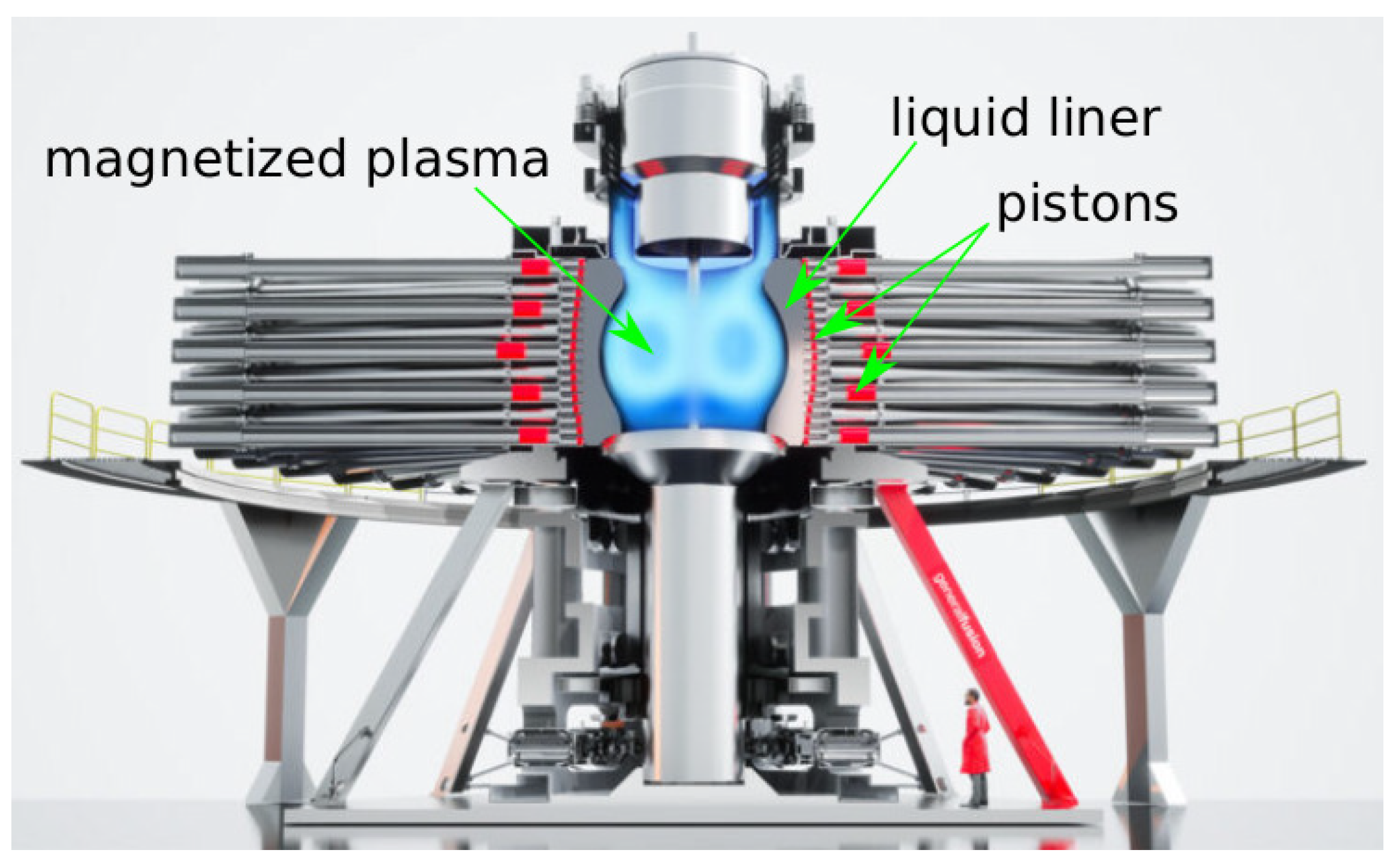
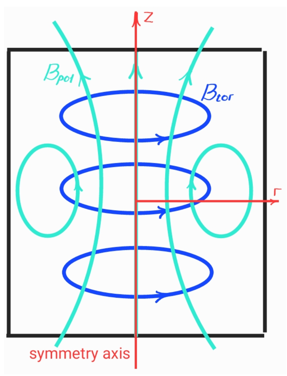
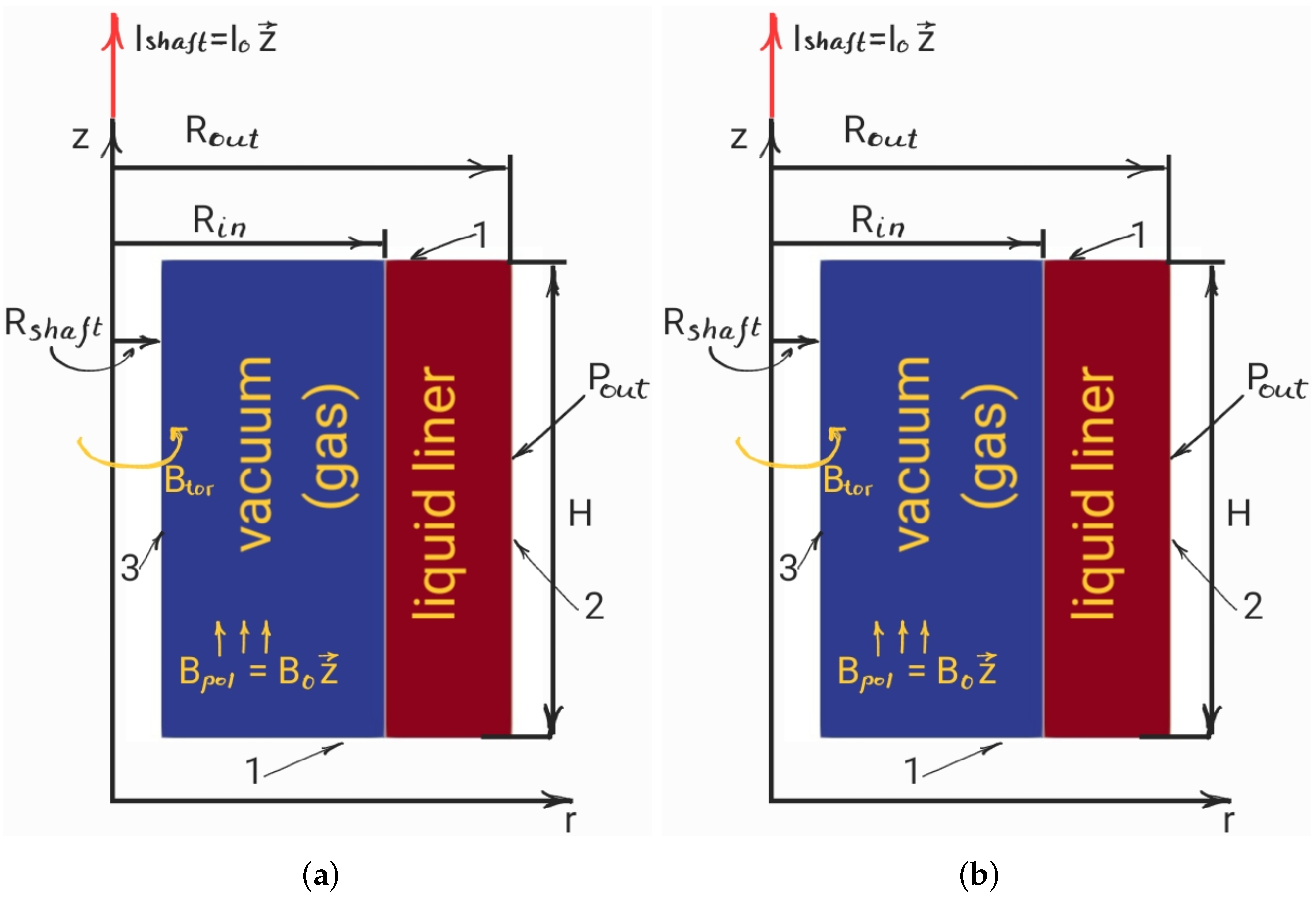
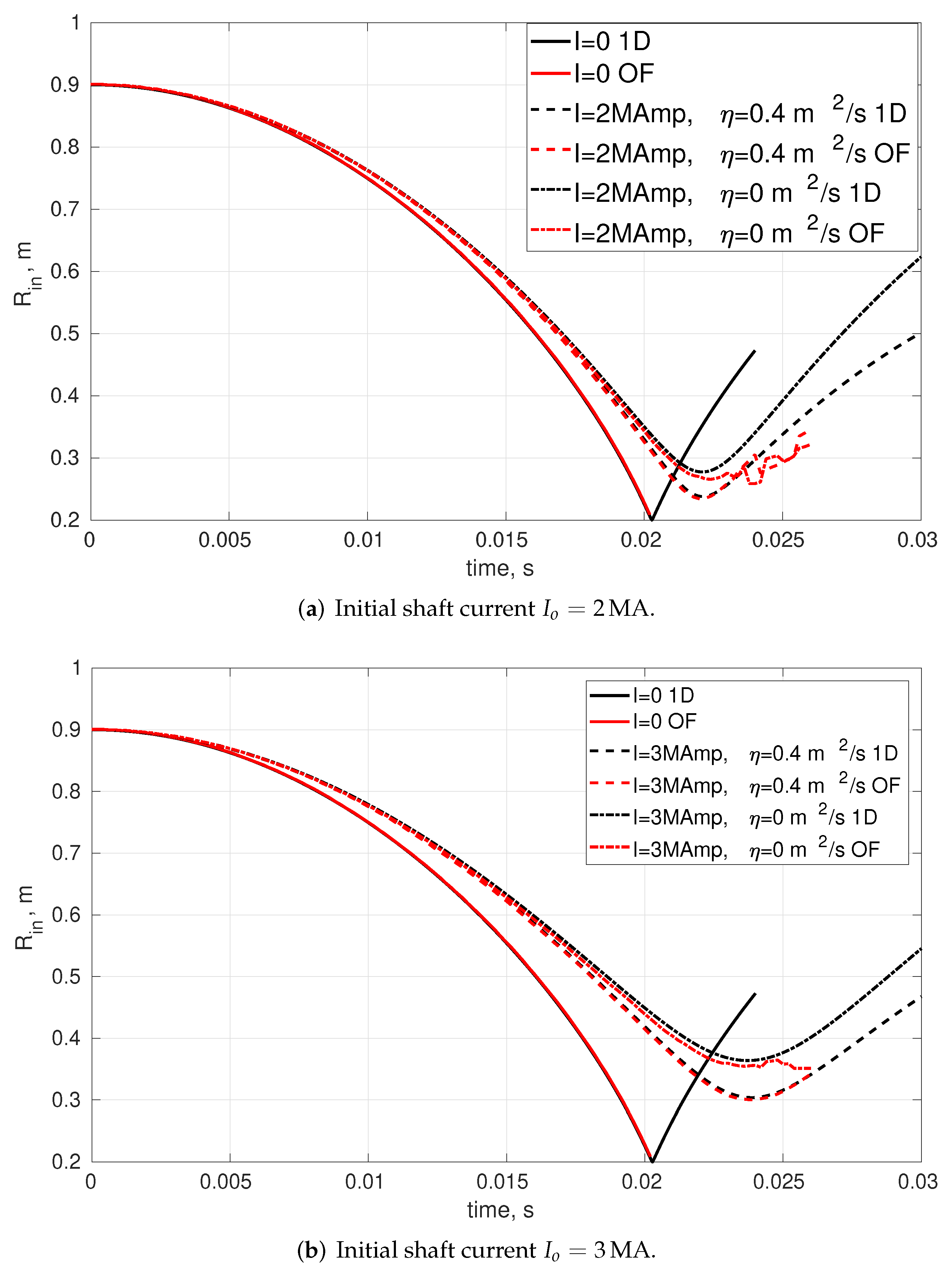
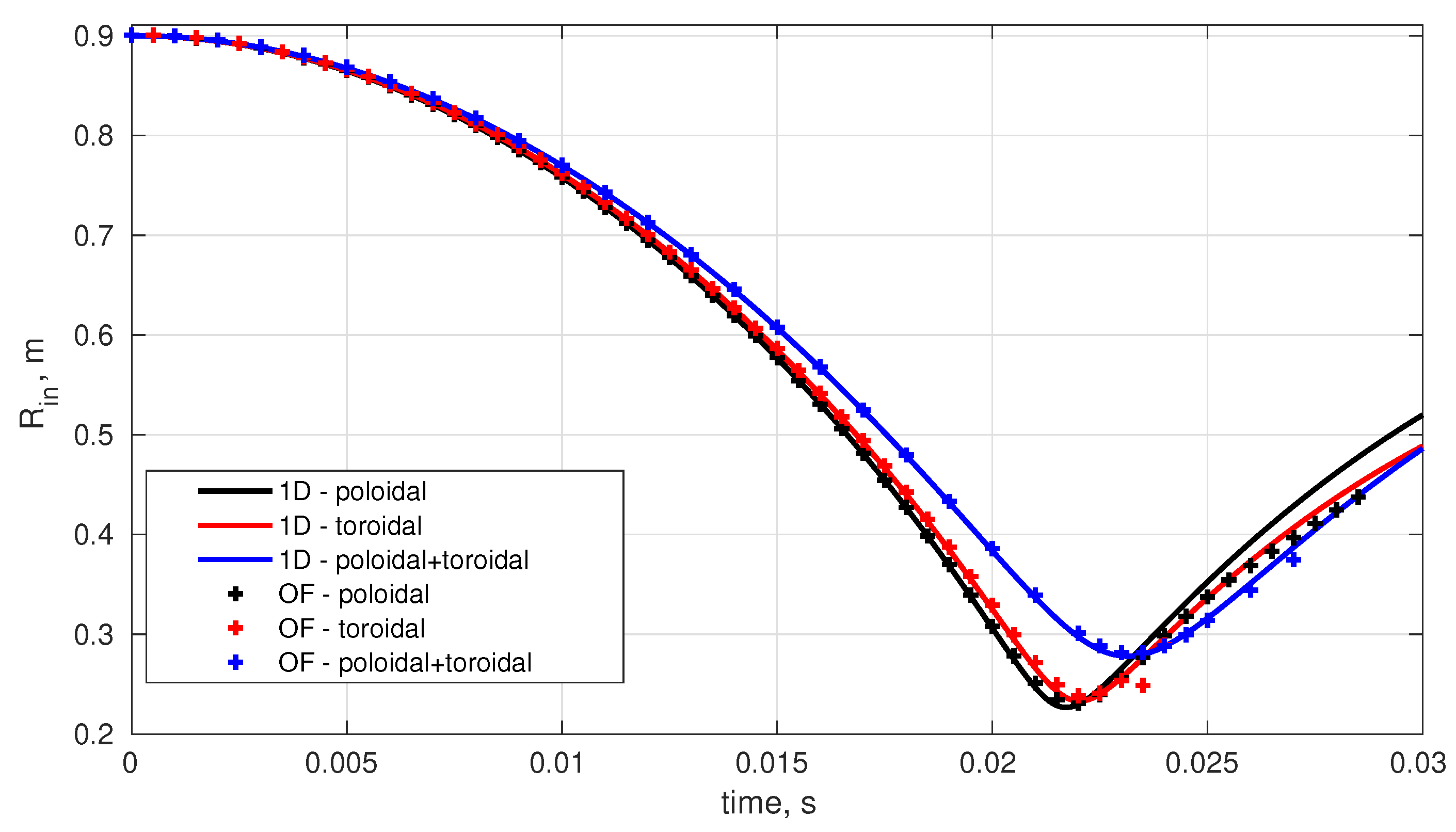
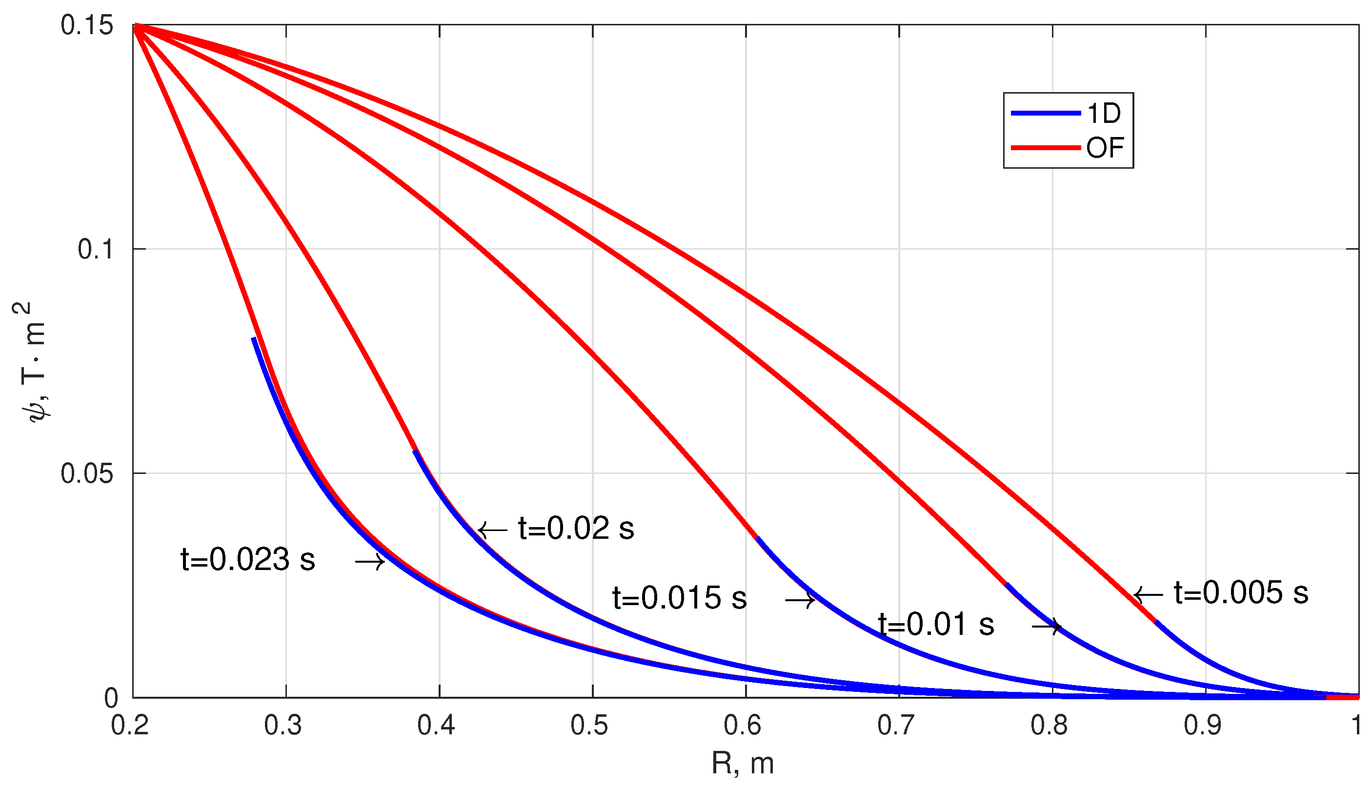
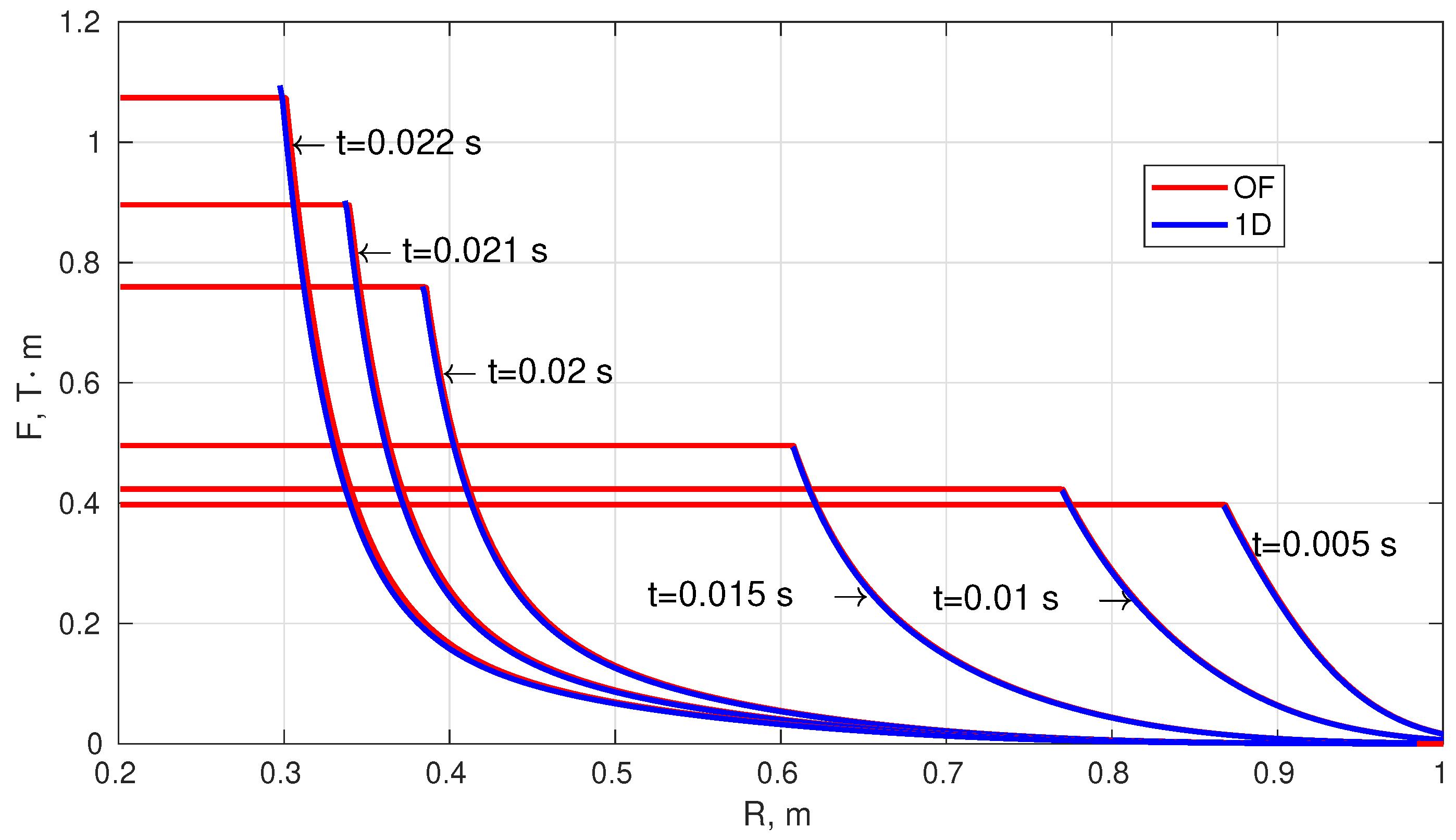
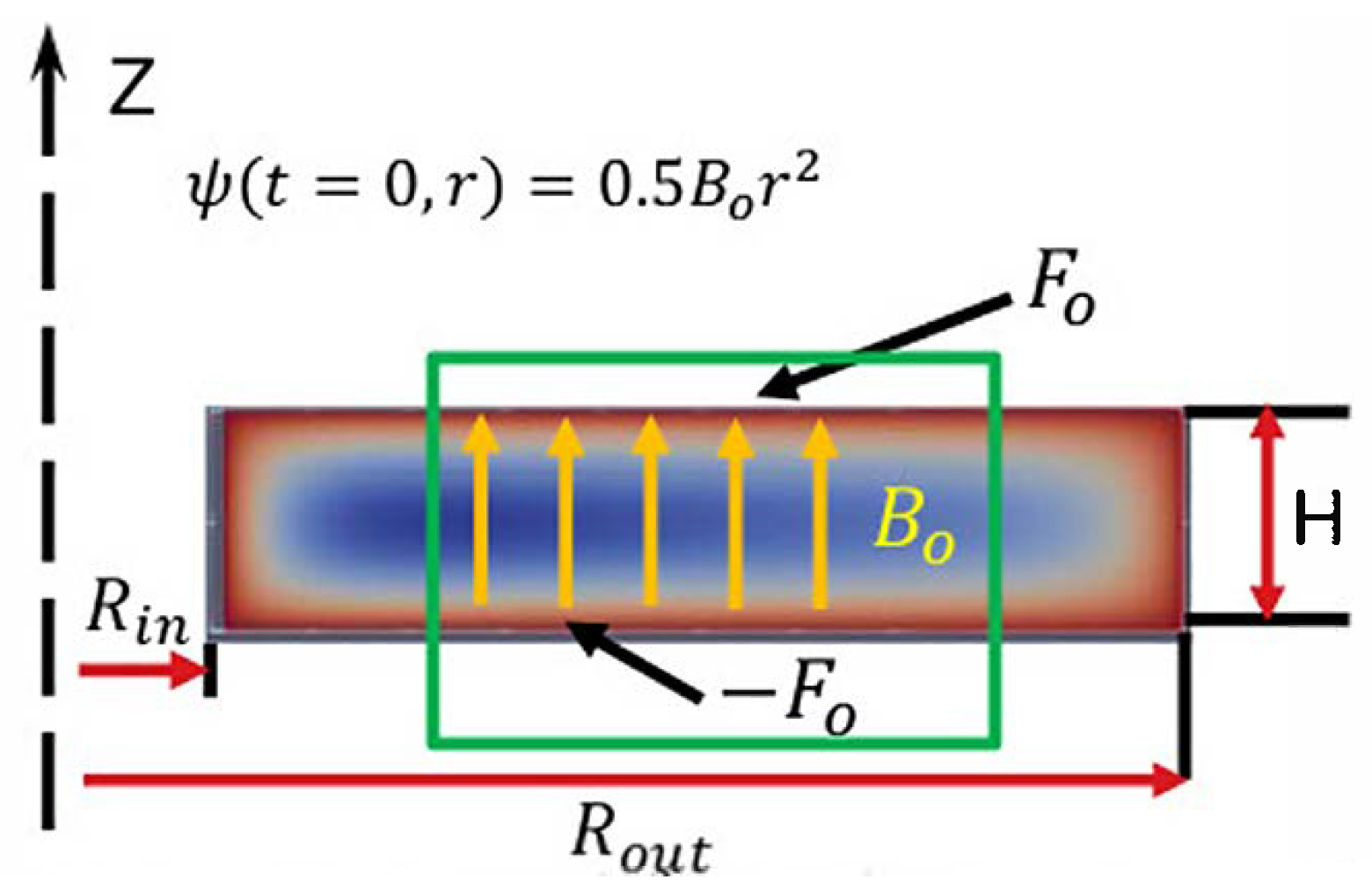
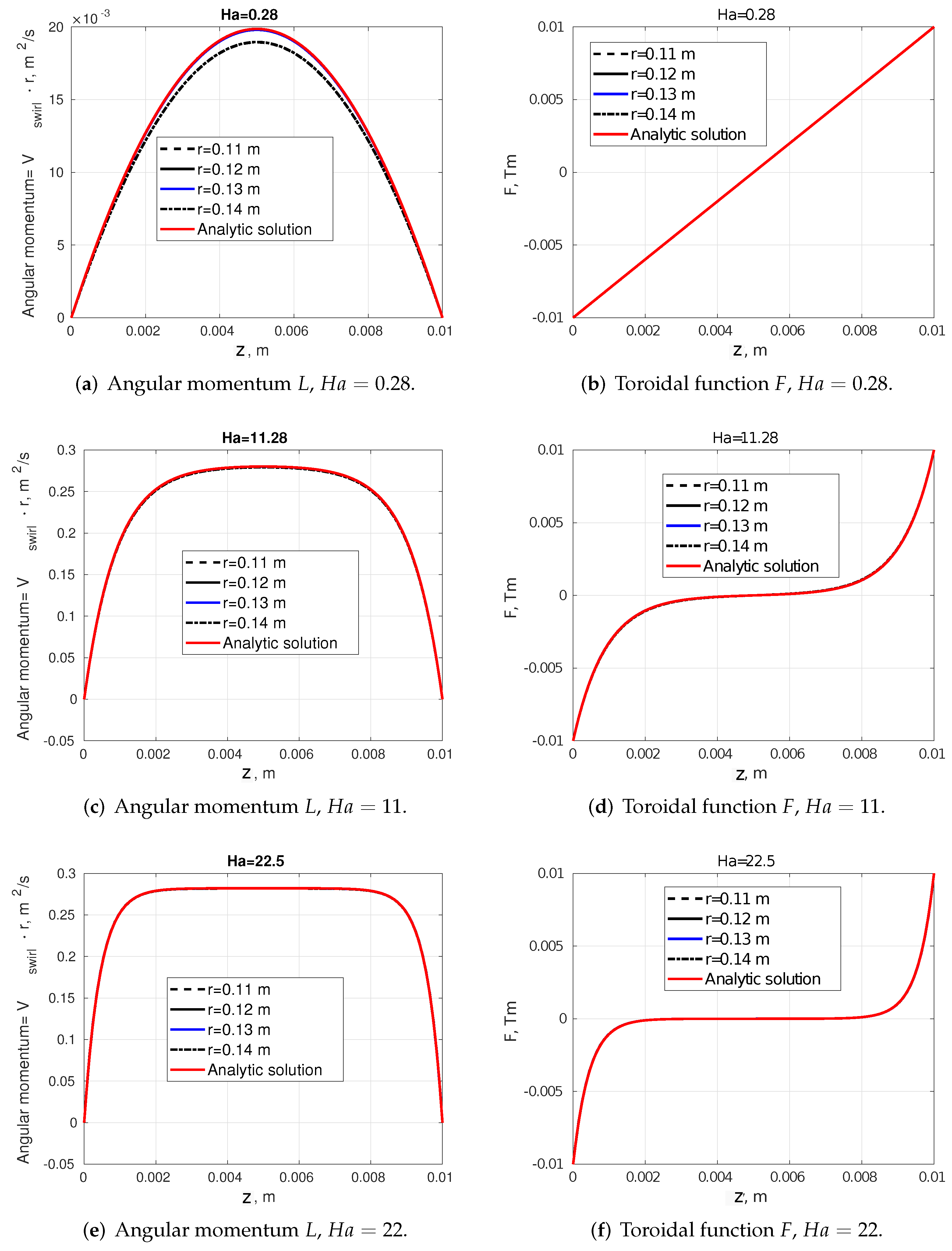
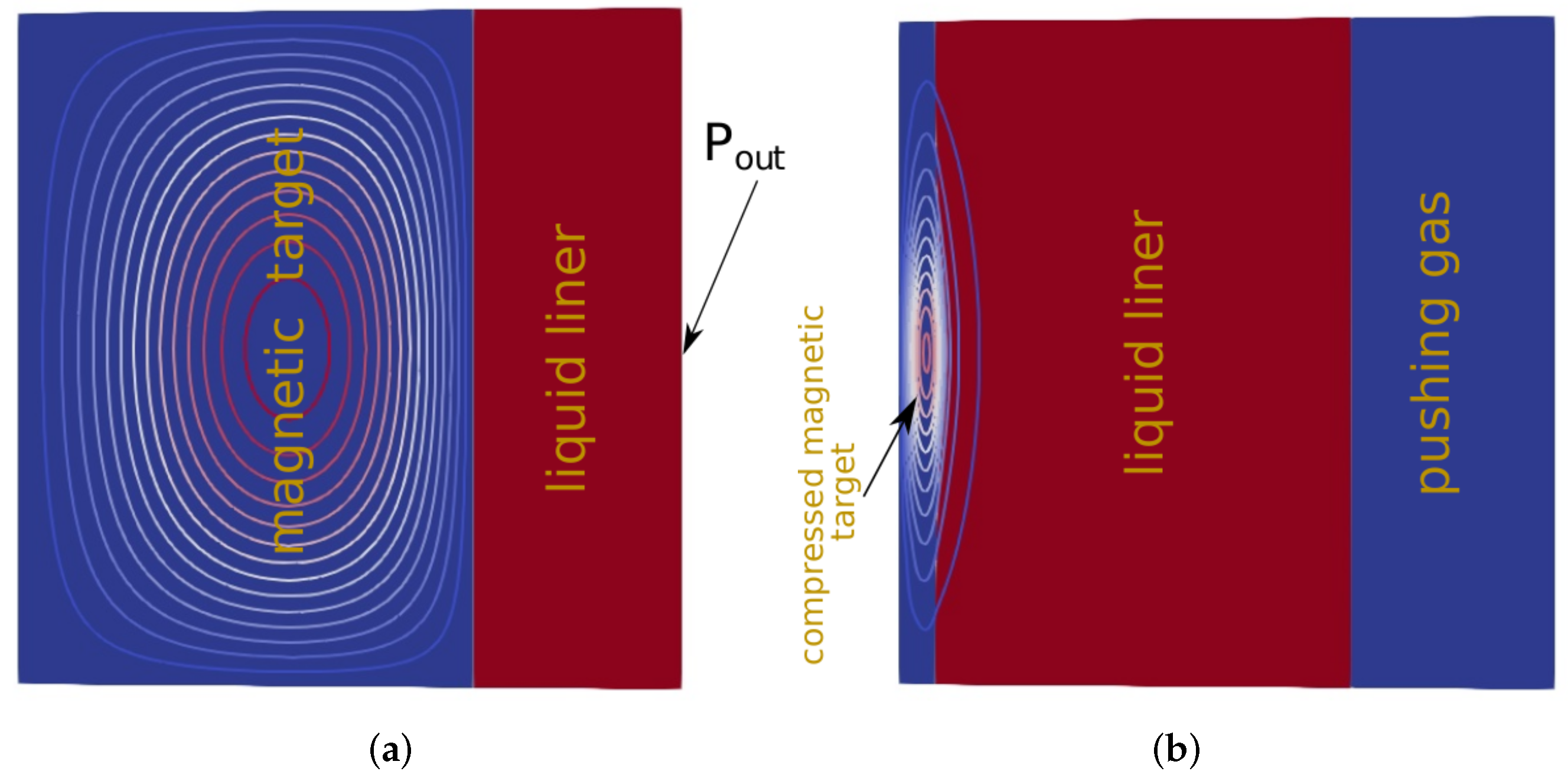
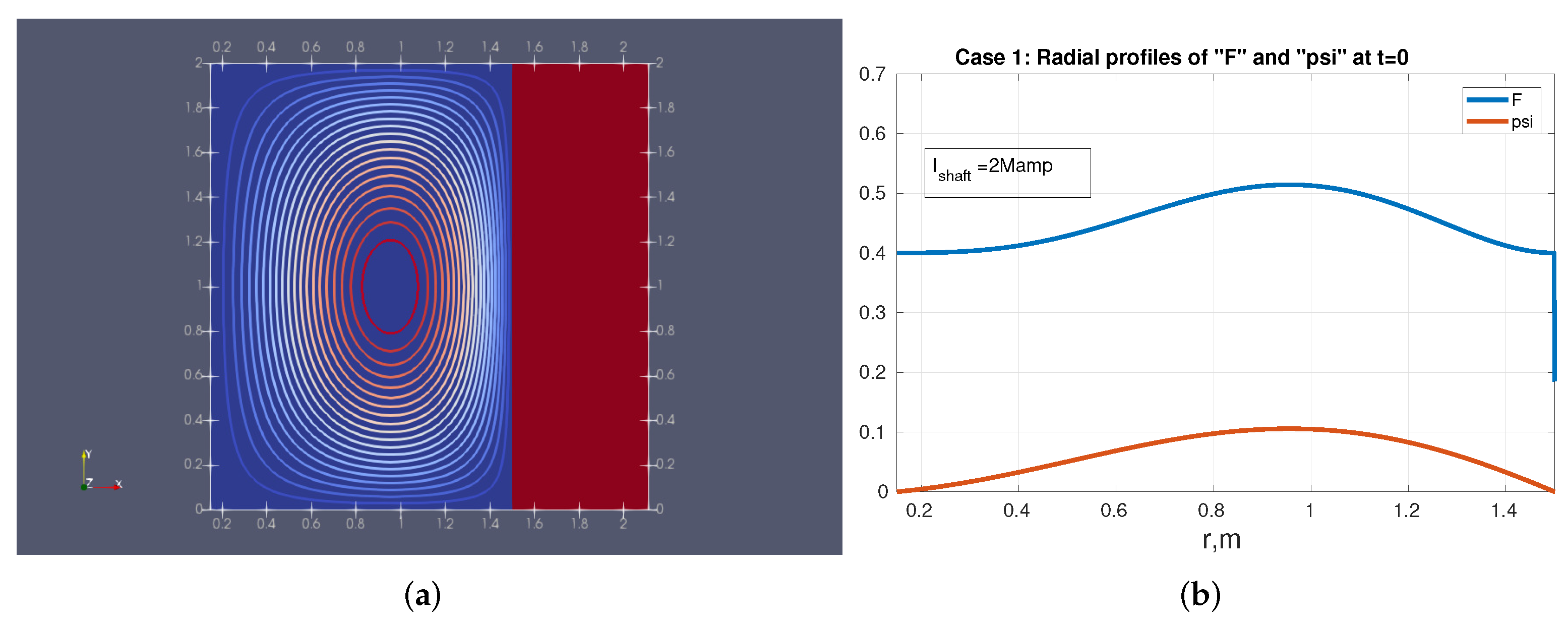
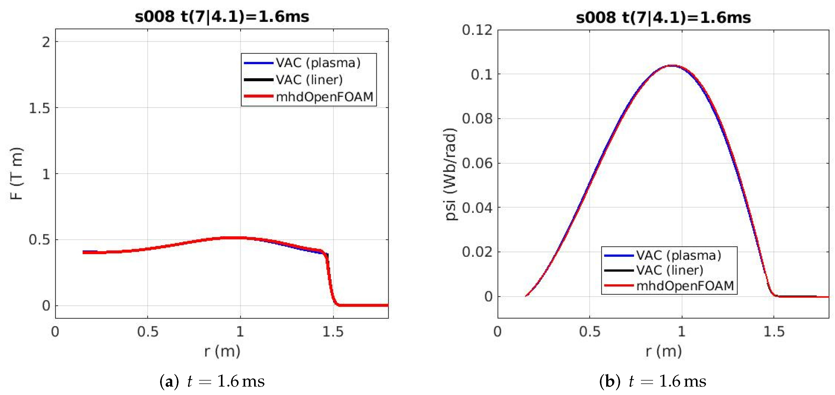
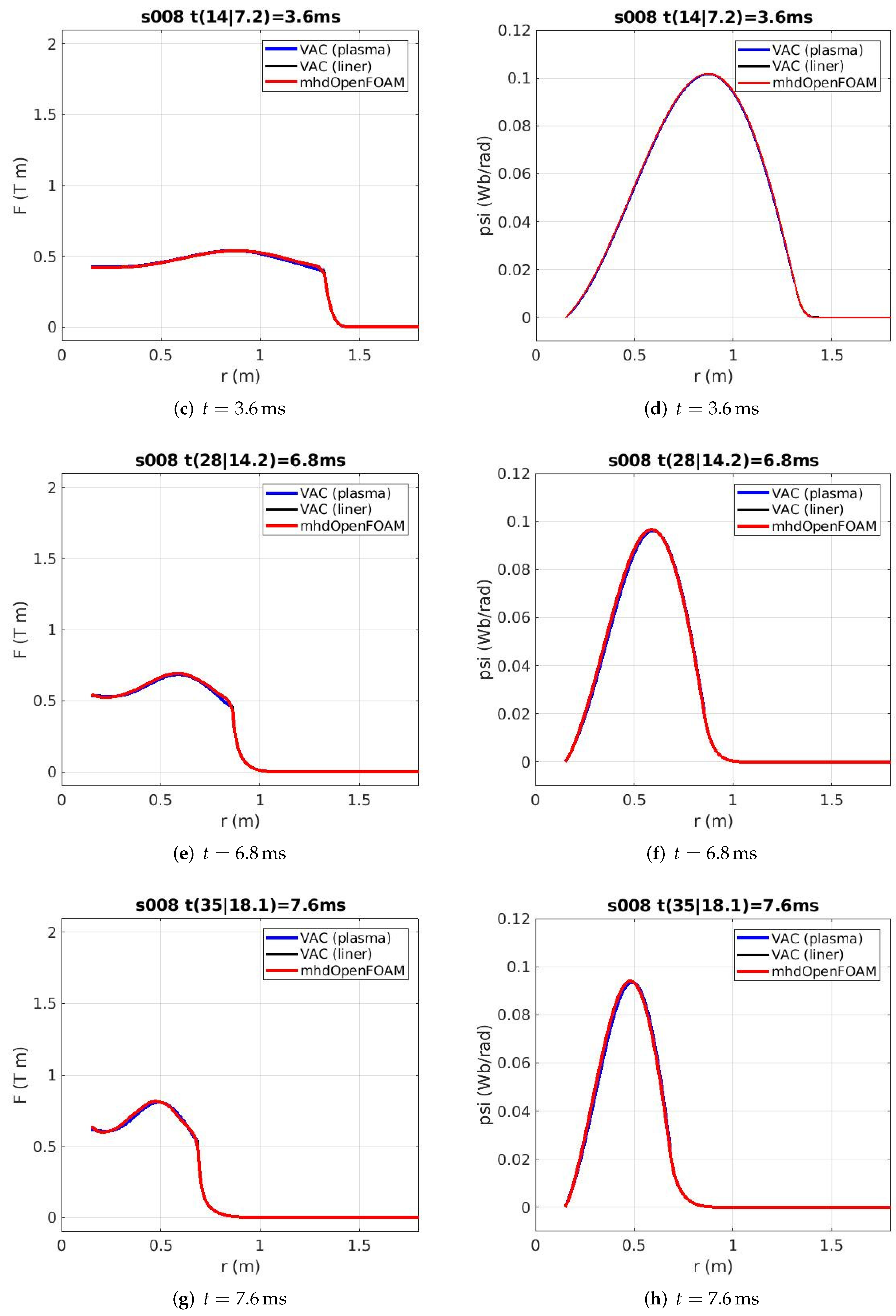
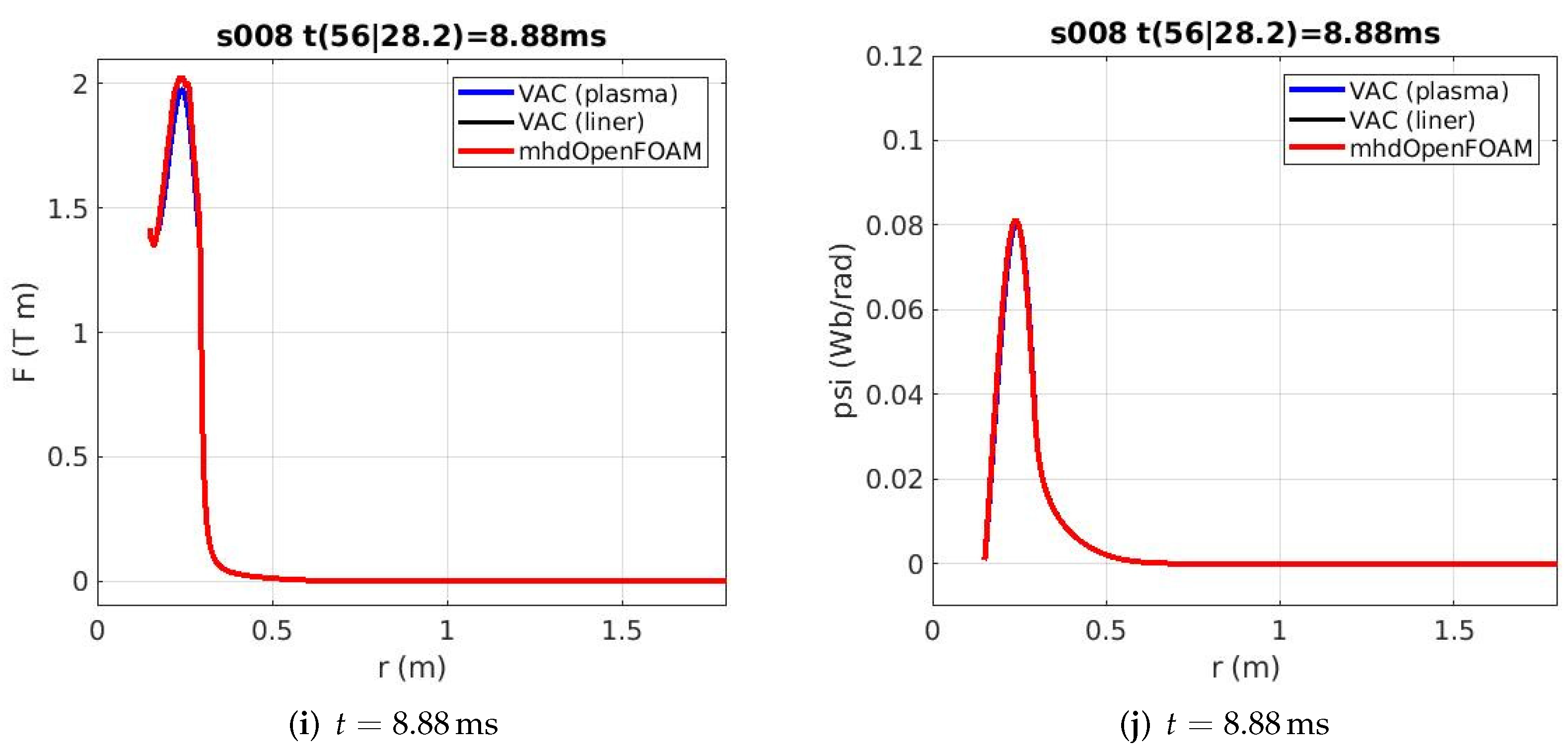
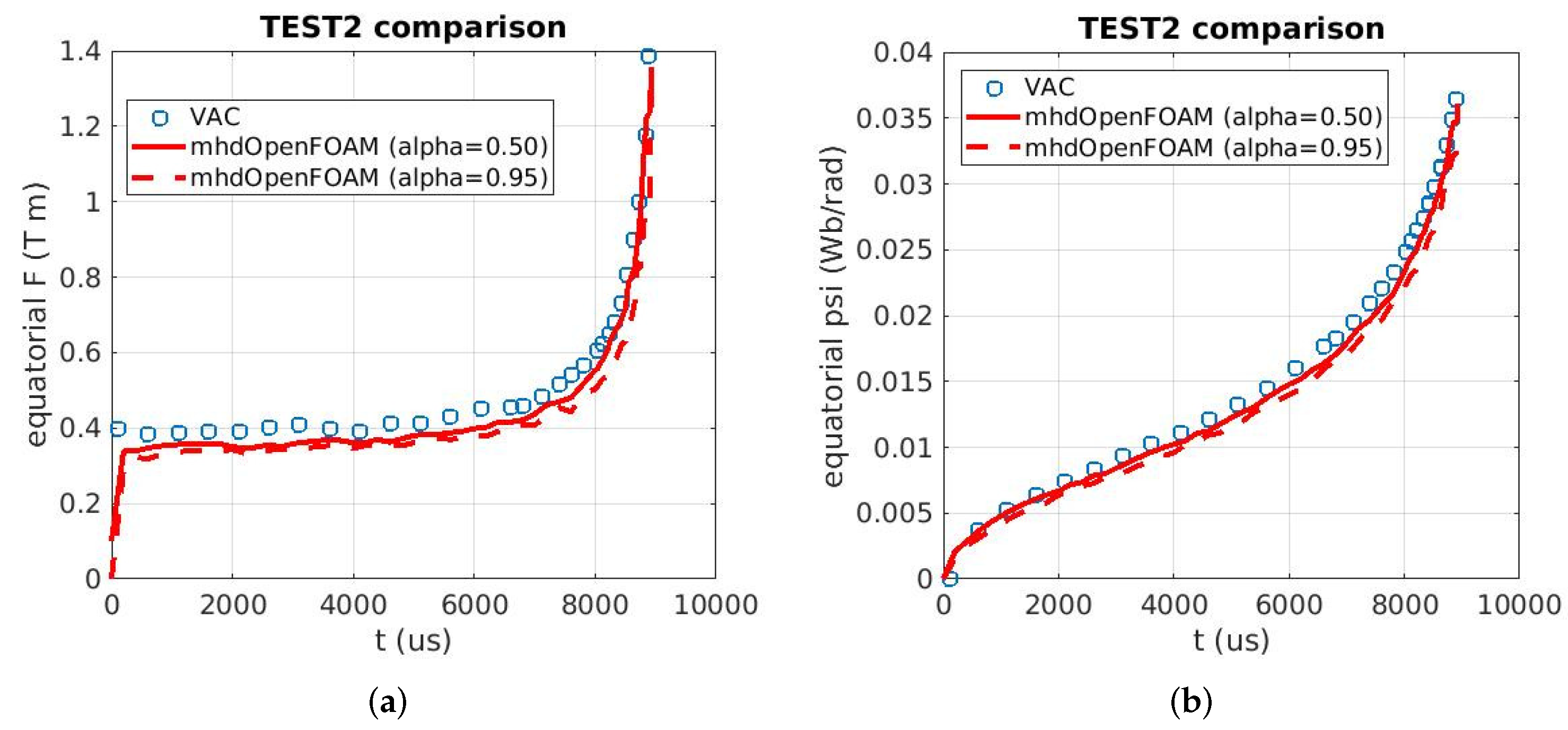
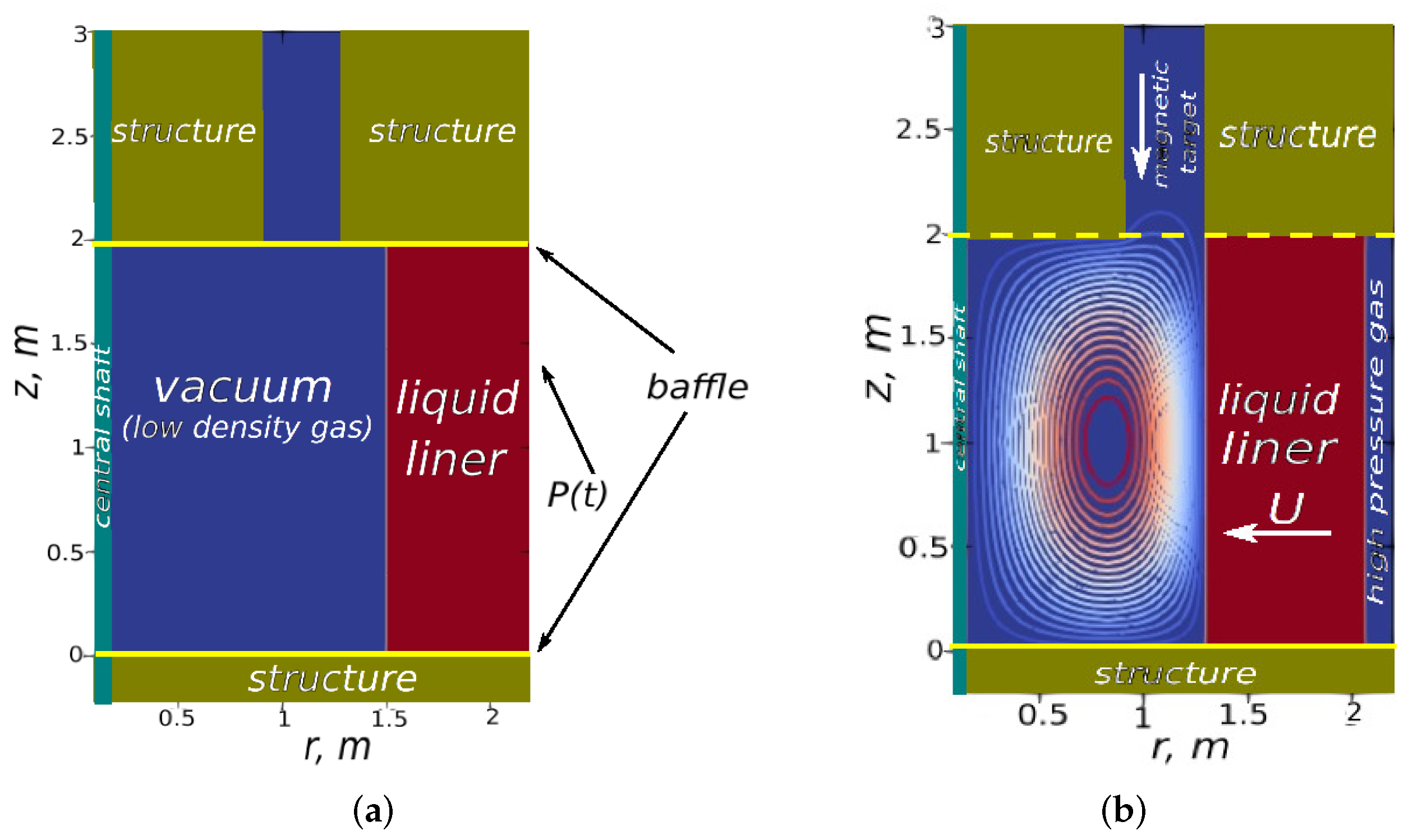
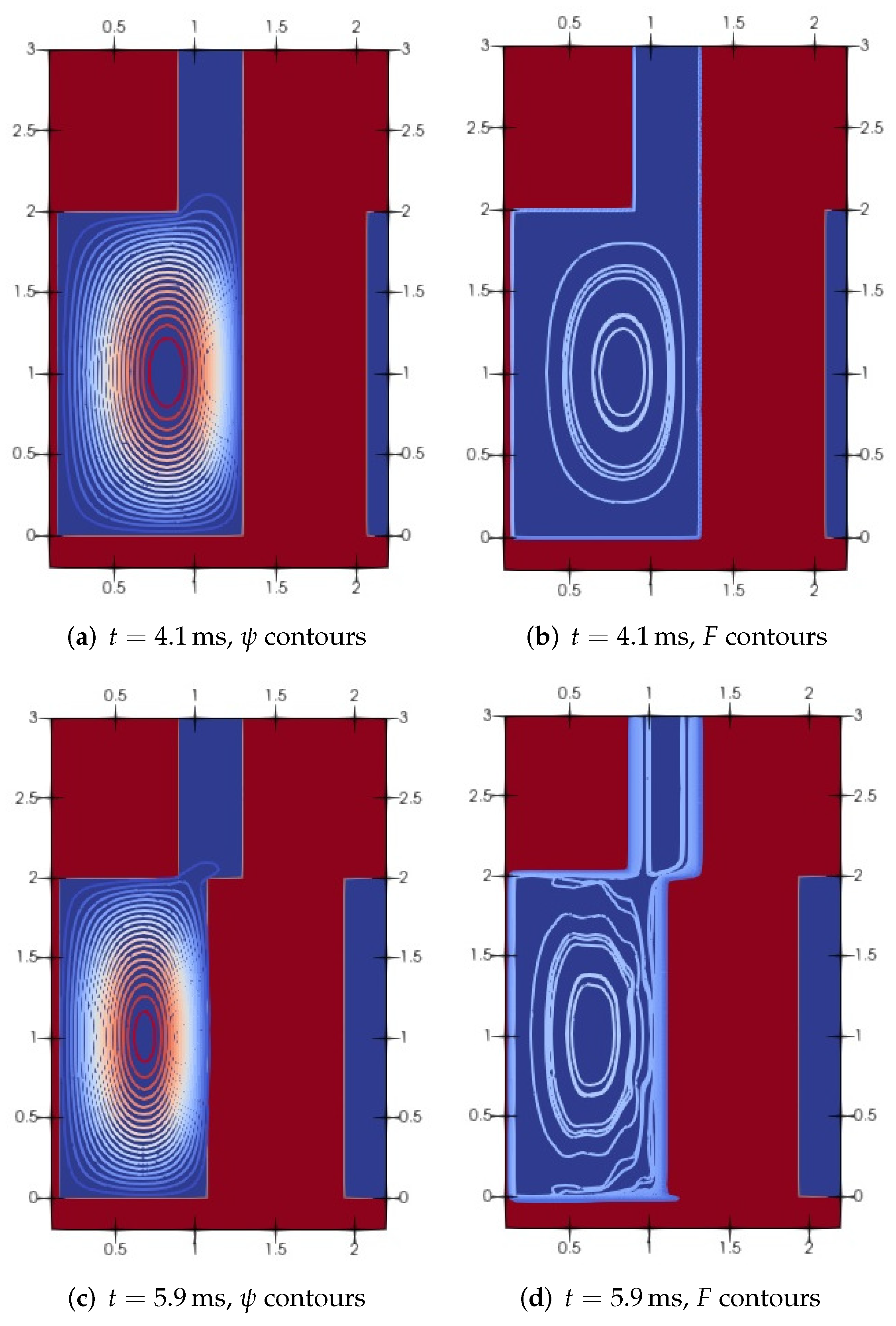
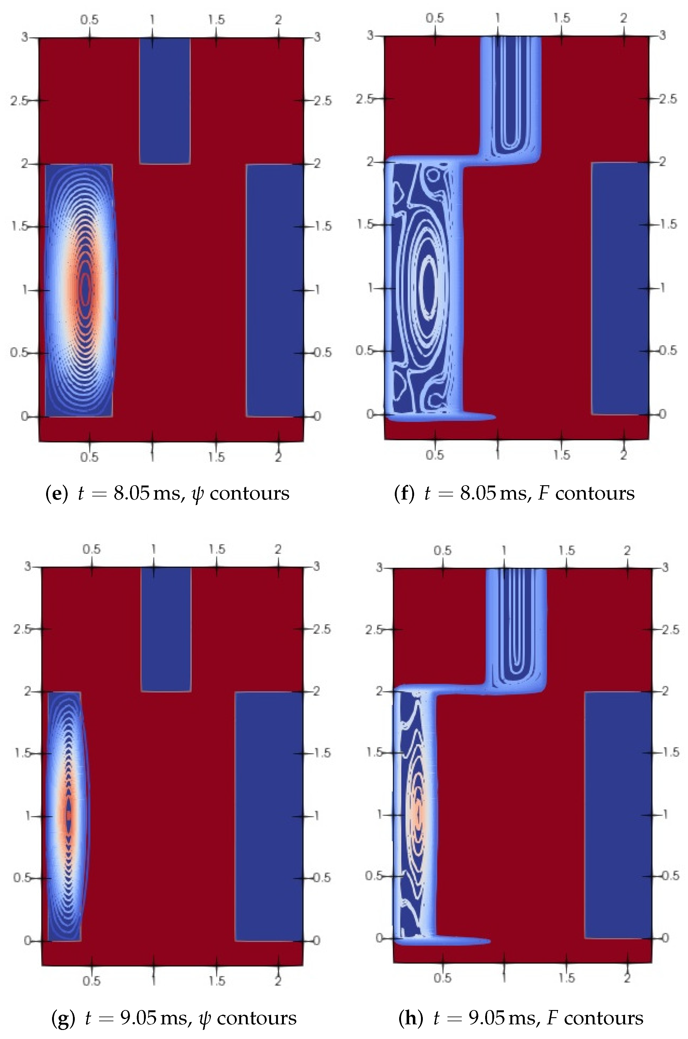
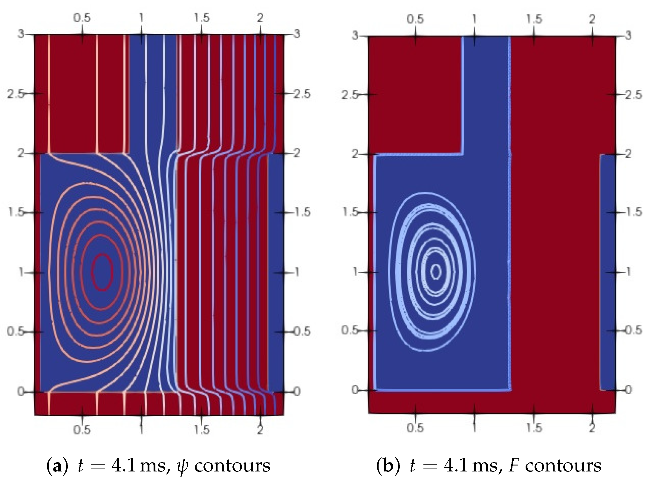
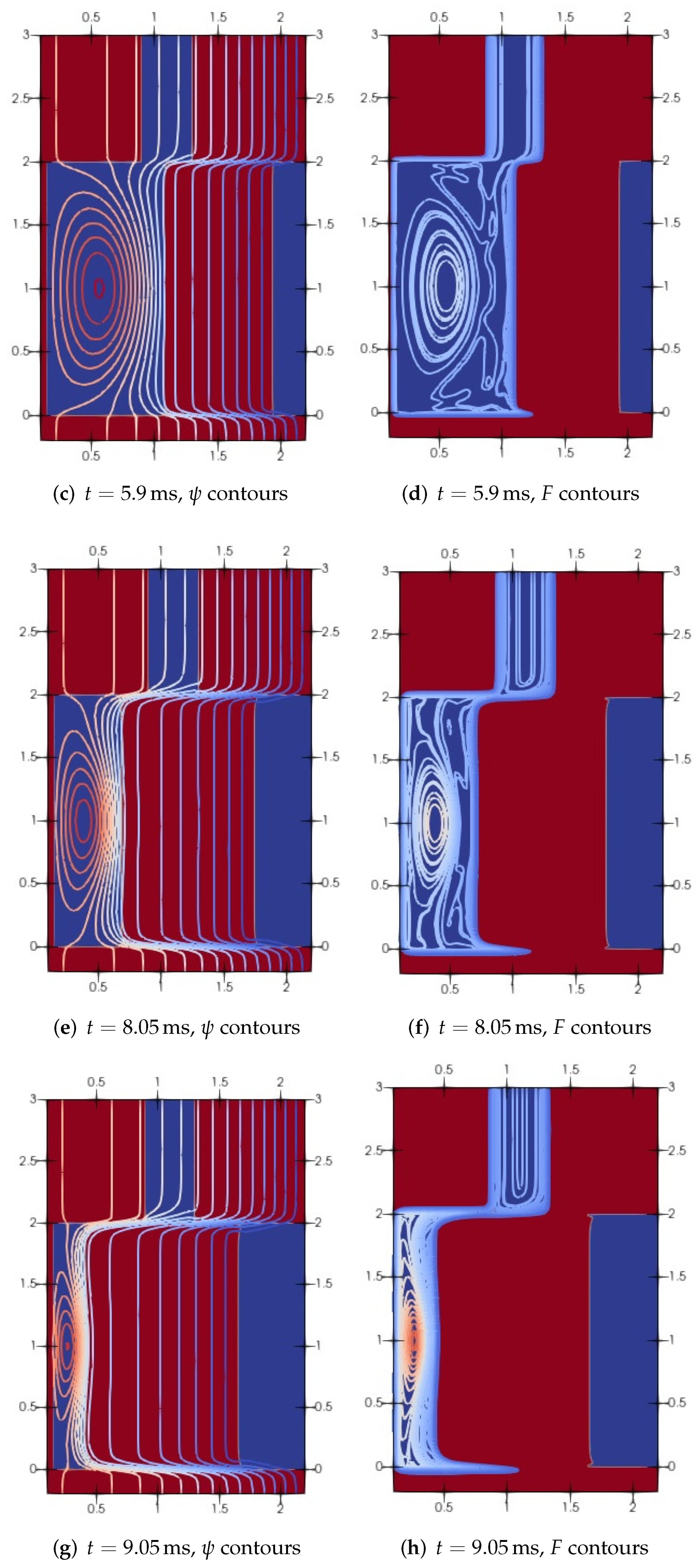
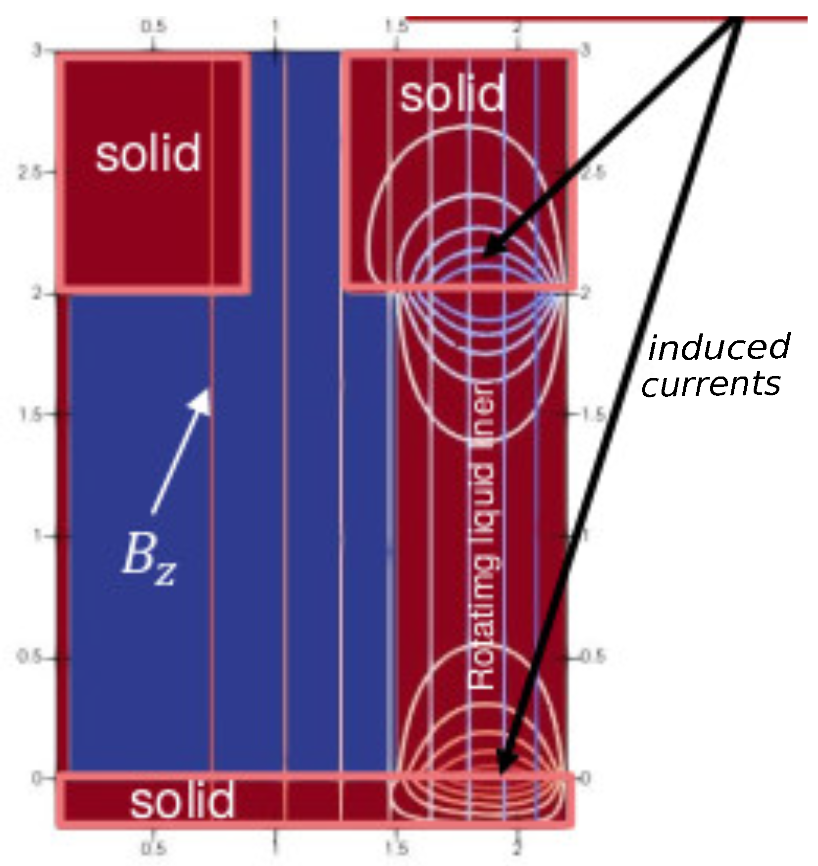
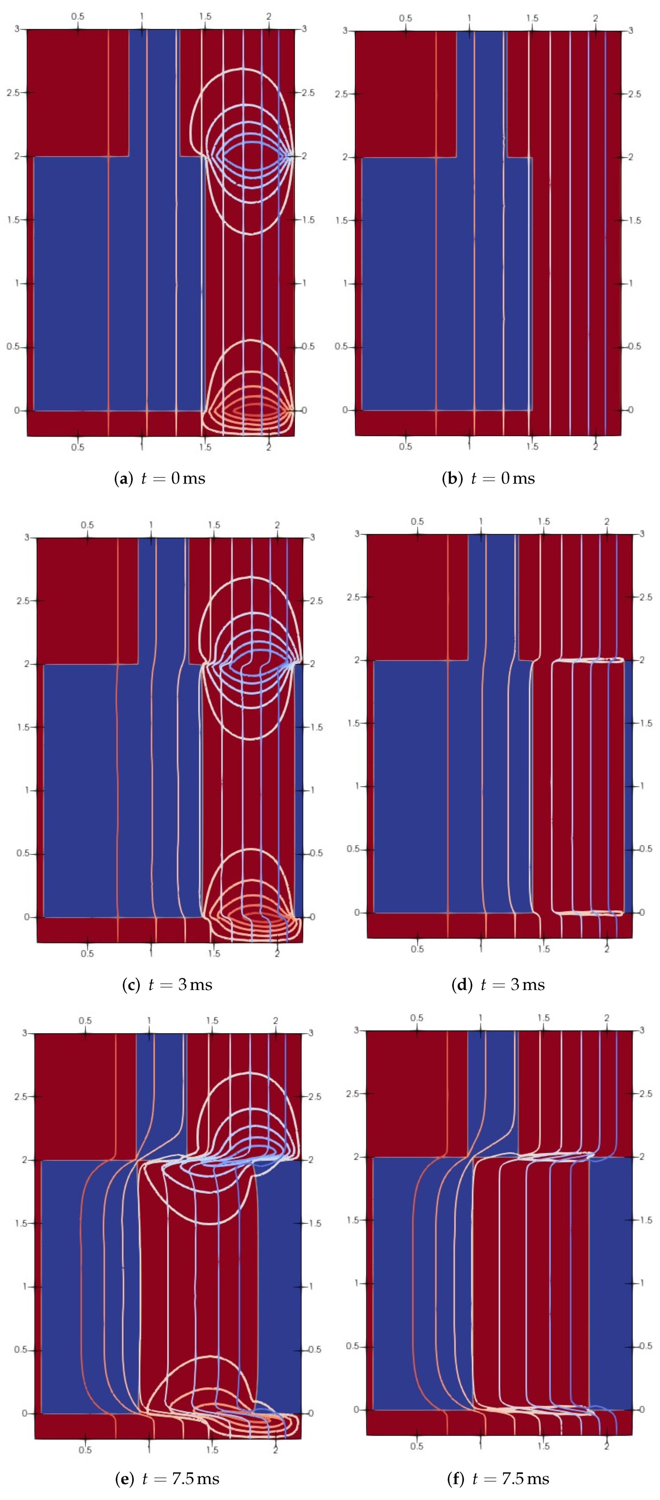
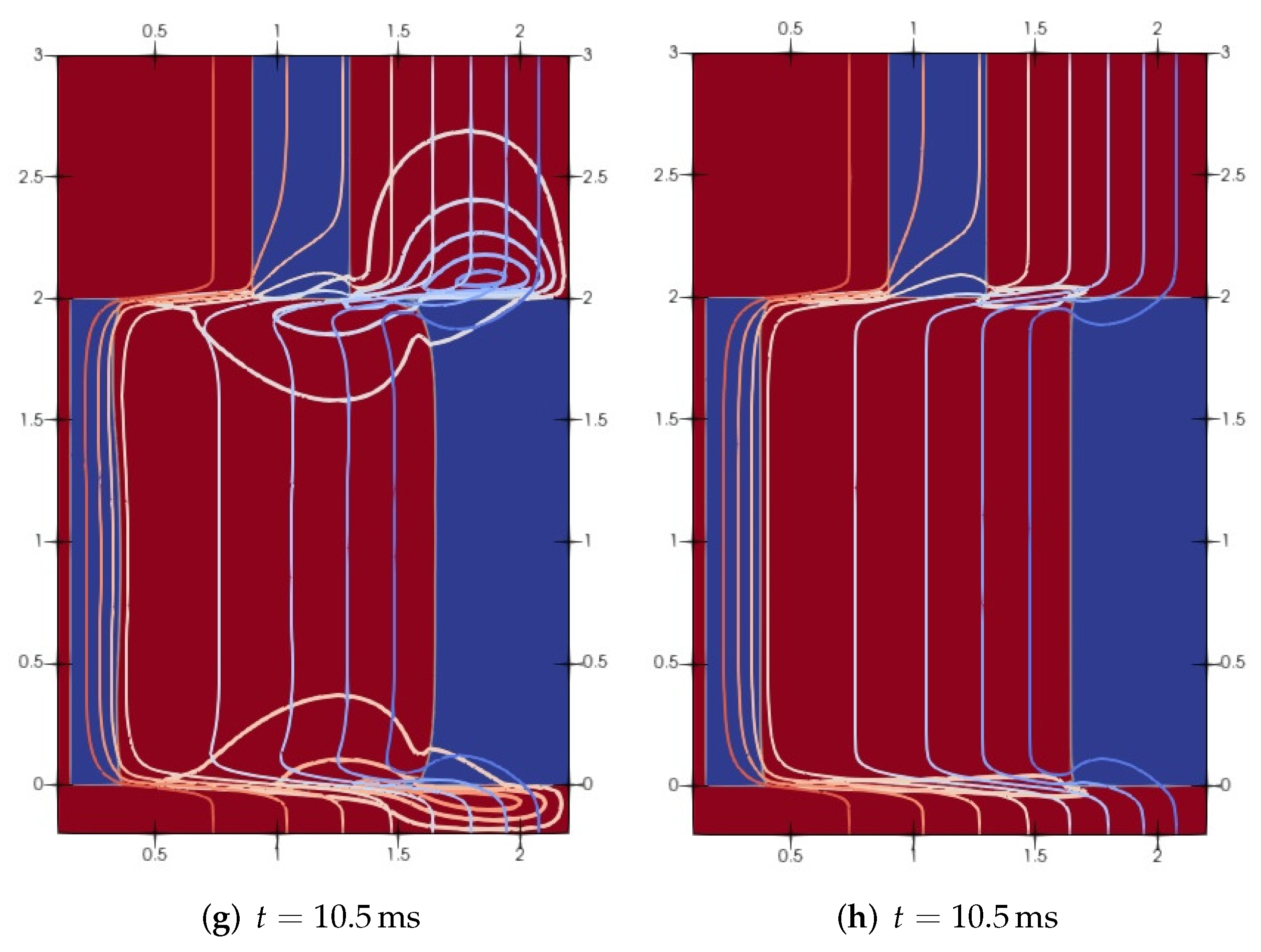
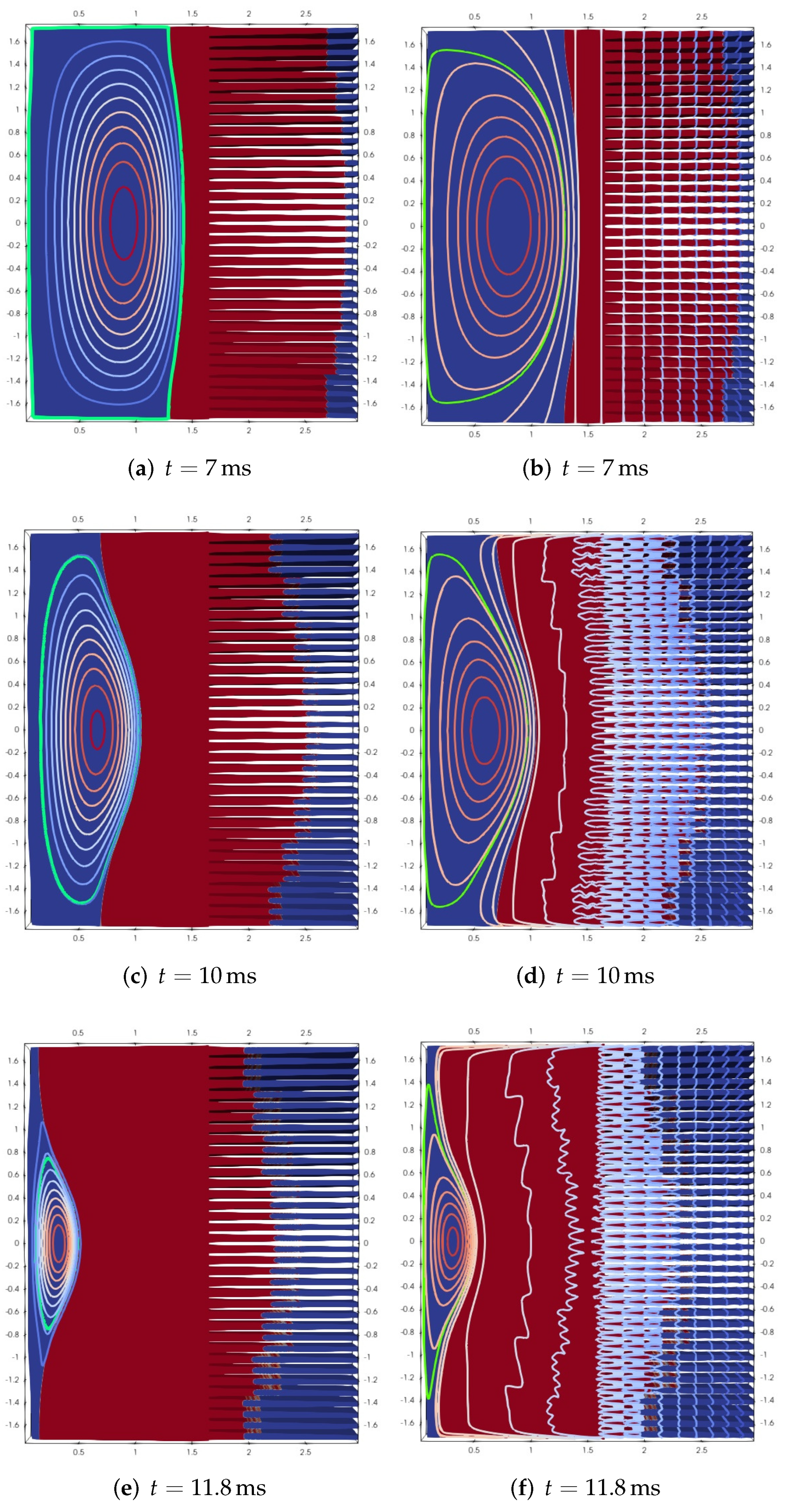
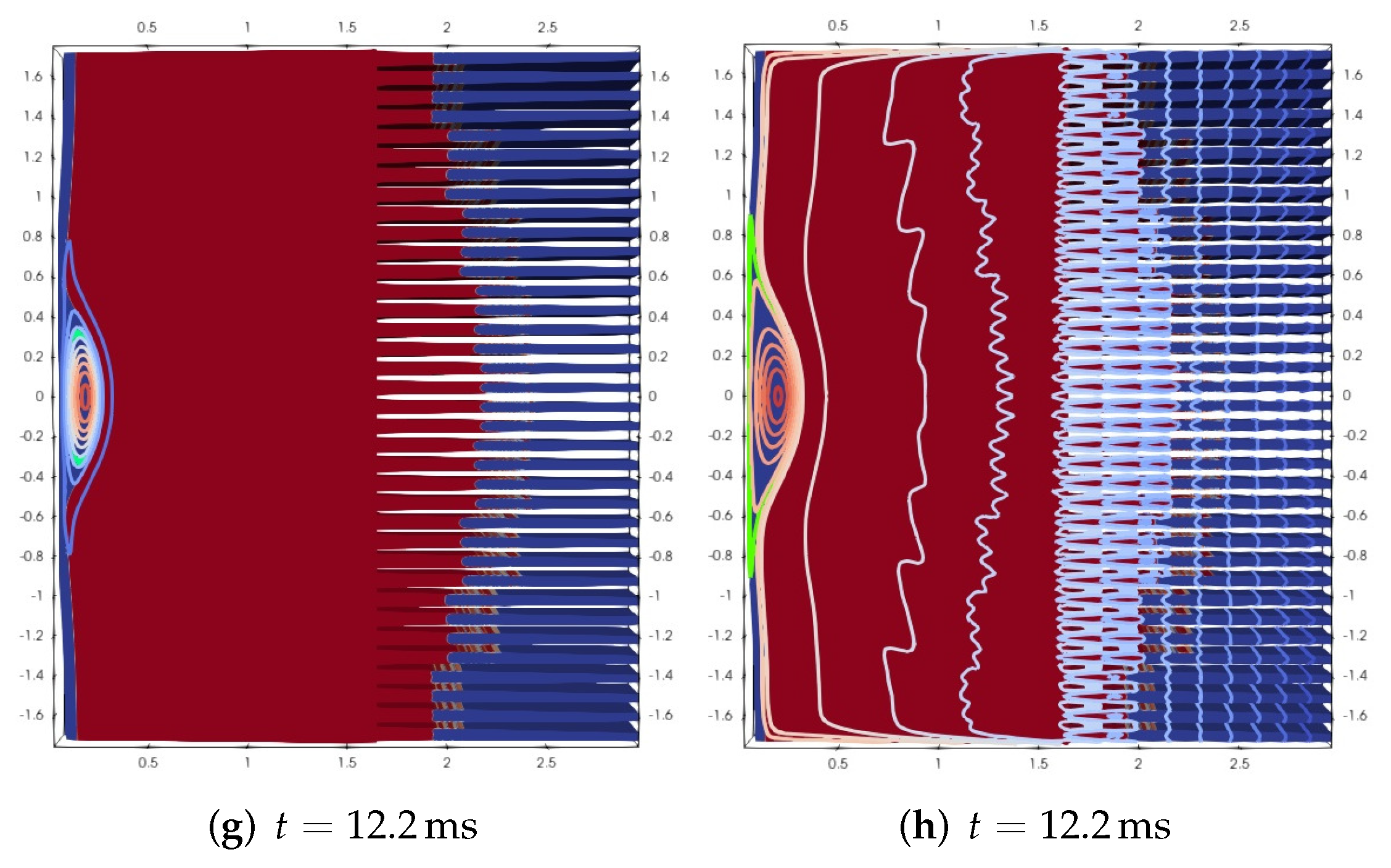
Table 1.
Test case parameters for comparison between “mhdCompressibleInterFoam” solver and “layered” VAC code.
Table 1.
Test case parameters for comparison between “mhdCompressibleInterFoam” solver and “layered” VAC code.
| Geometry | ||
|---|---|---|
| Shaft radius | ||
| Inner liner radius | ||
| Outer liner radius | ||
| Height of the liner | H | |
| Liquid liner (lithium) | ||
| Density | ||
| Viscosity | ||
| Magnetic diffusivity | ||
| EoS | constant density | |
| Pushing pressure | ||
| Magnetic target | ||
| Initial pressure (uniform) | ||
| Initial density (uniform) | ||
| Viscosity | ||
| Magnetic diffusivity (constant) | ||
| Initial magnetic configuration | ||
| Shaft current | ||
| Maximum poloidal flux (per radian) | ||
| Parameters in Equations (27) and (28) | ||
| Wave number | k | |
| Eigenvalue | ||
| Amplitude constant | c | |
| Shaft current constant | ||
| Simulation type | ||
| Laminar, iso-thermal, high target viscosity, constant magnetic diffusivity | ||
Table 2.
Case parameters for the setup including solid regions (see Figure 14).
Table 2.
Case parameters for the setup including solid regions (see Figure 14).
| Geometry | ||
|---|---|---|
| Shaft radius | ||
| Inner liner radius | ||
| Outer liner radius | ||
| Height of the liner | H | |
| Solid regions | , , , | |
| Injection opening | , | |
| Liquid liner (lithium) | ||
| Density | ||
| Viscosity | ||
| Magnetic diffusivity | ||
| EoS | constant density | |
| Pushing pressure | ||
| Magnetic target | ||
| Initial pressure (uniform) | ||
| Initial density (uniform) | ||
| Viscosity | ||
| Magnetic diffusivity (constant) | ||
| Initial magnetic configuration—Grad-Shafranov equilibrium (injected in ) | ||
| Shaft current | ||
| Maximum poloidal flux (per radian) | ||
| Shaft current constant | ||
| Simulation type | ||
| Laminar, iso-thermal, high target viscosity, constant magnetic diffusivity | ||
Publisher’s Note: MDPI stays neutral with regard to jurisdictional claims in published maps and institutional affiliations. |
© 2022 by the authors. Licensee MDPI, Basel, Switzerland. This article is an open access article distributed under the terms and conditions of the Creative Commons Attribution (CC BY) license (https://creativecommons.org/licenses/by/4.0/).
Share and Cite
MDPI and ACS Style
Suponitsky, V.; Khalzov, I.V.; Avital, E.J. Magnetohydrodynamics Solver for a Two-Phase Free Surface Flow Developed in OpenFOAM. Fluids 2022, 7, 210. https://0-doi-org.brum.beds.ac.uk/10.3390/fluids7070210
AMA Style
Suponitsky V, Khalzov IV, Avital EJ. Magnetohydrodynamics Solver for a Two-Phase Free Surface Flow Developed in OpenFOAM. Fluids. 2022; 7(7):210. https://0-doi-org.brum.beds.ac.uk/10.3390/fluids7070210
Chicago/Turabian StyleSuponitsky, Victoria, Ivan V. Khalzov, and Eldad J. Avital. 2022. "Magnetohydrodynamics Solver for a Two-Phase Free Surface Flow Developed in OpenFOAM" Fluids 7, no. 7: 210. https://0-doi-org.brum.beds.ac.uk/10.3390/fluids7070210