Drag Reduction by Wingtip-Mounted Propellers in Distributed Propulsion Configurations

Abstract

Tip-mounted propellers can increase wing aerodynamic efficiency, and the concept is gaining appeal in the context of hybrid electrical propulsion for greener aviation, as smaller and lighter electrical motors can help with mitigating structural drawbacks of a tip engine installation. A numerical study of tip propeller effects on wing aerodynamics is herein illustrated, considering different power configurations of a Regional Aircraft wing. A drag breakdown analysis using far-field methods is presented for one of the most promising configurations, and a comparison between drag reductions obtained with a tip propeller or a standard winglet installation is also provided. Numerical flow simulations using Finite Volume Methods with actuator disk models are compared with results of a Vortex-Lattice Method, and far-field aerodynamic force calculation is performed for different mesh sizes. A wing drag reduction up to 6% (10%) is predicted under typical cruise (climb) flight conditions when wingtip-mounted propellers take over half of the total thrust usually provided by turbo-prop engines installed at inboard wing position. Drag breakdown analysis confirmed that the observed benefits mainly come from a reduction in the reversible drag component, increasing the effective wing span efficiency.

1. Introduction

Regional transportation has historically been one of the aviation markets that best exploits the higher fuel efficiency offered by propeller-driven aircrafts compared to lower by-pass ratio turbojets, reducing pollutant emissions and confirming a key role for propeller propulsion technology in the context of greener aviation. Moreover, recent progresses in electric motors and battery technology, together with environmental requirements targeting climate neutrality, is pushing research toward more electric hybrid power-plant architectures [1] that provide higher flexibility to preliminary configuration designers. They indeed offer the possibility to distribute the propulsion system over the aircraft lifting surfaces using different, lower sized, electric motors, without the down-scaling efficiency issues typical of thermal engines [2]. This is useful, as wing–propeller interaction effects can be exploited in such a way to improve aircraft aerodynamic performance once knowledge of relevant power-plant/airframe integration aspects has been carefully addressed. Tip propeller installations, for example, allow for increasing the effective wing span efficiency when rotating in the direction counteracting wing tip vortices [3], with propeller slipstream rotational flow acting as a swirl recovery mean at wing tips, shifting the trailing vortex core outboard and increasing lift-over-drag ratio [4]. Indeed, this phenomenological interpretation is motivated considering the two main characteristics of a propeller slipstream flow affecting the lifting surface: dynamic pressure increase (blowing effect) and swirl velocity components (upwash/downwash effect). In conventional inboard propeller installations, swirl rotation produces nearly opposite effects on the two sides of the wing portion affected by propeller wake, and variations of local effective angles of attack of wing sections at both sides almost compensate. As a result, drag reduction benefits are lost when propellers are located inboard of the wing-tip [5]. Propellers installed at wing tips, instead, have a one-sided upwash effect on the outermost wing sections when rotating in the appropriate direction. On a lifting surface, local aerodynamic force vectors are tilted forward by propeller-induced upwash, in an opposite trend to wing drag due to lift (arising as a consequence of wing self-induced downwash), resulting in a reduction in wing reversible drag in power-on conditions [6]. So far, however, success of tip propeller installations has been strongly limited by structural issues mainly due to the high engine mass positioned outboard. Nowadays, hybrid electric architectures can help in mitigating the structural drawbacks of tip propeller configurations if smaller (and lighter) electric motors can be used at wing tips instead of heavier turbo generators.

A detailed characterization of wing–propeller interaction effects is therefore necessary in the perspective of designing novel regional aircraft configurations exploiting tip propeller drag-reduction benefits. Lots of research efforts have been spent in the past on the experimental characterization of wing–propeller interactions, with recent test campaigns taking advantage of Particle Image Velocimetry (PIV) measurement techniques applied to both inboard and outboard propeller installations [3,7]. Numerical studies using simplified analytical methodologies [8,9] or Computational Fluid Dynamic (CFD) techniques [10,11] have investigated different aspects of a single propeller installed inboard or at the wing tip. Results of CFD studies on drag reduction using multiple propellers are often available for Distributed Electric Propulsion (DEP) configurations without tip engines [12]. The focus of this paper is instead a multi-fidelity analysis of wing aerodynamic interaction with a two-propellers system, consisting of one propeller in the standard (reference) inboard position and the other one at wing tip, for different tip propeller diameters and operational conditions. The impact of the propellers’ slipstream on wing spanwise loading is analyzed and, for the reference configuration driven by one inboard propeller only (per half wing), drag reductions obtained using a classical tip winglet are compared to those obtained when part of the required thrust is delivered by an additional tip propeller. Finally, a drag breakdown analysis using thermodynamic far-field methods is performed for one of the most interesting power configurations analyzed in the document.

2. Methods

Wing–propeller aerodynamic interactions were analyzed using two numerical approaches: a higher fidelity Finite Volume Method (FVM) solving Reynolds-Averaged Navier–Stokes equations (RANS) and a lower-fidelity Vortex-Lattice Method (VLM) based on potential flow equations. This choice was motivated by the intention to set-up a simulation framework suitable for the preliminary aircraft design process, where quicker, lower-fidelity analyses of several configurations and/or power arrangements are appreciated but higher-fidelity simulations at selected design points are necessary to check the accuracy of fast methods and to allow for their fine tuning. A detailed post-processing using far-field methods for the aerodynamic force calculation and decomposition was then applied to some FVM flow solutions.

2.1. Finite Volume Method

An RANS formulation of flow-governing equations is used, with turbulence closure based on k-$\omega$ SST Menter’s model [13]. RANS equations are solved down to the wall around wing surfaces (no wall functions), and the effect of each propeller on wing aerodynamics is simulated using an Actuator Disk (AD) model with propellers assumed to operate in axial flow conditions at any of the analyzed incidence angles.

The use of an AD model was motivated by a compromise between accuracy of results and computational cost. Full blade-resolving techniques have been successfully employed in similar problems, even being limited to steady simulations using rotating mesh domains [14]. Nevertheless, the applicability of actuator disk models to reduce the computational effort of more expensive, fully resolved blade simulations (steady or unsteady) is investigated, for example in a very accurate accurate way in [15], and is common practise in CFD analyses where simulating the effects of propeller slipstream on the airframe is the main goal [12,16]. The actuator disk surface, in this case, coincides with an internal boundary in the computational grid and user’s specified radial distributions of blades axial forces’ (thrust) shaft power and radial forces over the disk surface are provided as an input.

No-slip adiabatic conditions were assumed at solid walls and characteristics-based far-field conditions were applied at the external boundaries of the computational domain, with exception of the symmetry plane where a reflection boundary condition was assumed. Free-stream conditions included a Turbulent Intensity Level (TIL) set at $1\%$ of mean flow velocity and a turbulent-to-laminar viscosity ratio equal to 10.

Fully turbulent steady solutions were computed using two different flow solvers: CIRA in-house-developed ZEN code [17] and Stanford University Unstructured (SU2) solver. In both cases, dry air with Sutherland viscosity law was assumed, considering no variation of specific heat capacities with static temperature.

CIRA ZEN code is a multi-block structured flow solver, based on a cell-centered formulation with central schemes and a Jameson-like artificial dissipation model [17,18]. Used in steady-state mode, the code adopts a solution procedure based on the pseudo-time marching concept, the relaxation operator consisting of an explicit multi-stage Runge–Kutta integration scheme. Convergence is accelerated by implicit residual averaging, local time stepping and multi-grid techniques.

SU2 is an open source, public domain, computational analysis and design software package launched by Stanford University including an unstructured RANS solver [19,20]. Flow simulations used version 6.2.0 “Falcon” of the code, featuring a variable-load actuator disk model, developed at the University of Naples “Federico II” by the Theoretical and Applied Aerodynamic Research Group [21]. It is very similar to the actuator disk model implemented in CIRA ZEN solver, and analogously provides the capability to specify radially variable input data. Flow simulations used an implicit pseudo-time marching and central Jameson–Schmidt–Turkel scheme [18].

2.2. Vortex-Lattice Method

The Nasa Vspaero [22] code is used to carry out the low-fidelity simulations presented in this work. Vspaero is a fast, linear, vortex lattice and panel solver that can be accurately and easily described for aero-propulsive analysis. This code is part of OpenVSP [22] parametric aircraft geometry tool and is available under the terms of the NASA Open Source Agreement. Discrete vortices are applied to each panel and then evaluated over the entire surface to obtain a pressure distribution and thus force. The flow over a section of panels behind a propeller can be analysed by implementing actuator disks into the solver [9]. In order to increase the accuracy of induced drag estimation, an external procedure based on a simple model of iteration between wing and propeller [23] is developed and integrated with the original code. This procedure is able to work starting from span-wise load distribution, which can be provided by Vspaero or a generic CFD software. In fact, the procedure is able to work on a planar wing only, but new features will be added in the near future.

2.3. Far-Field Force Method

The force analysis and breakdown has been performed by the far-field method proposed by Paparone and Tognaccini and detailed in [24]; fundamental formulae are here briefly recalled.

A turbulent, steady high-Reynolds-number compressible flow around an aircraft configuration is considered. Assuming a Cartesian reference system with the x-axis aligned with the asymptotic velocity, a straightforward application of the momentum balance equation provides the far-field drag expression:

$$D_{far}=-{\int }_{S_{far}}\left[\rho u(\mathit{V}·\mathit{n})+(p-p_{\infty })n_x\right]dS,$$

(1)

where $\rho$ is the fluid density, $\mathit{V}={[u,v,w]}^T$ is the local velocity, p is the pressure and subscript ∞ specifies free-stream conditions. $S_{far}$ is the outer boundary of the computational domain, $\mathit{n}={[n_x,n_y,n_z]}^T$ is the unit normal vector pointing outside the computational domain. Expanding in Taylor’s series the axial velocity defect expression with respect to the entropy variation $\mathsf{\Delta }s=s-s_{\infty }$ and taking into account second order terms at most, the entropy drag expression is obtained. In addition, taking into account the Gauss theorem, the entropy drag can be expressed by a volume integral:

$$D_{\mathsf{\Delta }s}=-V_{\infty }{\int }_{\mathsf{\Omega }}\nabla ·\left[\rho g(\mathsf{\Delta }s)\mathit{V}\right]d\mathsf{\Omega },$$

(2)

where $\mathsf{\Omega }$ is the flow domain and

$$g(\mathsf{\Delta }s)=f_{s1}\left(\frac{\mathsf{\Delta }s}{R}\right)+f_{s2}{\left(\frac{\mathsf{\Delta }s}{R}\right)}^2,$$

(3)

with R that is the gas constant and the coefficients $f_{s1}$ and $f_{s2}$ given by

$$f_{s1}=-\frac{1}{\gamma M_{\infty }^2},f_{s2}=-\frac{1+\left(\gamma -1\right)M_{\infty }^2}{2{\gamma }^2{M}_{\infty }^4},$$

(4)

($M_{\infty }$ is the free-stream Mach number and $\gamma$ is the ratio of specific heats).

The entropy drag takes into account the contributions associated with irreversible processes: viscous and wave drag. The domain $\mathsf{\Omega }$ can be decomposed as $\mathsf{\Omega }={\mathsf{\Omega }}_{visc}\bigcup {\mathsf{\Omega }}_{sw}\bigcup$${\mathsf{\Omega }}_{sp}$, where ${\mathsf{\Omega }}_{visc}$ is the boundary layer and the wake regions, ${\mathsf{\Omega }}_{sw}$ is the shock wave region, and ${\mathsf{\Omega }}_{sp}$ is the remaining part of the flow field. Therefore, the entropy drag can be decomposed in three components:

$$\begin{array}{c}\hfill D_{visc}=V_{\infty }{\int }_{{\mathsf{\Omega }}_{visc}}\nabla ·\left(\rho g\mathit{V}\right)d\mathsf{\Omega },\\ \hfill D_w=V_{\infty }{\int }_{{\mathsf{\Omega }}_{sw}}\nabla ·\left(\rho g\mathit{V}\right)d\mathsf{\Omega },\\ \hfill D_{sp}=V_{\infty }{\int }_{{\mathsf{\Omega }}_{sp}}\nabla ·\left(\rho g\mathit{V}\right)d\mathsf{\Omega }.\end{array}$$

(5)

$D_{visc}$ is the viscous drag, $D_w$ is the wave drag and $D_{sp}$ is the spurious drag component, linked to the numerical dissipation introduced by the numerical schemes that lead to a nonphysical drag contribution.

It is clear that the breakdown method relies on a proper selection of the three domains ${\mathsf{\Omega }}_{visc}$, ${\mathsf{\Omega }}_{sw}$ and ${\mathsf{\Omega }}_{sp}$. This is performed by the definition of boundary layer and shock-wave sensors discussed in [24,25]. Recently, Saetta and Tognaccini proposed a region identification based on a machine-learning algorithm independent of numerical input or thresholds [26]. Finally, the lift-induced drag is computed by the classical Maskell formula [27] or by indirectly subtracting viscous and spurious drag to the near-field value.

2.4. Reference Configuration

The analyzed configuration consists of an isolated wing surface with cranked planform (

Table 1. Wing planform characteristics.

	Symbol	Value	Unit
Wing Area	S	54.5	m2
Aspect Ratio	AR	11.10	-
Relative Kink station	${\eta }_{kink}$	38.70	% half-span
OutBoard Taper Ratio	${\lambda }_{OB}$	0.55	-

) and two tractor propellers (Figure 1), modelled using actuator disks: an InBoard (IB) fixed-diameter propeller at standard spanwise position and an OutBoard (OB) propeller at wing tip, for which four different diameters are considered. Wing sections are cast from NACA 23018 aerofoils with no twist from root to kink, while a linear blending in the trapezoidal wing portion leads to wing tip section, where a NACA 23013 aerofoil is used and twisted by 1.5° in nose-down direction. The incidence angle of propellers’ axes regarding wing chord line is 3°. Longitudinal flight is assumed and propellers on the left wing are supposed to be contra-rotating in terms of their homologues installed on the right wing. Therefore, numerical simulations assumed symmetric flow conditions and the half-model only was analyzed using a reflection boundary condition at a mid-plane configuration.

Propellers on the right wing are co-rotating and the rotational direction is such that the outboard propeller swirl counteracts wing-tip vortex when positive lift is generated (Figure 1). The chordwise distance of propeller planes from the wing leading edge is fixed at 20% of the wing root chord length, and zero actuator disk loading is assumed up to a radial distance equal to 18% of the corresponding propeller diameter (hub region). Figure 1 includes circular lines corresponding to the different tip propeller blades and hub diameters.

2.5. Test Cases

Numerical studies focused on two different operational conditions, representative of typical cruise and climb flight conditions of a regional turboprop aircraft: $M=0.480$;$Re=16.6\times {10}^6$ (cruise conditions) and $M=0.251$;$Re=12.8\times {10}^6$ (climb conditions).

Table 2. Test cases in cruise flight conditions ($M=0.480$; $Re=16.6\times {10}^6$).

CASE ID	Inboard Propeller				Outboard Propeller				Thrust Distribution
	${\mathit{D}}_{\mathit{IB}}/{\mathit{c}}_{\mathit{root}}$	${\mathit{J}}_{\mathit{IB}}$	${\mathit{C}}_{\mathit{T},\mathit{IB}}^{\mathit{R}}$	${\mathit{\eta }}_{\mathit{IB}}$	${\mathit{D}}_{\mathit{OB}}/{\mathit{D}}_{\mathit{IB}}$	${\mathit{J}}_{\mathit{OB}}$	${\mathit{C}}_{\mathit{T},\mathit{OB}}^{\mathit{R}}$	${\mathit{\eta }}_{\mathit{OB}}$	${\mathit{T}}_{\mathit{IB}}/{\mathit{T}}_{\mathit{TOT}}$	${\mathit{T}}_{\mathit{OB}}/{\mathit{T}}_{\mathit{TOT}}$	${\mathit{C}}_{\mathit{T},\mathit{TOT}}$
OFF	n/a	n/a	n/a	n/a	n/a	n/a	n/a	n/a	0.00	0.00	0.000000
OB-1	1.53	n/a	n/a	n/a	1.00	2.386	0.159	0.931	0.00	1.00	0.000428
OB-2	1.53	n/a	n/a	n/a	1.00	2.386	0.080	0.852	0.00	1.00	0.000214
OB-3	1.53	n/a	n/a	n/a	0.75	2.393	0.285	0.834	0.00	1.00	0.000428
OB-4	1.53	n/a	n/a	n/a	0.75	2.393	0.142	0.846	0.00	1.00	0.000214
OB-5	1.53	n/a	n/a	n/a	0.64	2.396	0.199	0.841	0.00	1.00	0.000214
OB-6	1.53	n/a	n/a	n/a	0.50	2.390	0.318	0.831	0.00	1.00	0.000214
IB-OB-1	1.53	2.386	0.080	0.852	0.64	2.396	0.199	0.851	0.50	0.50	0.000428
IB-OB-2	1.53	2.386	0.080	0.852	0.75	2.393	0.142	0.846	0.50	0.50	0.000428
IB-OB-3	1.53	2.386	0.080	0.852	0.50	2.390	0.318	0.831	0.50	0.50	0.000428
IB-OB-4	1.53	2.386	0.040	0.856	0.64	2.396	0.298	0.833	0.25	0.75	0.000428
IB-OB-5	1.53	2.386	0.040	0.856	0.75	2.393	0.213	0.840	0.25	0.75	0.000428
IB-OB-6	1.53	2.386	0.040	0.856	0.50	2.390	0.477	0.818	0.25	0.75	0.000428
STD	1.53	2.386	0.159	0.931	n/a	n/a	n/a	n/a	1.00	0.00	0.000428

and

Table 3. Test cases in climb flight conditions ($M=0.251$; $Re=12.8\times {10}^6$).

CASE ID	Inboard Propeller				Outboard Propeller				Thrust Distribution
	${\mathit{D}}_{\mathit{IB}}/{\mathit{c}}_{\mathit{root}}$	${\mathit{J}}_{\mathit{IB}}$	${\mathit{C}}_{\mathit{T},\mathit{IB}}^{\mathit{R}}$	${\mathit{\eta }}_{\mathit{IB}}$	${\mathit{D}}_{\mathit{OB}}/{\mathit{D}}_{\mathit{IB}}$	${\mathit{J}}_{\mathit{OB}}$	${\mathit{C}}_{\mathit{T},\mathit{OB}}^{\mathit{R}}$	${\mathit{\eta }}_{\mathit{OB}}$	${\mathit{T}}_{\mathit{IB}}/{\mathit{T}}_{\mathit{TOT}}$	${\mathit{T}}_{\mathit{OB}}/{\mathit{T}}_{\mathit{TOT}}$	${\mathit{C}}_{\mathit{T},\mathit{TOT}}$
OFF	n/a	n/a	n/a	n/a	n/a	n/a	n/a	n/a	0.00	0.00	0.000
OB-1	1.53	n/a	n/a	n/a	1.00	1.081	0.149	0.833	0.00	1.00	0.145
OB-2	1.53	n/a	n/a	n/a	1.00	1.081	0.075	0.862	0.00	1.00	0.072
OB-3	1.53	n/a	n/a	n/a	0.75	1.045	0.247	0.794	0.00	1.00	0.145
OB-4	1.53	n/a	n/a	n/a	0.75	1.045	0.124	0.839	0.00	1.00	0.072
OB-5	1.53	n/a	n/a	n/a	0.64	1.046	0.172	0.827	0.00	1.00	0.072
OB-6	1.53	n/a	n/a	n/a	0.50	1.043	0.276	0.784	0.00	1.00	0.072
IB-OB-1	1.53	1.081	0.075	0.862	0.64	1.046	0.172	0.827	0.50	0.50	0.145
IB-OB-2	1.53	1.081	0.075	0.862	0.75	1.045	0.124	0.839	0.50	0.50	0.145
IB-OB-3	1.53	1.081	0.075	0.862	0.50	1.043	0.276	0.784	0.50	0.50	0.145
IB-OB-4	1.53	1.081	0.037	0.878	0.64	1.046	0.259	0.791	0.25	0.75	0.145
IB-OB-5	1.53	1.081	0.037	0.878	0.75	1.045	0.185	0.815	0.25	0.75	0.145
IB-OB-6	1.53	1.081	0.037	0.878	0.50	1.043	0.414	0.745	0.25	0.75	0.145
STD	1.53	1.081	0.149	0.833	n/a	n/a	n/a	n/a	1.00	0.00	0.145

summarize the analyzed test cases in terms of: total thrust coefficient ($C_{T,TOT}$, referring to wing area and free-stream dynamic pressure), inboard-over-total ($T_{IB}/T_{TOT}$) and outboard-over-total ($T_{OB}/T_{TOT}$) thrust ratios, propeller advance ratio (J), Renard’s thrust coefficient ($C_T^R$) and propulsive efficiency ($\eta$). Relative diameter is defined using wing root chord as a reference length for the inboard propeller ($D_{IB}/c_{root}$), while outboard-over-inboard diameters’ ratio ($D_{OB}/D_{IB}$) is used for the tip propeller.

A first set of simulations (OB-1…OB-6, Table 2 and Table 3) considered tip propeller effects alone, analyzing four different propeller diameters and two (total) thrust coefficients. A second group of simulations, instead, considered combined effects of both inboard and outboard propellers at constant total thrust coefficient (IB-OB-1…IB-OB-6, Table 2 and Table 3), analyzing two different thrust distributions between IB and OB propellers and three tip propeller diameters. In both cruise and climb flight analyses, wing aerodynamic performance in power-off conditions (OFF, Table 2 and Table 3) as well as in standard conditions with one operating inboard propeller only (STD, Table 2 and Table 3) were computed.

A first set of simulations (OB-1…OB-6, Table 2 and Table 3) considered tip propeller effects alone, analyzing four different propeller diameters and two (total) thrust coefficients. A second group of simulations, instead, considered combined effects of both inboard and outboard propellers at constant total thrust coefficient (IB-OB-1…IB-OB-6, Table 2 and Table 3), analyzing two different thrust distributions between IB and OB propellers and three tip propeller diameters. In both cruise and climb flight analyses, wing aerodynamic performance in power-off conditions (OFF, Table 2 and Table 3) as well as in standard conditions with one operating inboard propeller only (STD, Table 2 and Table 3) were computed.

Sample non-dimensional propellers’ thrust and power radial profiles for the two analyzed flight conditions are illustrated in Figure 2, for unitary Renard coefficients. They are scaled to actual propeller Renard coefficients for the different analyzed test cases, according to $C_T^R$, J and $\eta$ values, as included in Table 2 and Table 3.

2.6. FVM Domain Discretization

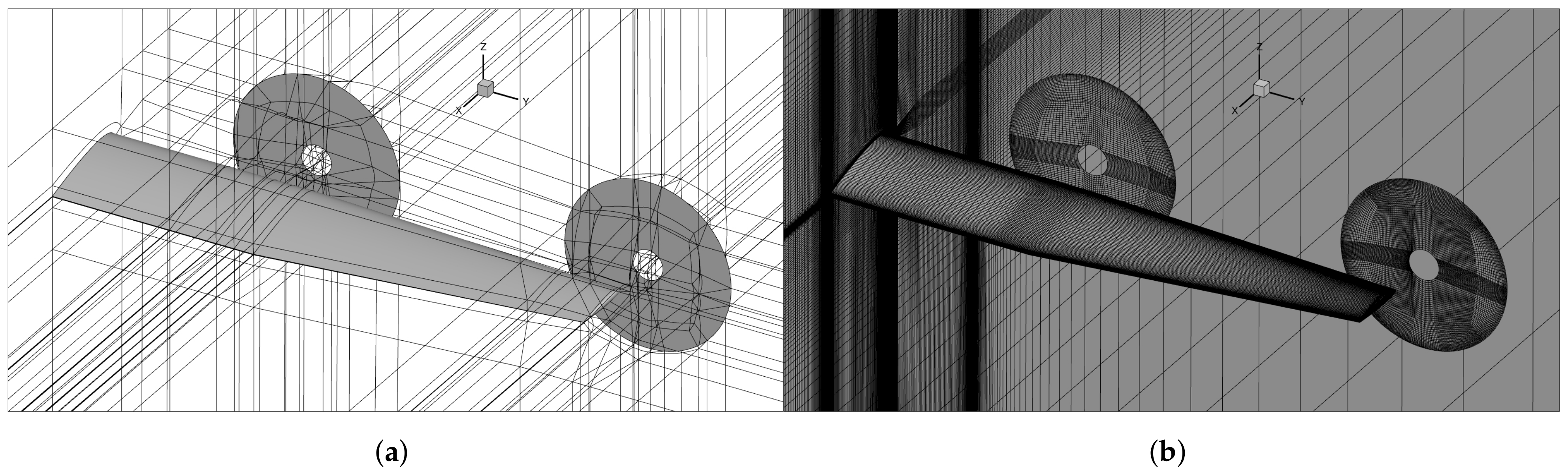
For cruise and climb CFD simulations, four different multi-block structured body-conformal hexahedral meshes were generated, sharing the same blocking topology (Figure 3a) and only differing for the tip propeller (and hub) diameter, according to the set of four values included in Table 2 and Table 3. Each of the four computational grids can be coarsened two-levels down by agglomerating two-by-two adjacent cells along each of the three block directions (obtaining medium and coarse mesh levels). This is used to speed-up initial transients of flow computations starting from scratch and to allow for multi-grid acceleration in flow simulations using CIRA ZEN solver. At the fine-mesh level (no cells agglomeration) the grid size is approximately equal to 26.6$\times {10}^6$ cells (on wing surface: 352 cells chordwise, 156 spanwise, Figure 3b), distributed in 362 structured blocks. The computational domain far-field boundary is distant 60 root chord lengths upstream of the wing, 70 downstream and 40 above and below, while the lateral domain extent is 9 times the wing half span. In choosing the computational domain size, best practices and guidelines reviewed in [28] and recommended by Hirsch [29] and Spalart and Rumsey [30] were followed, the selected far-field distance being in accordance with suggestions included in the abovementioned references on using at least 50 body lengths in the free-stream direction for 3D simulation of a wing flow.

2.7. VLM Domain Discretization

The same VLM grid of about 1800 nodes was used for all test cases, in power-off and power-on conditions. The surface discretization (Figure 4) was generated in order to take into account inboard and outboard propellers’ slipstream effects. At least 10 span-wise sections for propeller radius are needed to appreciate the slipstream effect on wing-load with sufficient accuracy.

2.8. Numerical Solutions

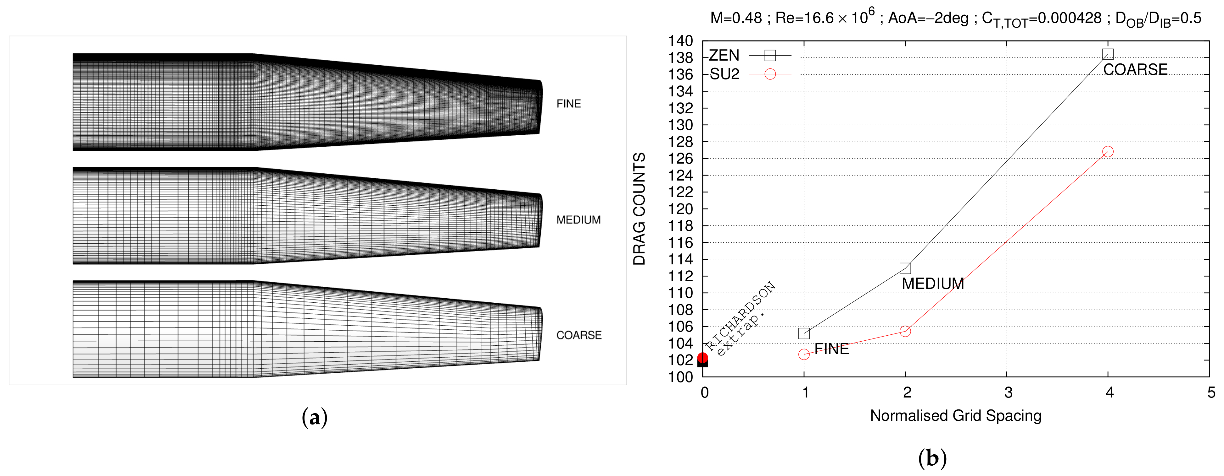
FVM results for all test cases included in Table 2 and Table 3 were obtained using CIRA ZEN solver. However, power-off and IB-OB-1 cases in cruise flight conditions were also simulated using SU2 CFD code, as described in Section 2.1. Besides providing an additional numerical estimate of aerodynamic performance at selected computed conditions, this provided input flow-fields for far-field force methods used in drag breakdown analysis, described in Section 3.2. To justify the use of the fine mesh and to obtain guidelines for further calculations, a grid convergence analysis over the three mesh levels introduced above (coarse, medium and fine) for the two different solvers is illustrated in

Table 4. Grid convergence data of CFD computations using Finite Volume Methods ($M=0.480$; $Re=16.6\times {10}^6$; IB-OB-1 test case; $AoA=-2$°).

	Grid Level 2	Computed Value 1			Order of Convergence			Richardson’s Extrapolation			Grid Convergence Index [%]			Asymptotic Range of Convergence Check
		${\mathit{C}}_{\mathit{L}}$	${\mathit{C}}_{\mathit{D}}$	${\mathit{C}}_{\mathit{M}}$	${\mathit{C}}_{\mathit{L}}$	${\mathit{C}}_{\mathit{D}}$	${\mathit{C}}_{\mathit{M}}$	${\mathit{C}}_{\mathit{L}}$	${\mathit{C}}_{\mathit{D}}$	${\mathit{C}}_{\mathit{M}}$	${\mathit{C}}_{\mathit{L}}$	${\mathit{C}}_{\mathit{D}}$	${\mathit{C}}_{\mathit{M}}$	${\mathit{C}}_{\mathit{L}}$	${\mathit{C}}_{\mathit{D}}$	${\mathit{C}}_{\mathit{M}}$
ZEN	COARSE	0.26	0.0138	−1.33	2.2	1.7	2.6	0.26	0.0102	−1.32	n/a	n/a	n/a	1.00	0.93	1.00
	MEDIUM	0.26	0.0113	−1.32							0.43	12.33	0.25
	FINE	0.26	0.0105	−1.32							0.09	4.02	0.04
SU2	COARSE	0.25	0.0127	−1.29	1.7	3.0	1.8	0.26	0.0102	−1.33	n/a	n/a	n/a	1.01	0.97	1.01
	MEDIUM	0.26	0.0105	−1.32							1.05	3.72	1.13
	FINE	0.26	0.0103	−1.33							0.31	0.49	0.31

¹ Moment pole at quarter of Mean Aerodynamic Chord. ² Number of grid cells (hexahedra): COARSE (414′986); MEDIUM (3′319′888); FINE (26′559′104).

and Figure 5, at $AoA=-2$° with both propellers operative (IB-OB-1 test-case, Table 2). The grid refinement study follows the methodology of Grid Convergence Index (GCI) first proposed in [31] and further described in [32,33,34]. As described in [35], the GCI is a measure of the percentage the computed value is away from the value of the asymptotic numerical value and indicates an error band on how far the solution is from that asymptotic value. It also indicates how much the solution would change with a further refinement of the grid. Using this method, the uncertainty of grid convergence is quantified, with reference to discretization errors of the simulation. The outcome of grid convergence analysis is reported in Table 4, where GCIs are defined for lift, drag and pitching moment coefficients, and the asymptotic range of convergence of computed solutions is assessed, checking that the values included in the last three columns of Table 4 are approximately one [35]. It is worth recalling that ZEN is a cell-centred solver, while SU2 is node-based. Therefore, using the same computational mesh as in the present case translates in an effectively different spatial discretization, in particular in the first layers of cells near solid walls, where SU2-computed skin friction values might be lower (59 d.c. compared to 62 d.c. from ZEN simulation, at fine grid level). This effect, however, vanishes as the grid spacing ideally tends towards zero.

3. Results

3.1. Drag Reduction

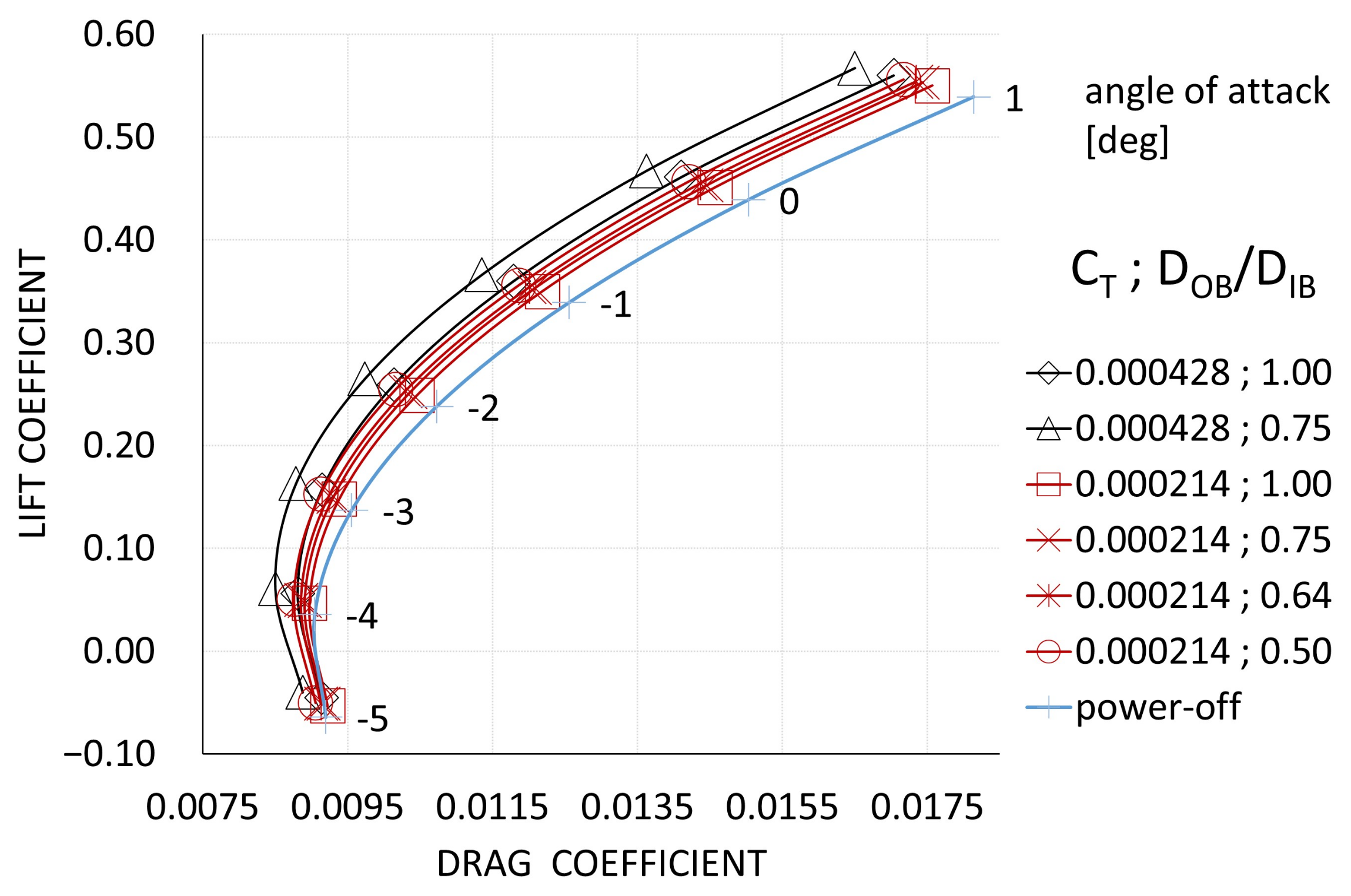
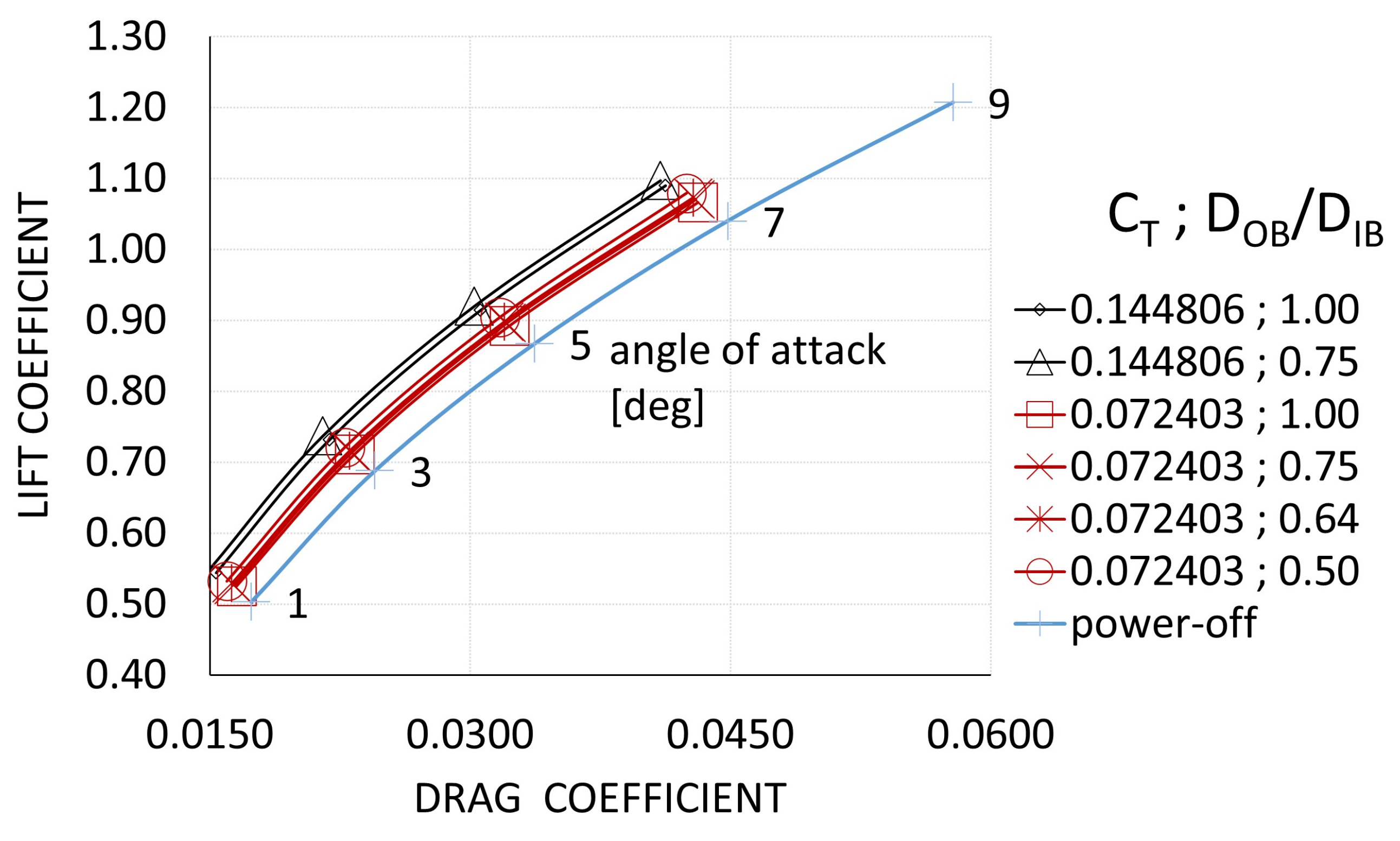
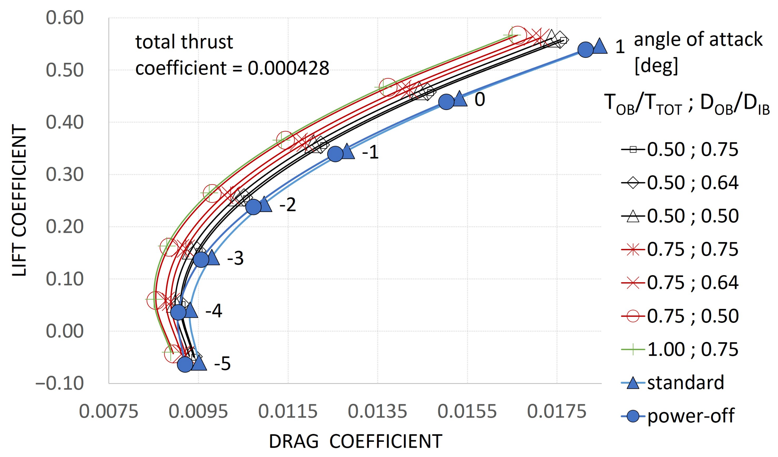
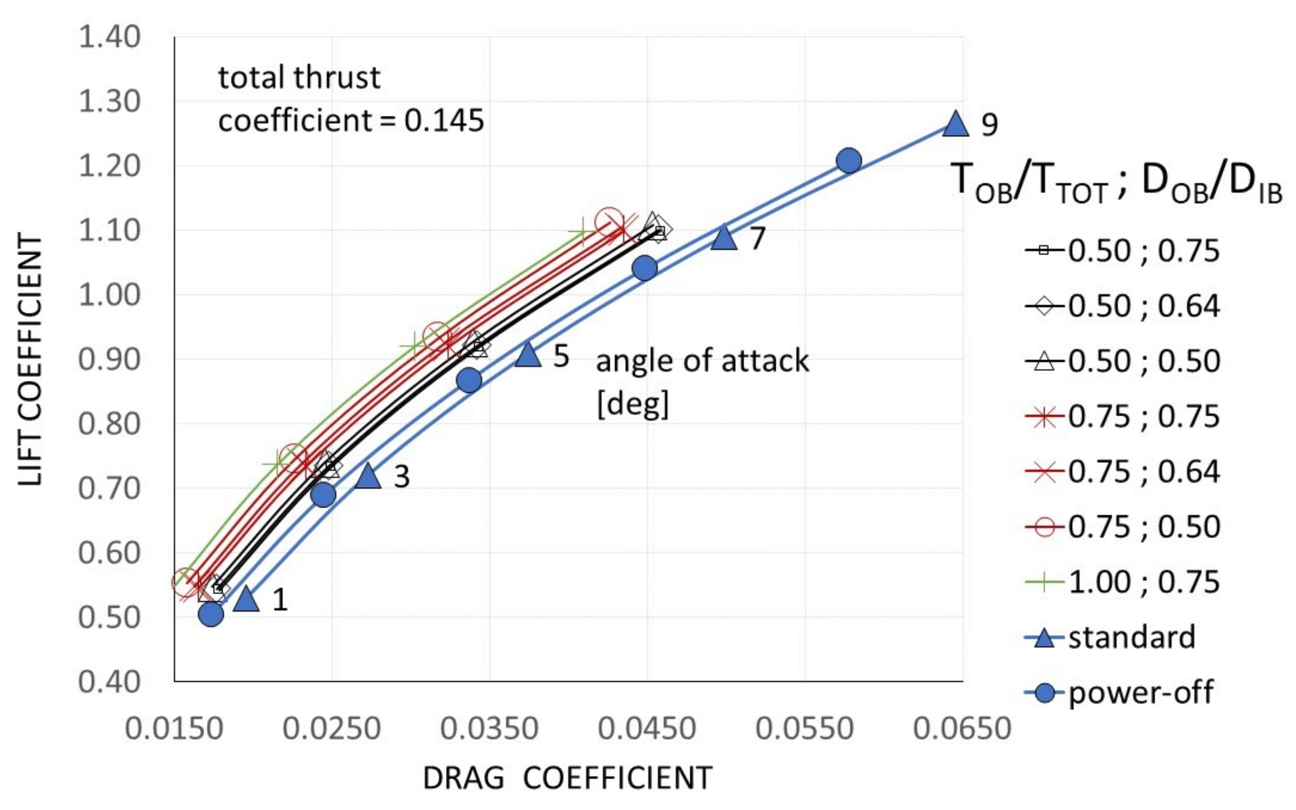
Drag polar curves computed using CIRA ZEN solver and the fine mesh level are illustrated for test cases with OB propeller only in Figure 6 and Figure 7 for cruise and climb flight conditions, respectively, and at different angles of attack, together with corresponding polar curves in power-off conditions. It is worth highlighting that the propellers’ diameter ratio ($D_{OB}/D_{IB}$) is essentially proportional to the ratio of the outboard propeller diameter over a reference wing chord length, the inboard propeller diameter being fixed in all test cases (Table 2 and Table 3). In both conditions and in almost the entire range of analyzed angles of attack, the tip propeller reduces configuration drag at constant lift with large impact for higher thrust coefficients and/or smaller diameters. Similar diagrams are included in Figure 8 and Figure 9 for the test cases with both IB and OB propellers active (at constant total thrust), compared against reference aerodynamic performance obtained in standard configuration, with total thrust provided by the inboard propeller only (STD, Table 2 and Table 3). The impact of tip propeller on drag reduction is coherently verified, with larger benefits because higher fractions of total configuration thrust are provided at the wing tip. Power-off performance is also included in Figure 8 and Figure 9 for comparison. At a constant angle of attack, the reference (standard) configuration exhibits higher drag than the wing alone (power-off). This is of course expected, although at the same time highlights how small values of tip thrust may not suffice in improving power-off wing performance unless drag penalties of the standard power arrangement are first recovered. The reference line used to quote angles of attack in Figure 6, Figure 7, Figure 8 and Figure 9 is aligned with propellers’ axes.

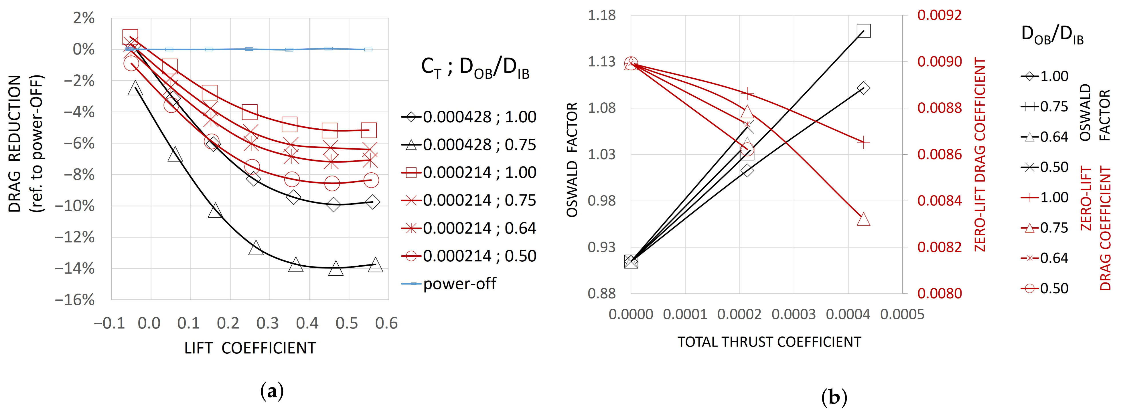
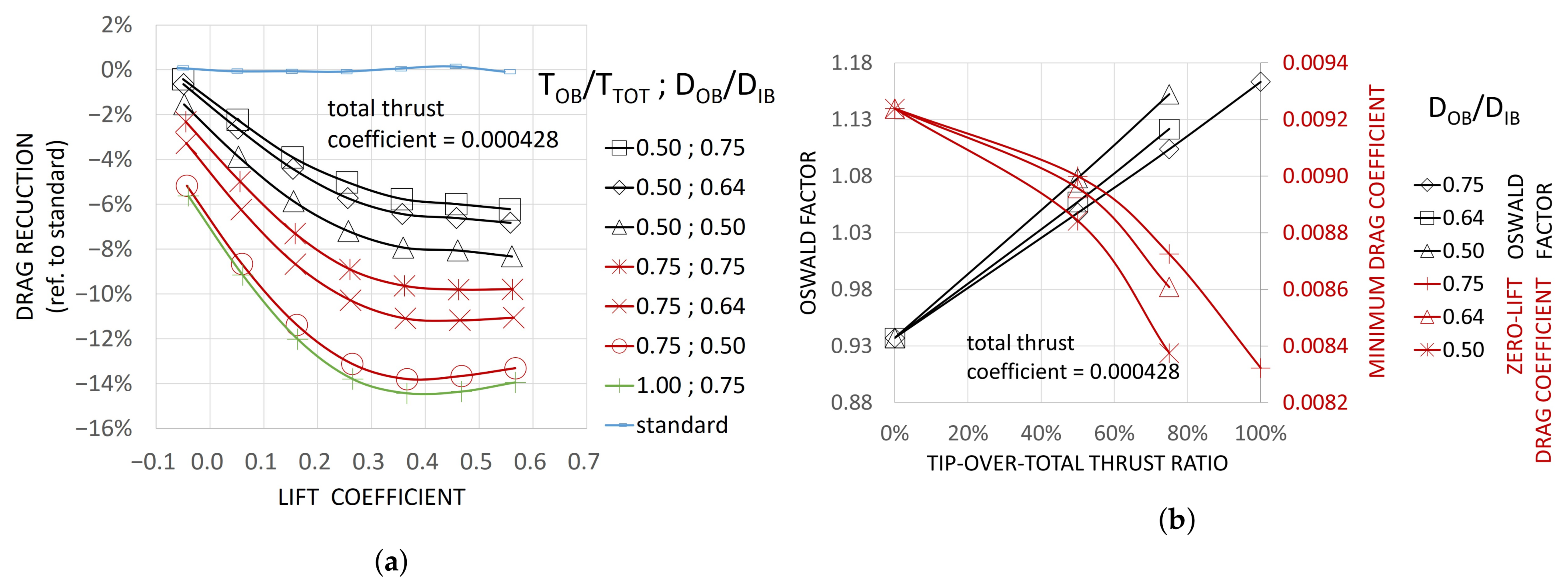
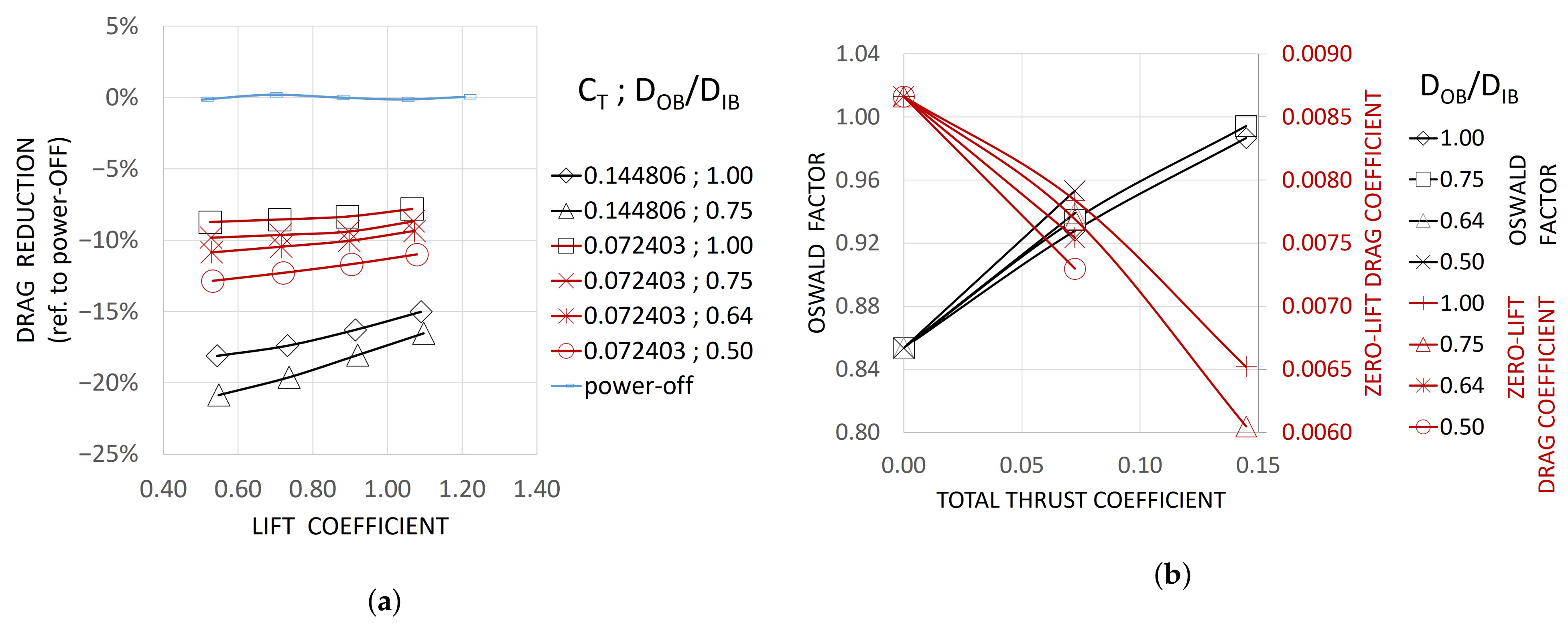
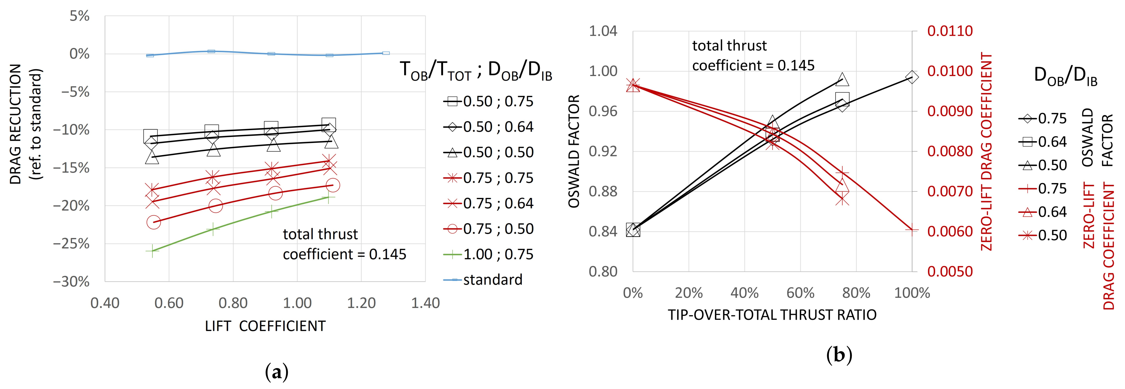
Drag reductions are evaluated assuming a three-term quadratic approximation [36] for the reference configuration (either power-off or standard) using least-squares fitting on corresponding CFD data. Then, relative drag variations of non-reference cases are provided in Figure 10a, Figure 11a, Figure 12a and Figure 13a. Analyzing both cruise and climb conditions, it is observed that with increasing lift coefficient, drag reductions achieve a minimum, suggesting that at higher angles of attack, the interaction between tip propeller slipstream and wing trailing vortices becomes weaker.

A classical two-term quadratic approximation [36] is instead used to compute the Oswald factor and zero-lift drag coefficient of all analyzed cases, as reported in Figure 10b, Figure 11b, Figure 12b and Figure 13b. They suggest an interpretation of power-on wing performance in terms of an equivalent power-off wing with lower induced drag, higher span efficiency and lower zero-lift drag, an aspect that will be further discussed in Section 4.

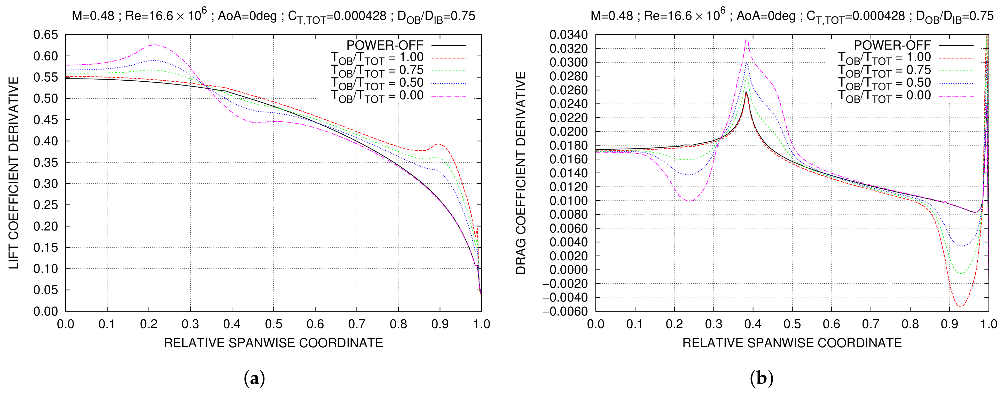
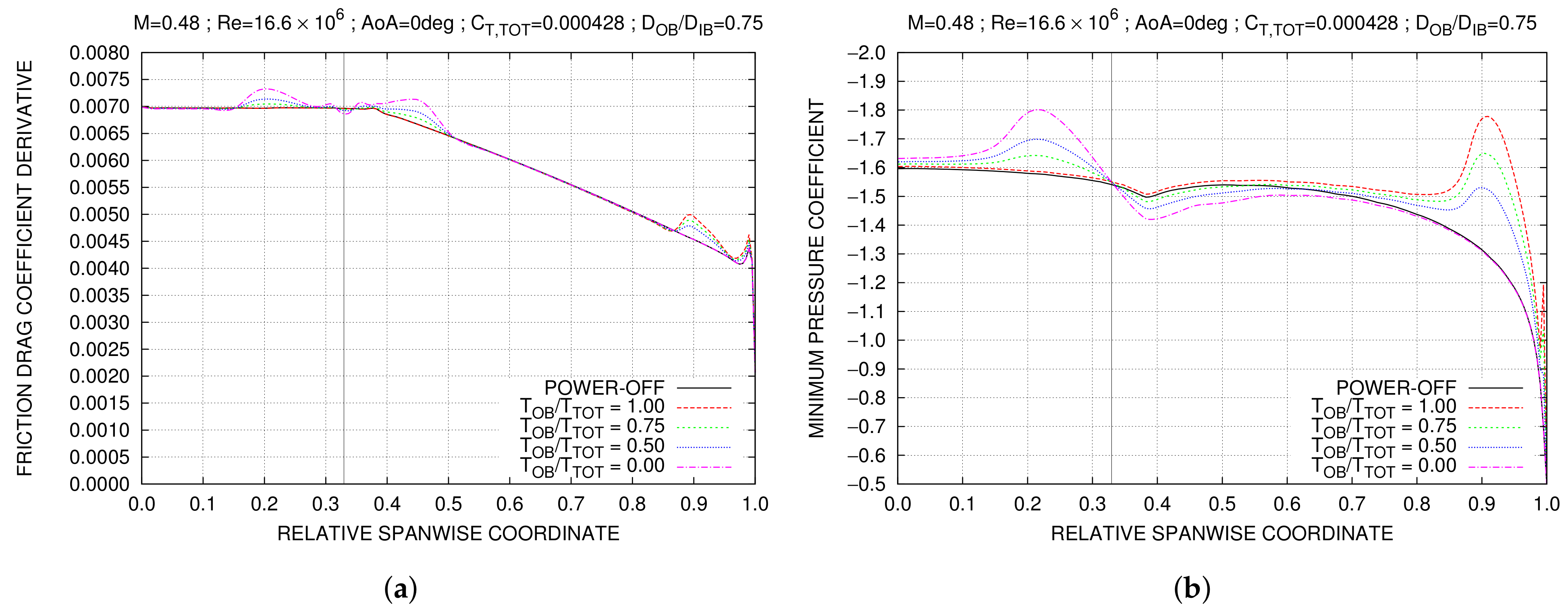
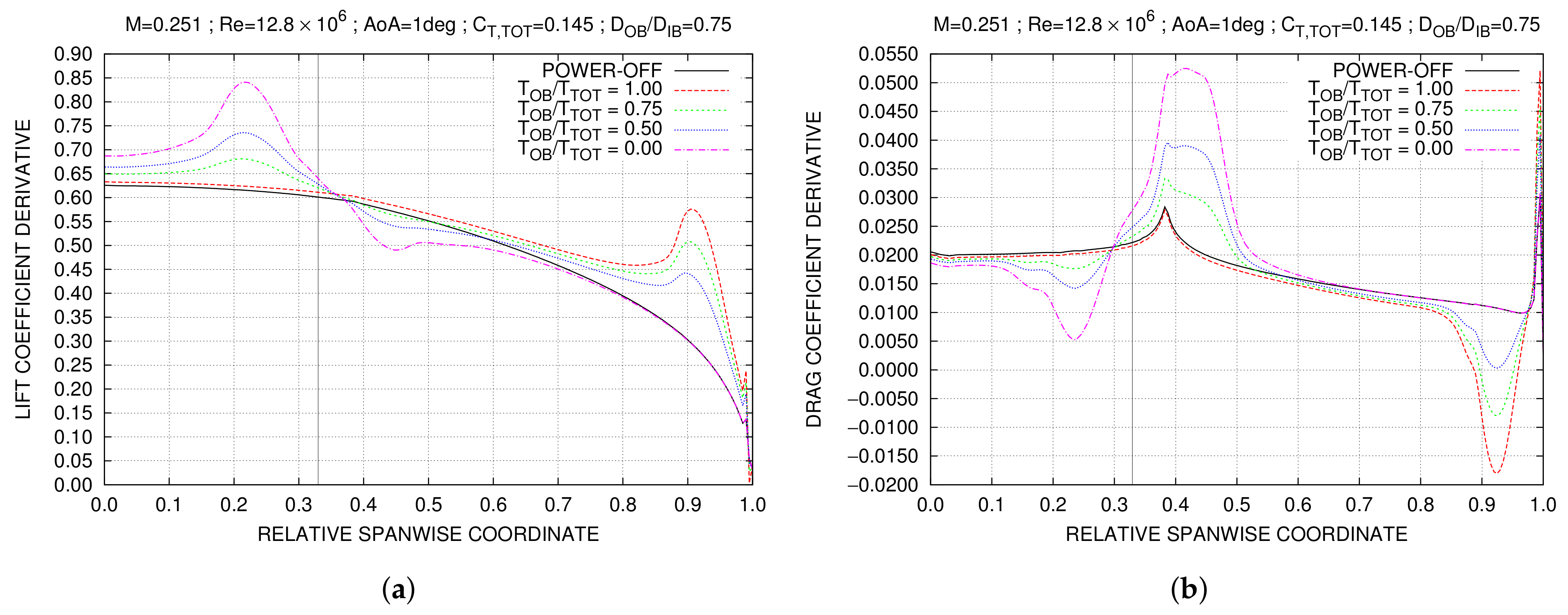
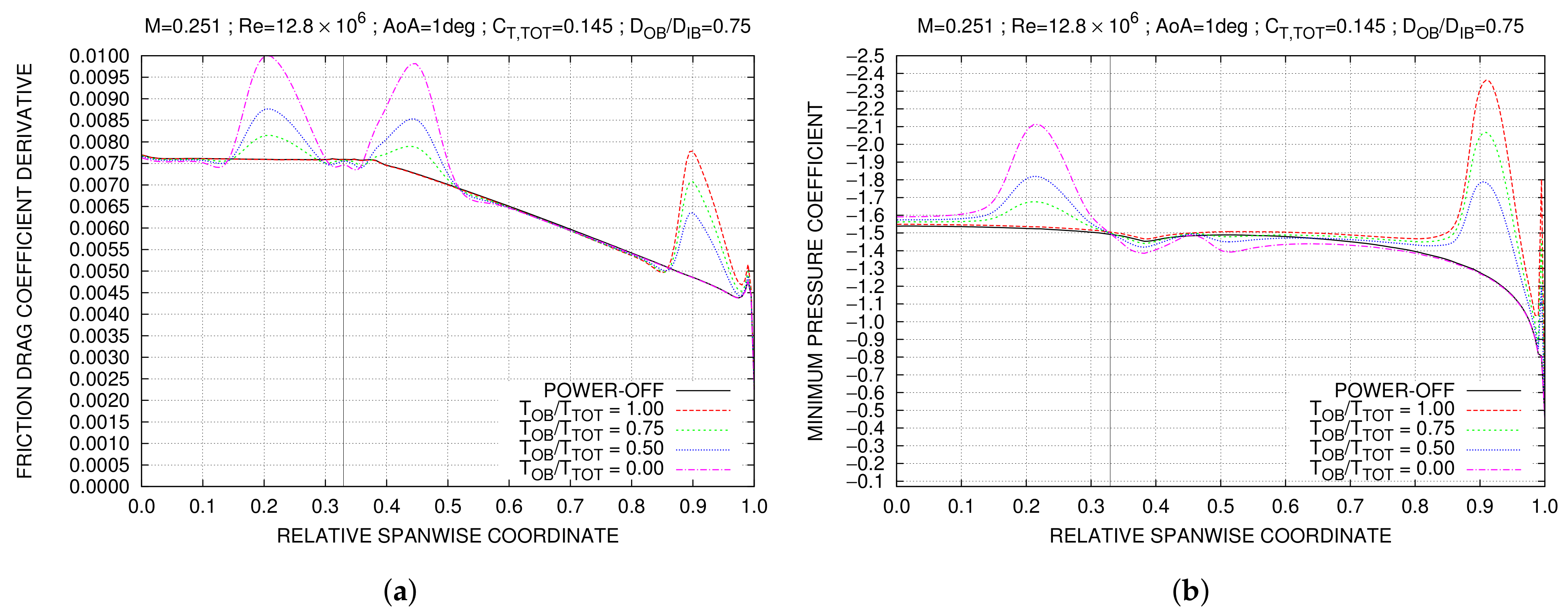
Span-wise derivatives of wing lift, total drag and friction drag, as well as distributions of minimum pressure coefficient of wing sections along the span, are illustrated in Figure 14 and Figure 15 (cruise flight) and Figure 16 and Figure 17 (climb flight), respectively, where a vertical solid line indicates the inboard propeller axis location in the spanwise direction. Derivatives of aerodynamic force coefficients are provided in symmetric form, in the sense that their integral between $[0,1]$ (instead of $[-1,1]$) provides the global force coefficient resulting from the whole (symmetric) wing load. Four different power conditions are included in spanwise loading diagrams, corresponding to different thrust distributions between IB and OB propellers, at constant total thrust coefficient. The baseline (power-off) wing loading is included for reference and outboard-over-inboard propellers diameters ratio is set at $0.75$. Wing loads are compared at a constant angle of attack ($AoA=0$° in cruise flight, $AoA=1$° in climb flight) with total lift coefficient variations of $2÷4$ counts between the different analyzed power conditions. In particular, Figure 14b, Figure 15b and Figure 16b clearly highlight how drag reductions are achieved at the wing tip, while the inboard propeller slightly increases wing drag. Higher drag derivatives are observed, for example, in correspondence with the inboard propeller axis, mainly due to the local increase in dynamic pressure, which, in turn, is also responsible for the increase in friction drag on both sides of propeller axis (Figure 15a and Figure 17a).

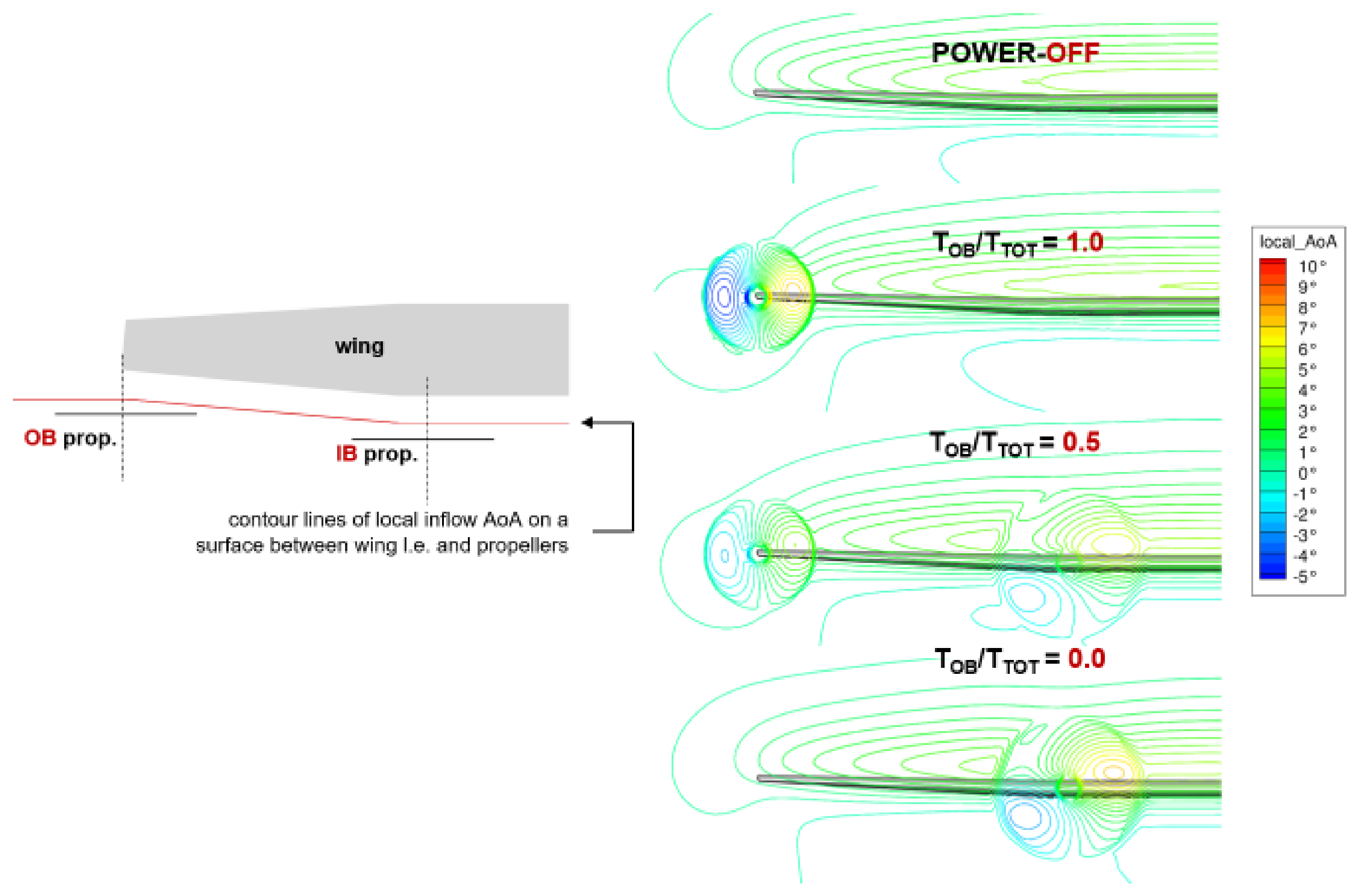
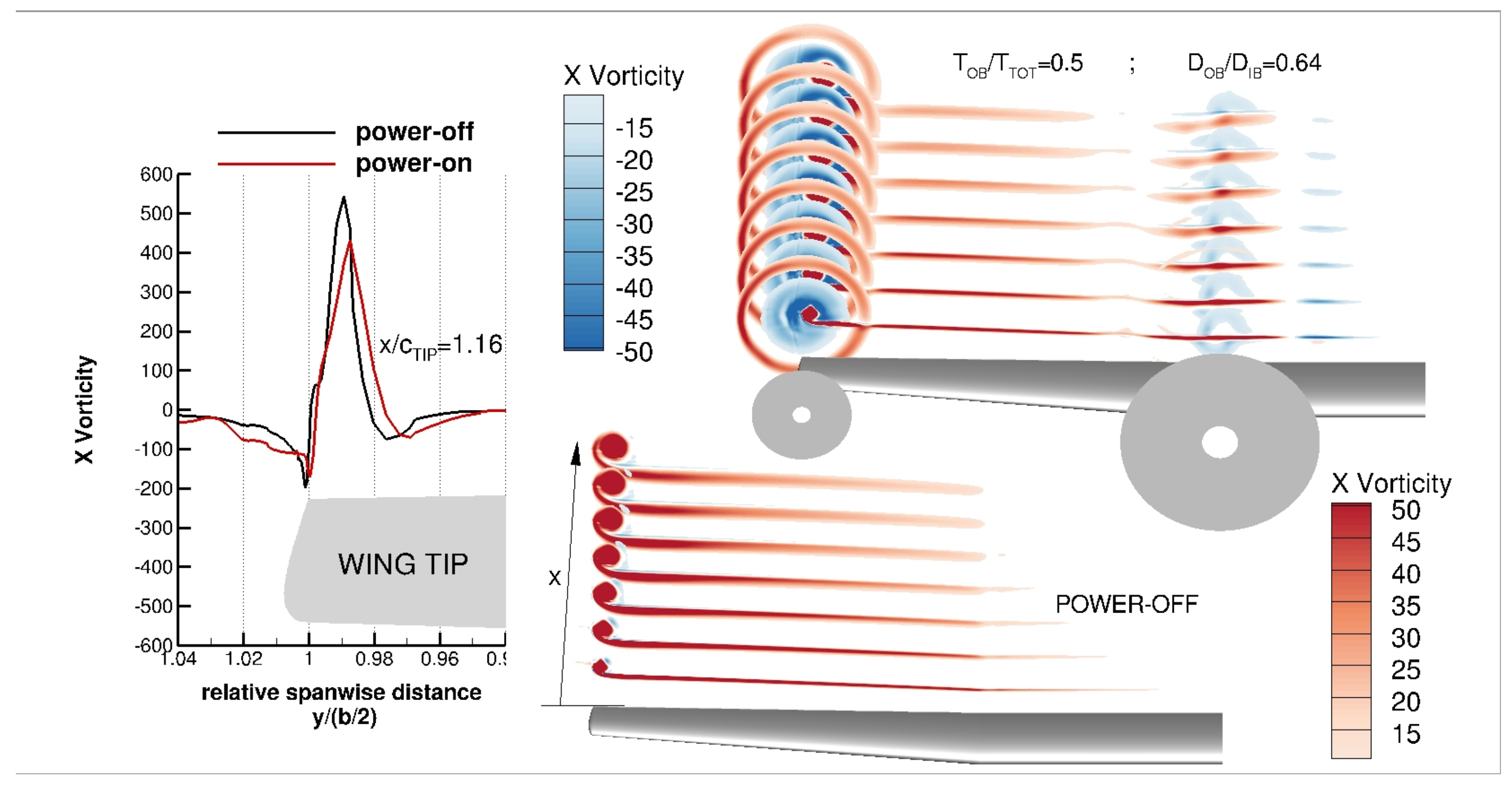
The propellers’ swirl effect is instead illustrated in Figure 18, where visualizations of local inflow angle of attack are provided on a surface located between the wing leading edge and propellers’ planes, at different thrust distributions. The impact of the OB propeller on the wing tip vortex is instead visible from Figure 19, where contour plots of stream-wise vorticity at zero angle of attack are included on several stations downstream of the wing for both power-off and one of the analyzed power-on conditions with both propellers operative, highlighting the reduction in vorticity peak at the wing tip.

3.2. Drag Breakdown

The aerodynamic force analysis has been studied by the far-field method described in Section 2.3. Both power-on (IB-OB-1) and power-off (OFF) configurations have been analyzed to confirm that the DEP can reduce the overall aerodynamic drag, modifying the aerodynamic load distribution and decreasing the induced drag.

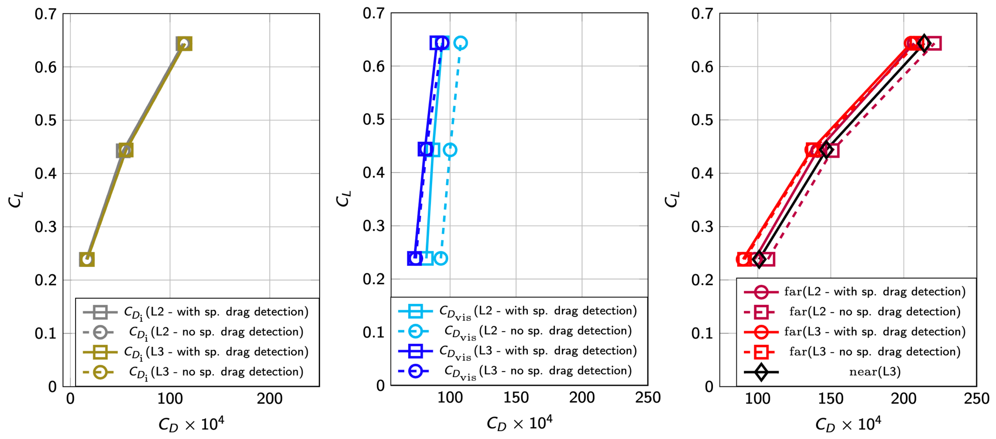
First, the method has been applied to the flow-field data obtained by SU2 and two different mesh levels (medium and fine) for the OFF configuration. As previously mentioned, far-field force analysis allows us to partially identify and remove the spurious drag contribution due to the numerical error; for each mesh level, the aerodynamic force was computed with and without spurious drag detection to assess the sensitivity of the drag breakdowns provided with respect to the spatial grid resolution.

The results obtained for the medium mesh level at AoA $=-2^{°},0^{°},2^{°}$ are collected in

Table 5. OFF configuration (medium mesh level) at $R{e}_{\infty }=16.6\times {10}^6$, $M_{\infty }=0.480$. Breakdown of the drag polars without spurious drag detection; induced drag computed by Maskell’s formula.

AoA	${\mathit{C}}_{{\mathit{D}}_{\mathbf{near}}}$	${\mathit{C}}_{{\mathit{D}}_{\mathbf{far}}}$	${\mathit{C}}_{{\mathit{D}}_{\mathbf{vis}}}$	${\mathit{C}}_{{\mathit{D}}_{\mathit{i}}}$
$-2^{°}$	107	109	93	16
$0^{°}$	151	154	100	53
$2^{°}$	221	221	108	113

(without spurious drag detection) and

Table 6. OFF configuration (medium mesh level) at $R{e}_{\infty }=16.6\times {10}^6$, $M_{\infty }=0.480$. Breakdown of the drag polars with spurious drag detection; induced drag computed by Maskell’s formula.

AoA	${\mathit{C}}_{{\mathit{D}}_{\mathbf{near}}}$	${\mathit{C}}_{{\mathit{D}}_{\mathbf{far}}}$	${\mathit{C}}_{{\mathit{D}}_{\mathbf{vis}}}$	${\mathit{C}}_{{\mathit{D}}_{\mathit{i}}}$	${\mathit{C}}_{{\mathit{D}}_{\mathbf{sp}}}$
$-2^{°}$	107	98	82	16	11
$0^{°}$	151	141	87	53	13
$2^{°}$	221	207	94	113	14

(with spurious drag detection) in terms of near-field drag coefficient $C_{D_{\mathrm{near}}}$, far-field drag coefficient $C_{D_{\mathrm{far}}}$, viscous drag coefficient $C_{D_{\mathrm{vis}}}$ induced drag coefficient $C_{D_{\mathrm{i}}}$ and spurious drag coefficient $C_{D_{\mathrm{sp}}}$. Similarly, the results obtained for the fine mesh are collected in

Table 7. OFF configuration (fine mesh level) at $R{e}_{\infty }=16.6\times {10}^6$, $M_{\infty }=0.480$. Breakdown of the drag polars without spurious drag detection; induced drag computed by Maskell’s formula.

AoA	${\mathit{C}}_{{\mathit{D}}_{\mathbf{near}}}$	${\mathit{C}}_{{\mathit{D}}_{\mathbf{far}}}$	${\mathit{C}}_{{\mathit{D}}_{\mathbf{vis}}}$	${\mathit{C}}_{{\mathit{D}}_{\mathit{i}}}$
$-2^{°}$	101	91	74	17
$0^{°}$	147	138	82	56
$2^{°}$	214	209	94	115

(without spurious drag detection) and

Table 8. OFF configuration (fine mesh level) at $R{e}_{\infty }=16.6\times {10}^6$, $M_{\infty }=0.480$. Breakdown of the drag polars with spurious drag detection; induced drag computed by Maskell’s formula.

AoA	${\mathit{C}}_{{\mathit{D}}_{\mathbf{near}}}$	${\mathit{C}}_{{\mathit{D}}_{\mathbf{far}}}$	${\mathit{C}}_{{\mathit{D}}_{\mathbf{vis}}}$	${\mathit{C}}_{{\mathit{D}}_{\mathit{i}}}$	${\mathit{C}}_{{\mathit{D}}_{\mathbf{sp}}}$
$-2^{°}$	101	90	73	17	1
$0^{°}$	147	137	81	56	1
$2^{°}$	214	205	90	115	4

(with spurious drag detection).

The main outcomes of the gird sensitivity analysis are shown in Figure 20 and here summarized:

• The far-field total drag obtained using the medium mesh level with a proper spurious drag detection allows us to reach the same near-field drag of the fine mesh level.
• No relevant difference can be found applying the far-field method with and without spurious drag detection on the fine mesh level; on this grid level, the spurious drag is therefore negligible.
• The induced drag contribution, computed by Maskell’s formula, is not affected by the spurious drag detection (as expected), but is slightly affected by the mesh level thanks to an improved resolution of the free vortices in the wing wake.

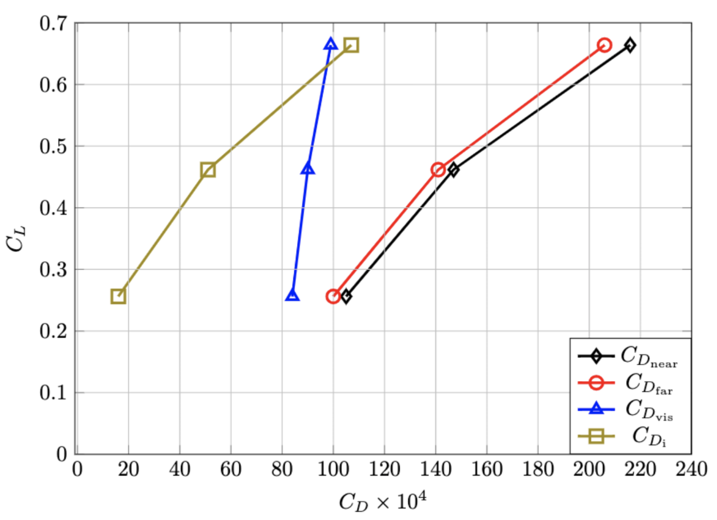
Since sufficiently accurate results have been obtained with the medium mesh level properly removing the spurious drag contribution with lower computational effort, the aerodynamic drag breakdown for the IB-OB-1 configuration was performed on this mesh level. The results are shown in Figure 21 and

Table 9. IB-OB-1 configuration at $R{e}_{\infty }=16.6\times {10}^6$, $M_{\infty }=0.480$. Drag breakdown with spurious drag detection on medium mesh levels; induced drag computed by Maskell’s formula.

AoA	${\mathit{C}}_{{\mathit{D}}_{\mathbf{near}}}$	${\mathit{C}}_{{\mathit{D}}_{\mathbf{far}}}$	${\mathit{C}}_{{\mathit{D}}_{\mathbf{vis}}}$	${\mathit{C}}_{{\mathit{D}}_{\mathit{i}}}$
$-2^{°}$	105	100	84	16
$0^{°}$	147	141	90	51
$2^{°}$	216	206	99	107

for AoA $=-2^{°},0^{°},2^{°}$.

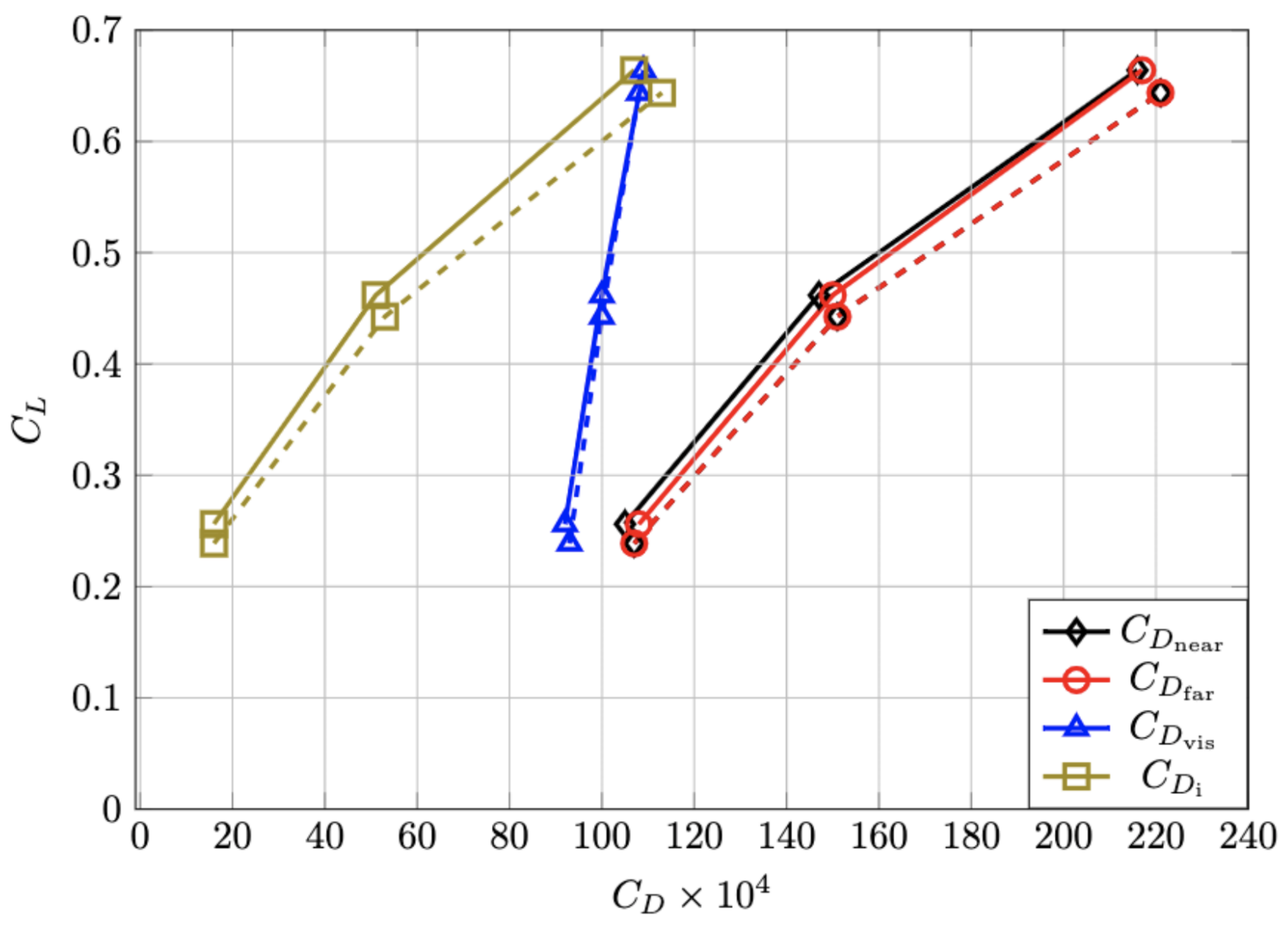
The comparison between the two configurations is presented in

Table 10. Comparison between IB-OB-1 and OFF configurations at $R{e}_{\infty }=16.6\times {10}^6$, $M_{\infty }=0.480$. Breakdown of the drag polars with spurious drag detection; induced drag computed by Maskell’s formula.

$\mathit{\alpha }$	$\mathsf{\Delta }{\mathit{C}}_{{\mathit{L}}_{\mathbf{near}}}$	$\mathsf{\Delta }{\mathit{C}}_{{\mathit{D}}_{\mathbf{near}}}$	$\mathsf{\Delta }{\mathit{C}}_{{\mathit{D}}_{\mathbf{far}}}$	$\mathsf{\Delta }{\mathit{C}}_{{\mathit{D}}_{\mathbf{vis}}}$	$\mathsf{\Delta }{\mathit{C}}_{{\mathit{D}}_{\mathit{i}}}$
$-2^{°}$	0.0173	−2	+1	+1	0
$0^{°}$	0.0192	−4	−1	+1	−2
$2^{°}$	0.0203	−5	−4	+2	−6

in terms of aerodynamic coefficients variations:

$$\mathsf{\Delta }{C}_{{\mathrm{x}}_{\mathrm{y}}}=C_{{\mathrm{x}}_{\mathrm{y}}}^{\mathrm{IB}-\mathrm{OB}-1}-C_{{\mathrm{x}}_{\mathrm{y}}}^{\mathrm{OFF}}$$

(6)

whereas the drag polars are compared in Figure 22.

In addition, the far-field analysis confirms the potential benefit of DEP configurations: they improve the lift performance and decrease the overall drag. In particular, the analysis highlighted that the propeller installation slightly increases the viscous drag contribution due to the higher dynamic pressure, but further decreases the induced drag component, realizing an overall drag reduction. As the lift coefficient increases, the induced drag reduction grows, whereas the viscous drag is almost the same: the higher the lift, the higher the drag reduction obtained by the IB-OB-1 configuration.

The drag changes due to the propeller installation are even more evident when the OFF and IB-OB-1 configurations are compared at the same lift;

Table 11. Comparison between IB-OB-1 and OFF configurations at $R{e}_{\infty }=16.6\times {10}^6$, $M_{\infty }=0.480$ and same lift. Breakdown of the drag polars with spurious drag detection; induced drag computed by Maskell’s formula.

${\mathit{C}}_{\mathit{L}}$	$\mathsf{\Delta }{\mathit{C}}_{{\mathit{D}}_{\mathbf{near}}}$	$\mathsf{\Delta }{\mathit{C}}_{{\mathit{D}}_{\mathbf{far}}}$	$\mathsf{\Delta }{\mathit{C}}_{{\mathit{D}}_{\mathbf{vis}}}$	$\mathsf{\Delta }{\mathit{C}}_{{\mathit{D}}_{\mathit{i}}}$
$0.25$	−5	−2	+1	−3
$0.45$	−10	−6	0	−6
$0.65$	−14	−11	+1	−12

contains this analysis obtained with a second-order interpolation of the test points. With this interpolation, an increase in the span efficiency (Oswald’s factor) of $12\%$ was found.

3.3. Comparison with Lower-Fidelity Methodology

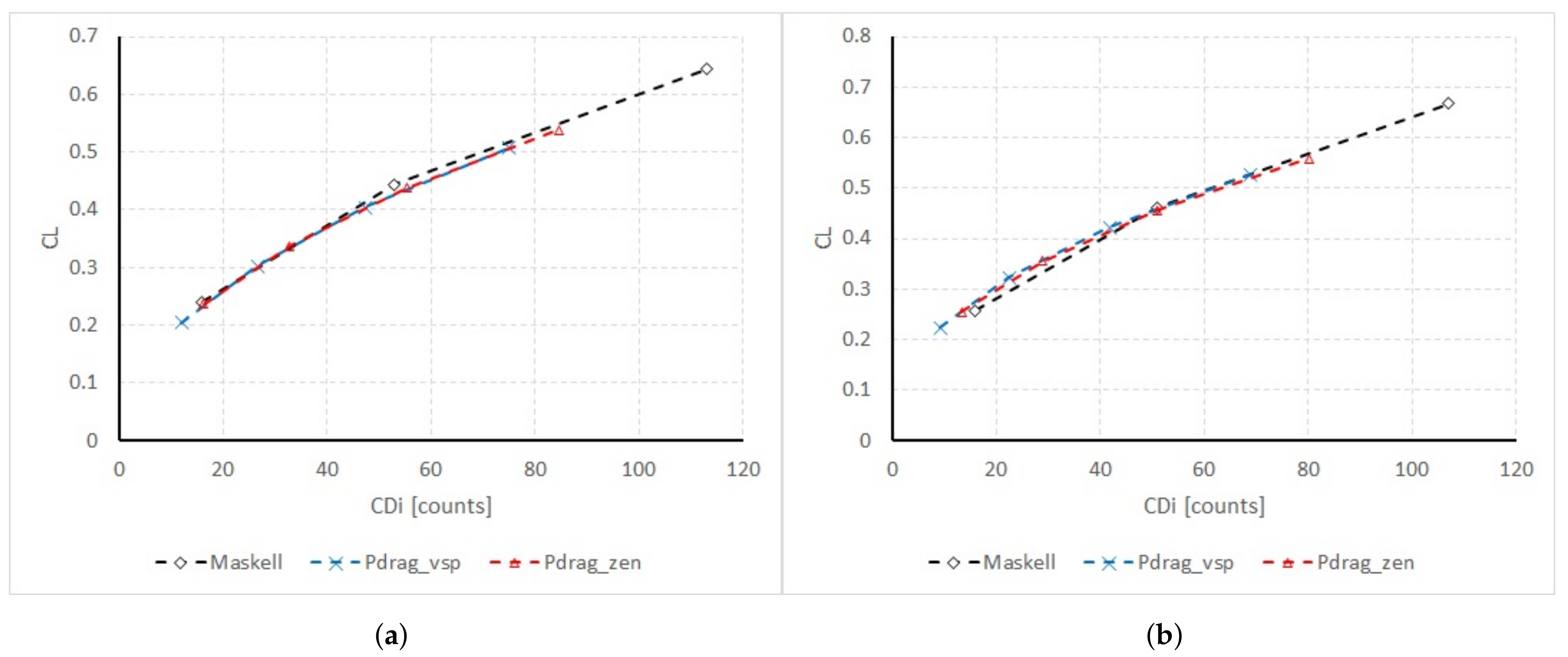
By using the approach introduced in Section 2.2, the induced drag for OFF and IB-OB-1 conditions has been estimated and compared with the results from Maskell’s formula reported in Table 8 and Table 9. As stated in Section 2.2, the procedure to evaluate the induced drag needs, as input, spanwise load distributions that can be provided from different solvers. In this simulation, spanwise loads from Vspaero [22] and CIRA ZEN [17] solvers were used. In Figure 23, a spanwise load distributions’ comparison between the output from those two different solvers is shown for the IB-OB-1 configuration, in conditions similar to $CL=0.5$. In Figure 24, the comparison, in terms of induced drag, between the different approaches used in this work is presented. The Maskell’s formula prediction is plotted in black, the Vspaero in light blue and CIRA ZEN in red. The proposed comparison highlights a good agreement between the different approaches used in this work to estimate induced drag. It is important to outline that the data matching is particularly good and close to the cruise condition ($CL\approx 0.5$).

3.4. Tip Propeller vs. Tip Winglet Drag Reduction

3.4.1. Equivalent Winglet Design

The main goal of the proposed winglet design is to understand if it is possible to replace a tip propeller characterized by $D_{OB}/D_{IB}=0.75$ and $T_{OB}/T_{TOT}=0.5$ (case IB-OB-2 in Table 2) with a winglet of reasonable dimensions. The design point is cruise condition ($M=0.480$;$Re=16.6\times {10}^6$;$C_L=0.5$) and a maximum winglet height of ≈$10\%$ of the semi-span with maximum wing footprint of +5% are assumed as geometrical constrains. To execute a full aerodynamic optimization with acceptable computational cost, an optimization chain which involves a low-fidelity aerodynamic solver, able to consider viscous effects, was used. The chain consists of an optimization tool (GAW) based on the Pareto dominance [37,38], the aerodynamic home-built low-fidelity solver Xavl [39,40] based on the open-source software AVL [41], and a post-processor. The same approach was successfully used in the Scavir project [42], where the low-fidelity results showed a good agreement with the high-fidelity ones. The winglet planform geometry was parametrized using five design sections (Figure 25a). In each station, the GAW optimization tool is allowed to modify the sweep angle, the twist angle, the chord extension and the cant angle. The overall winglet height is not a direct design variable, but the GAW tool can modify the spanwise distance between each of the five design sections. The final winglet design (Figure 25b) has an overall height equal to $10.97\%$ of the wing half-span and a cant angle of $87.7°$.

3.4.2. Drag-Reduction Comparison

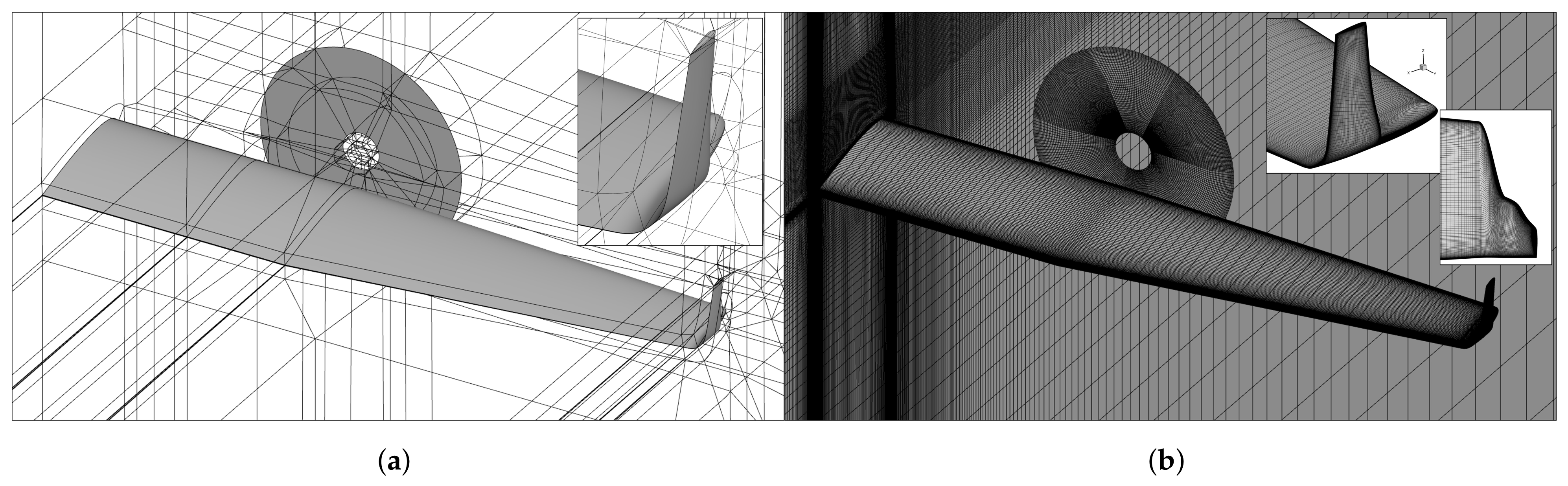
A comparison of the aerodynamic performance achieved by equipping the reference wing configuration with either a tip propeller or a tip winglet (with optimized design as described above) is herein illustrated, focusing on cruise flight conditions and constant total thrust coefficient. The selected configuration with the tip propeller is IB-OB-2 (Table 2), which provided the smallest drag reduction at a constant lift coefficient compared to the other analyzed total thrust arrangements (Figure 11a). Numerical FVM results using CIRA ZEN solver and a computational grid modified in the region of the wing tip (Figure 26b) are included in Figure 27, where aerodynamic performances of the standard reference wing/propeller configuration are compared to those obtained using either the optimized tip winglet or a tip propeller, which takes over half of total configuration thrust. Both solutions provided similar benefits at typical design lift coefficients in cruise flight conditions ($C_L\approx 0.5$). However, the different pitching moment behaviour of the two tip solutions (Figure 27b) suggests that higher tail loads might be necessary to trim the configuration in the case of a winglet installation and down-lifting horizontal tail in standard cruise conditions, with penalties on trim drag. The same approach described in previous document sections and based on three-term or two-term quadratic approximations of computed drag polars is used to compare drag reductions, Oswald’s factors and zero-lift drag coefficients in Figure 28. Filled symbols are used in Figure 28b (tip propeller curves) to highlight the thrust arrangement compared against the tip winglet configuration in Figure 27a ($T_{OB}/T_{TOT}=50$%).

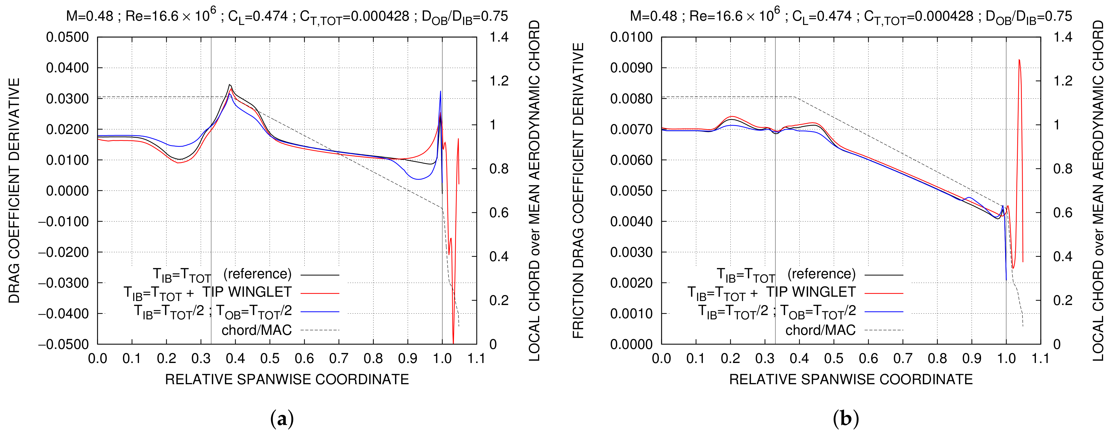
Wing spanwise loading for the three analyzed configurations are compared in Figure 29 and Figure 30, where local chord distribution is also included in all plots. Wing loads are computed at zero angle of attack for the configuration with tip winglet, while for the other two configurations, a linear interpolation on lift is performed based on computed wing loads at $AoA=0$° and $AoA=1$°, to obtain spanwise derivatives with the same lift coefficient ($C_L=0.474$). Compared to the power-off configuration, the drag contribution of the wing outermost sections is reduced by tip-propeller interactions (as already observed in the previous paragraphs), while it is increased in the configuration with the tip winglet installed, an effect which is of course globally overcome by drag reductions realized on the winglet surface itself (Figure 30). Spanwise distributions of minimum and maximum pressure at wing sections are illustrated in Figure 31, with minimum pressure plots highlighting swirl effects of the propeller slipstream (variation of local effective angle of attack) and maximum pressure (pressure at attachment line), indicating variations in local dynamic pressure due to the propellers’ blowing.

4. Discussion

Power-on configurations exhibit slightly higher lift values at a constant angle of attack compared to power-off wing performance (Figure 6, Figure 7, Figure 8 and Figure 9) as a consequence of the increased dynamic pressure (downstream of both IB and OB propellers) and effective angles of attack (due to tip propeller up-wash) at the outermost wing sections affected by tip propeller slipstream (Figure 14a and Figure 16a). Drag reductions at positive lift increase with wing lift coefficient up to an extremum (Figure 10a and Figure 11a, cruise flight conditions), then decrease at higher lift coefficients, as observed in Figure 12a and Figure 13a at climb flight conditions. They are realized at wing outboard sections (Figure 14b and Figure 16b) as a consequence of tip propeller-induced up-wash, which is opposed to wing self-induced down-wash occurring when positive lift is generated, re-orienting local forces in the direction of reducing drag components. This effect is higher as tip propeller load is increased, i.e., increasing tip thrust (at constant tip diameter) or reducing tip propeller diameter (at constant tip thrust). The Oswald’s factor estimated with a two-term quadratic approximation of the drag polar curve also increases with tip propeller load (Figure 10b, Figure 11b, Figure 12b and Figure 13b), suggesting an interpretation of power-on wing performance in terms of an equivalent power-off wing with lower induced drag and higher span efficiency. This equivalent wing is also characterized by a lower zero-lift drag. While this might not be straightforward or expected, as both propellers increase friction drag in slipstream regions (Figure 15a and Figure 17a), it is a consequence of the different wing loadings at zero-lift conditions with or without tip propeller effects, resulting in different pressure drag distributions. Indeed, wing-induced drag at a global zero lift coefficient is generally non-zero (due to a locally non-zero spanwise lift distribution), and is modified by propellers’ interactions. The effect of the inboard propeller is observed comparing standard and reference test cases’ polar curves (Figure 8 and Figure 9) and spanwise loading (Figure 14b and Figure 16b). While swirl effects almost compensate on left and right sides of the propeller slipstream, the increased dynamic pressure ratio (local over free-stream) experienced by wing sections affected by propeller wake results in a higher magnitude of force derivatives in the spanwise direction (Figure 14b and Figure 16b), which corresponds to higher global lift and drag coefficients compared to power-off conditions (Figure 8 and Figure 9).

The far-field force analysis confirms potential benefits of tip propeller installations, improving lift performance and decreasing the overall drag. A slight increase in the viscous drag contribution, due to the higher dynamic pressure, is overwhelmed by a larger decreases in the induced drag component, resulting in an overall drag reduction. As the lift coefficient increases, the induced drag reduction increases as well, whereas viscous drag is almost the same (Figure 22).

Comparing drag characteristics of the standard reference configuration against those obtained for the configuration equipped with either a tip winglet or a tip propeller (at constant total thrust, Figure 27a), both solutions provided similar benefits at typical design lift coefficients in cruise flight conditions ($C_L\approx 0.5$), the comparison involving an optimized winglet design and the worst performing IB-OB thrust arrangement among those analyzed in Figure 11a. However, the difference in pitching moment coefficients of the two tip solutions (Figure 27b) suggests that higher tail loads might be required to trim the configuration in the case of a winglet installation and down-lifting horizontal tail in standard cruise conditions, resulting in higher trim drag. The tip winglet is less effective than a tip propeller installation on reducing configuration drag at lower lift coefficients (Figure 27a and Figure 28a), increasing reference configuration drag in approximately half of the analyzed lift coefficients’ range, where a tip propeller is instead providing drag reductions (Figure 28a). This is also highlighted using a two-term quadratic approximation of the drag polar curve, providing a higher Oswald’s factor compared to selected IB-OB propellers’ configuration, but with a higher zero-lift drag coefficient as a consequence of the increased wet area and associated friction drag.

This article focused on aerodynamic aspects only of tip propeller installations and engine nacelles were not taken into account (although, inoperative propeller regions near hubs were considered). Nevertheless, other aspects of aircraft design come into discussion. For example, maneuverability and controllability issues are foreseen, considering that minimum pressure coefficients observed at the wing tip are lower when the tip propeller is operative (Figure 15b and Figure 17b), as a consequence of the increased effective angles of attack at the outermost wing sections. Tip propeller installations might therefore be critical from a safety point of view at higher incidence angles, as the stall pattern could be significantly modified.

5. Conclusions

The possibility to reduce lift-induced drag by a proper installation of wing-tip propellers has been investigated in the present paper. In particular, a regional-aircraft-like straight wing in a subsonic regime has been studied with a distributed propulsion consisting of two inboard and two outboard propellers.

The main results of this study can be summarized as follows:

• The reduction in intensity of wing-tip vortices, thanks to the adoption of tip propellers, introducing a swirl opposite to the one induced by tip vortices, has been confirmed (Figure 19). The equivalent wing span efficiency is therefore increased.
• A significant reduction in the total wing drag was obtained. The estimated reduction is ≈$6\%$ (≈$10\%$) at typical cruise (climb) flight conditions, assuming wingtip-mounted propellers taking over half of the total thrust usually provided by turbo-prop engines installed at the inboard wing position.
• Tip propellers modify wing spanwise loading, reducing wing-induced drag even at a zero global lift coefficient. Therefore, the equivalent wing drag at zero lift is lower, despite the increase in skin friction at wing sections immersed in the propellers’ slipstream (Figure 10b, Figure 11b, Figure 12b and Figure 13b).
• The adoption of a far-field drag analysis allowed us to identify both lift-induced and viscous drag contributions. The dominance of lift-induced drag reduction against viscous drag increase is confirmed. As the lift coefficient increases, the induced drag reduction increases as well. (Figure 22).
• A tip winglet installation can be competitive in terms of aerodynamic performance improvements against a standard tip winglet installation (Figure 27 and Figure 28), with different impacts on wing pitching moment and larger drag reductions at moderate lift coefficients.

References

- Friedrich, C.; Robertson, P. Hybrid-Electric Propulsion for Aircraft. J. Aircr. 2015, 52, 176–189. [Google Scholar] [CrossRef]
- Moore, M.D. Misconceptions of Electric Aircraft and their Emerging Aviation Markets. In Proceedings of the 52nd Aerospace Sciences Meeting, National Harbor, MD, USA, 13–17 January 2014. [Google Scholar] [CrossRef]
- Sinnige, T.; van Arnhem, N.; Stokkermans, T.C.A.; Eitelberg, G.; Veldhuis, L.L.M. Wingtip-Mounted Propellers: Aerodynamic Analysis of Interaction Effects and Comparison with Conventional Layout. J. Aircr. 2019, 56, 295–312. [Google Scholar] [CrossRef] [Green Version]
- Snyder, M.H.; Zumwalt, G.W. Effects of wingtip-mounted propellers on wing lift and induced drag. J. Aircr. 1969, 6, 392–397. [Google Scholar] [CrossRef]
- Patterson, J.C.J.; Bartlett, G.R. Evaluation of Installed Performance of a Wing-Tip-Mounted Pusher Turboprop on a Semispan Wing; Technical Report; NASA: Washington, DC, USA, 1987. [Google Scholar]
- Loth, J.; Loth, F. Induced drag reduction with wing tip mounted propellers. In Proceedings of the 2nd Applied Aerodynamics Conference, Seattle, WA, USA, 21–23 August 2012. [Google Scholar] [CrossRef]
- De Vries, R.; van Arnhem, N.; Sinnige, T.; Vos, R.; Veldhuis, L.L. Aerodynamic interaction between propellers of a distributed-propulsion system in forward flight. Aerosp. Sci. Technol. 2021, 118, 107009. [Google Scholar] [CrossRef]
- Fratello, G.; Favier, D.; Maresca, C. Experimental and numerical study of the propeller/fixed wing interaction. J. Aircr. 1991, 28, 365–373. [Google Scholar] [CrossRef]
- Miranda, L.; Brennan, J. Aerodynamic effects of wingtip-mounted propellers and turbines. In Proceedings of the 4th Applied Aerodynamics Conference, San Diego, CA, USA, 9–11 June 2012. [Google Scholar] [CrossRef]
- Janus, J.M.; Chatterjee, A.; Cave, C. Computational analysis of a wingtip-mounted pusher turboprop. J. Aircr. 1996, 33, 441–444. [Google Scholar] [CrossRef]
- Vecchia, P.D.; Malgieri, D.; Nicolosi, F.; De Marco, A. Numerical analysis of propeller effects on wing aerodynamic: Tip mounted and distributed propulsion. Transp. Res. Procedia 2018, 29, 106–115. [Google Scholar] [CrossRef]
- Stoll, A.M.; Bevirt, J.; Moore, M.D.; Fredericks, W.J.; Borer, N.K. Drag Reduction Through Distributed Electric Propulsion. In Proceedings of the 14th AIAA Aviation Technology, Integration, and Operations Conference, Atlanta, GA, USA, 16–20 June 2014. [Google Scholar] [CrossRef] [Green Version]
- Menter, F.R. Two-equation eddy-viscosity turbulence models for engineering applications. AIAA J. 1994, 32, 1598–1605. [Google Scholar] [CrossRef] [Green Version]
- Ferraro, D.; Lauria, A.; Penna, N.; Gaudio, R. Temporal development of unconfined propeller scour in waterways. Phys. Fluids 2021, 33, 095119. [Google Scholar] [CrossRef]
- Stokkermans, T.C.A.; van Arnhem, N.; Sinnige, T.; Veldhuis, L.L.M. Validation and Comparison of RANS Propeller Modeling Methods for Tip-Mounted Applications. AIAA J. 2019, 57, 566–580. [Google Scholar] [CrossRef]
- Moens, F.; Gardarein, P. Numerical simulation of the propeller/wing interactions for transport aircraft. In Proceedings of the 19th AIAA Applied Aerodynamics Conference, Anaheim, CA, USA, 11–14 June 2001. [Google Scholar] [CrossRef]
- Marongiu, C.; Catalano, P.; Amato, M.; Iaccarino, G. U-ZEN: A Computational Tool Solving U-Rans Equations for Industrial Unsteady Applications. In Proceedings of the 34th AIAA Fluid Dynamics Conference and Exhibit, Portland, OR, USA, 28 June–1 July 2005. [Google Scholar] [CrossRef]
- Jameson, A.; Schmidt, W.; Turkel, E. Numerical solution of the Euler equations by finite volume methods using Runge Kutta time stepping schemes. In Proceedings of the 14th Fluid and Plasma Dynamics Conference, Palo Alto, CA, USA, 23–25 June 1981. [Google Scholar] [CrossRef] [Green Version]
- Palacios, F.; Alonso, J.; Duraisamy, K.; Colonno, M.; Hicken, J.; Aranake, A.; Campos, A.; Copeland, S.; Economon, T.; Lonkar, A.; et al. Stanford University Unstructured (SU2): An open-source integrated computational environment for multi-physics simulation and design. In Proceedings of the 51st AIAA Aerospace Sciences Meeting Including the New Horizons Forum and Aerospace Exposition, Grapevine, TX, USA, 7–10 January 2013. [Google Scholar] [CrossRef] [Green Version]
- Economon, T.D.; Palacios, F.; Copeland, S.R.; Lukaczyk, T.W.; Alonso, J.J. SU2: An Open-Source Suite for Multiphysics Simulation and Design. AIAA J. 2016, 54, 828–846. [Google Scholar] [CrossRef]
- Saetta, L.R.E.; Tognaccini, R. Implementation and validation of a new actuatordisk model in SU2. In Proceedings of the SU2 Conference 2020, Princeton, NJ, USA, 10–13 June 2020. [Google Scholar]
- OpenVSP3.27.1 and VSPAERO Released. National Aeronautics and Space Administration. 2022. Available online: http://openvsp.org/blogs/announcements/2022/03/19/openvsp-3-27-1-released (accessed on 6 April 2022).
- Conway, J.T. Analytical solutions for the actuator disk with variable radial distribution of load. J. Fluid Mech. 1995, 297, 327–355. [Google Scholar] [CrossRef]
- Paparone, L.; Tognaccini, R. Computational fluid dynamics-based drag prediction and decomposition. AIAA J. 2003, 41, 1647–1657. [Google Scholar] [CrossRef] [Green Version]
- Lanzetta, M.; Mele, B.; Tognaccini, R. Advances in Aerodynamic Drag Extraction by Far-Field Methods. J. Aircr. 2015, 52, 1873–1886. [Google Scholar] [CrossRef]
- Saetta, E.; Tognaccini, R. Identification of flow field regions by Machine Learning. In Proceedings of the AIAA Science and Technology Forum and Exposition, AIAA SciTech Forum 2022, San Diego, CA, USA, 3–7 January 2022. [Google Scholar]
- Maskell, E. Progress towards a Method for the Measurement of the Components of the Drag of a Wing of Finite Span; Technical Report Technical Report No. 72232; RAE: Farnborough, UK, 1972. [Google Scholar]
- Goetten, F.; Finger, D.F.; Marino, M.; Bil, C.; Havermann, M.; Braun, C. A review of guidelines and best practices for subsonic aerodynamic simulations using RANS CFD. In Proceedings of the APISAT 2019 Asia Pacific International Symposium on Aerospace Technology, Gold Coast, Australia, 4–6 December 2019. [Google Scholar]
- Hirsch, C.v. Computational Methods for Inviscid and Viscous Flows; Wiley: Chichester, UK, 1990. [Google Scholar]
- Spalart, P.R.; Rumsey, C.L. Effective Inflow Conditions for Turbulence Models in Aerodynamic Calculations. AIAA J. 2007, 45, 2544–2553. [Google Scholar] [CrossRef]
- Roache, P.J. Perspective: A Method for Uniform Reporting of Grid Refinement Studies. J. Fluids Eng. 1994, 116, 405–413. [Google Scholar] [CrossRef]
- Roache, P. Verification and Validation in Computational Science and Engineering; Hermosa Publishers: Albuquerque, NM, USA, 1998. [Google Scholar]
- Roache, P.J. Verication of Calculations: An Overview of the Lisbon Workshop. In Proceedings of the 23rd AIAA Applied Aerodynamics Conference, Toronto, ON, Canada, 6–9 June 2005. [Google Scholar]
- Eça, L.; Hoekstra, M. Discretization Uncertainty Estimation Based on a Least Squares Version of the Grid Convergence Index. In Proceedings of the Second Workshop on CFD Uncertainty Analysis, Lisbon, Portugal, 19–20 October 2006. [Google Scholar]
- Slater, J.W. Examining Spatial (Grid) Convergence, Last Updated: Wednesday, 10 February 2021 09:38:59 EST. Available online: https://www.grc.nasa.gov/www/wind/valid/tutorial/spatconv.html (accessed on 30 May 2022).
- Torenbeek, E. Advanced Aircraft Design; John Wiley & Sons: Chichester, UK, 2013. [Google Scholar]
- Vitagliano, P.L.; Quagliarella, D. A hybrid genetic algorithm for constrained design of wing and wing-body configurations. In Proceedings of the Conference on Evolutionary Methods for Design, Optimization and Control Applications to Industrial and Societal Problems, Barcelona, Spain, 15–17 September 2003; CIMNE: Barcelona, Spain, 2003. [Google Scholar]
- Deb, K. Multi-Objective Optimization Using Evolutionary Algorithms; John Wiley & Sons, Inc.: New York, NY, USA, 2001. [Google Scholar]
- Iuliano, E.; Quagliarella, D.; Vitagliano, P.L.; Andreutti, G.; Caccavale, P.; de Nicola, C. Evolutionary-Based Aero-Structural Optimization of a Joined Wing UAV Using Advanced Potential Methods. In Proceedings of the European Congress on Computational Methods in Applied Sciences and Engineering (ECCOMAS 2008), Venice, Italy, 30 June–4 July 2008. [Google Scholar]
- Dimino, I.; Andreutti, G.; Moens, F.; Fonte, F.; Pecora, R.; Concilio, A. Integrated Design of a Morphing Winglet for Active Load Control and Alleviation of Turboprop Regional Aircraft. Appl. Sci. 2021, 11, 2439. [Google Scholar] [CrossRef]
- Drela, H.M. AVL 3.36 User Primer. 2017. Available online: http://web.mit.edu/drela/Public/web/avl/avl_doc.txt (accessed on 9 February 2021).
- SCAVIR Project. Available online: https://www.daccampania.com/en/scavir-6/ (accessed on 6 April 2022).
Figure 1.
Analyzed configuration, three-views.
Figure 2.
Non-dimensional propellers’ thrust and power radial profiles.
Figure 3.
Computational grid used in FVM computations: (a) blocking topology; (b) wing surface and symmetry plane mesh.
Figure 4.
Computational grid used in VLM computations.
Figure 5.
FVM computations at different grid levels (°): (a) Wing surface mesh in coarse, medium and fine grid levels; (b) Grid convergence of drag coefficient.
Figure 6.
Drag polar curves: effect of OB propeller only, cruise conditions (;).
Figure 7.
Drag polar curves: effect of OB propeller only, climb conditions (;).
Figure 8.
Drag polar curves: effect of IB and OB propellers at constant total thrust coefficient, cruise conditions ().
Figure 9.
Drag polar curves: effect of IB and OB propellers at constant total thrust coefficient, climb conditions ().
Figure 10.
OB propeller effect in cruise conditions (): (a) Relative drag reduction regarding power-off case (OFF, Table 2); (b) Oswald factor and zero-lift drag coefficient.
Figure 11.
IB and OB propellers effect in cruise conditions (): (a) Relative drag reduction regarding standard case (STD, Table 2); (b) Oswald factor and zero-lift drag coefficient.
Figure 12.
OB propeller effect in climb conditions (): (a) Relative drag reduction regarding power-off case (OFF, Table 3); (b) Oswald factor and zero-lift drag coefficient.
Figure 13.
IB and OB propellers effect in climb conditions (): (a) Relative drag reduction regarding standard case (STD, Table 3); (b) Oswald factor and zero-lift drag coefficient.
Figure 14.
Wing spanwise loading with IB and OB propellers in cruise conditions at constant total thrust: (a) lift coefficient derivative; (b) drag coefficient derivative.
Figure 15.
Wing spanwise loading with IB and OB propellers in cruise conditions at constant total thrust: (a) friction drag coefficient derivative; (b) minimum pressure coefficient.
Figure 16.
Wing spanwise loading with IB and OB propellers in climb conditions at constant total thrust: (a) lift coefficient derivative; (b) drag coefficient derivative.
Figure 17.
Wing spanwise loading with IB and OB propellers in climb conditions at constant total thrust: (a) friction drag coefficient derivative; (b) minimum pressure coefficient.
Figure 18.
Effect of propeller swirl on local inflow angles of attack in cruise conditions (;) at global AoA = 0.
Figure 19.
Effect of OB propeller swirl on wing tip vortex in cruise conditions () at global AoA = 0.
Figure 20.
OFF configuration at , . Breakdown of the drag polars with and without spurious drag detection on medium and fine mesh levels; induced drag computed by Maskell’s formula.
Figure 21.
IB-OB-1 configuration at , . Breakdown of the drag polars with spurious drag detection on medium mesh levels; induced drag computed by Maskell’s formula.
Figure 22.
Comparison between IB-OB-1 (solid lines) and OFF (dashed lines) configurations at , . Drag polars with spurious drag detection on medium mesh levels; induced drag computed by Maskell’s formula.
Figure 23.
FVM vs. VLM wing spanwise loading comparison (IB-OB-1 power configuration, cruise flight conditions).
Figure 24.
Wing-induced drag computed by different methods, in cruise flight: (a) power-off; (b) IB-OB-1 power configuration.
Figure 25.
Tip winglet: (a) Design sections; (b) design three-dimensional overview.
Figure 26.
Modified computational grid used in FVM computations with tip winglet: (a) blocking topology with detail of the winglet region; (b) wing surface and symmetry plane mesh, with detail of the winglet region.
Figure 27.
Comparison of wing aerodynamic performance with tip winglet or tip propeller, against reference configuration, in cruise flight conditions: (a) Drag polar curves; (b) Pitching moment polar curves with pole at quarter mean aerodynamic chord.
Figure 28.
Comparison of wing aerodynamic performance with tip winglet or tip propeller, against reference configuration, in cruise flight conditions: (a) Relative drag reduction regarding standard case (STD, Table 3); (b) Oswald factor and zero-lift drag coefficient.
Figure 29.
Comparison of wing spanwise loading with tip winglet or tip propeller, against reference configuration, in cruise flight conditions: (a) lift coefficient derivative; (b) pitching moment coefficient derivative.
Figure 30.
Comparison of wing spanwise loading with tip winglet or tip propeller, against reference configuration, in cruise flight conditions: (a) total drag coefficient derivative; (b) friction drag coefficient derivative.
Figure 31.
Comparison of wing spanwise loading with tip winglet or tip propeller, against reference configuration, in cruise flight conditions: (a) minimum pressure coefficient; (b) maximum pressure coefficient.