1. Introduction
Tsunami waves can impact coastal areas and can cause devastating outcomes and have enormous impacts on people, coastal infrastructure, and natural habitats. The recent tsunami incidents in the Indian Ocean in 2004, Chile in 2010, Japan in 2011, and Indonesia in 2018 have shown the importance of effective safety and mitigation measures to protect people and coastal infrastructure in affected regions [
1,
2,
3]. Current tsunami design guidelines [
4,
5,
6] indicate that the hydrodynamic loads are substantially more significant than the equivalent hydrostatic loads and that the ratio of these two loads is controlled by the wave characteristics and other coastal features (topography) and structural geometry and properties. Several laboratory experiments and numerical simulations have been conducted to study the hydrodynamic loads induced by tsunami waves [
7,
8,
9,
10,
11,
12,
13,
14]. Ref. [
15] found a relationship between dam-break waves propagating over a horizontal surface and tsunami-induced bores. Researchers have used dam-break wave generation techniques in the laboratory to model the flooding caused by tsunami waves, and this technique consists of the sudden release of impounded water either by means of a swing gate or by a vertical lifting gate [
7,
13,
14,
16,
17,
18,
19,
20,
21,
22,
23,
24,
25,
26,
27,
28,
29,
30].
Laboratory experiments have been conducted to investigate the effects of mitigation structures on minimizing the energy and momentum fluxes of approaching tsunami waves. Hydrodynamic forces from tsunami waves are exerted on nearshore natural and man-made structures such as pine forests [
31], coastal dunes [
32], natural and artificial structures such as coastal headlands and buildings [
33], rivers, and canals [
34,
35]. Field studies have shown substantial changes in the bore propagation characteristics when such bores pass over natural streams [
10]. In such cases, it has been inferred that hydrodynamic parameters such as the bore height and its velocity are influenced by canal geometry and can provide a measure of energy dissipation.
Ref. [
36] conducted a series of laboratory experiments and found that overflow bore velocity decreased due to the existence of a rectangular canal in its path. It was found that a mitigation canal absorbs significant energy and momentum of tsunami inundation, and that the downstream bore height increases due to bore deceleration caused by the impact with the mitigation canal. Additionally, a series of laboratory experiments was performed by [
37] to study the effect of a mitigation canal partially filled by water on the hydrodynamics of tsunami inundation. In their experiments, a rectangular canal was placed perpendicular to the direction of bore in order to measure the water surface levels and velocities before and after the canal. Velocity measurements were collected at a considerable distance after the canal, at distances between 5 and 10 times the canal width, and therefore their data may not precisely reflect the effect of the mitigation canal on bore hydrodynamics. In contrast, the current study aims to investigate the effects of a mitigation canal fully filled by water on the turbulent bore propagation by collecting the water surface levels and velocities in the vicinity of the canal at distances between 1/3 and 2.9/3 of the canal width in order to study the immediate impacts of the canal on both the upstream reflection bore and on the dissipated bore in the downstream direction. The laboratory experiments showed that the bore velocity decreased after passing over the canal and that the maximum velocity reduction occurred for the deepest and widest canal. However, the laboratory experiments were restricted to a small range of canal aspect ratios ranging from
w/
d = 4 to 10, where
w is the canal width and
d is the canal depth. Especially with the widest canals, the canal dimensions affected significant increases in the bore height. The experiments showed similar tsunami-inundation reduction for canals of the same width but different depths. A time lag in the tsunami arrival time was observed in all tests, indicating velocity-damping in all canal configurations. It was found that the tsunami inundation bore energy was partially absorbed by the reflected wave produced by the canal.
A series of laboratory experiments was recently conducted to study the impacts of canals with a rectangular profile on the hydrodynamics of turbulent bores before and after the canals [
35]. The mitigation canals were installed perpendicular to the flow direction. Previous experimental studies focused on a very narrow range of canal aspect ratios (i.e., 4 ≤
w/
d ≤ 10) and relatively smaller impoundment depths (i.e.,
do ≤ 0.25 m). Ref. [
35] proposed a series of experimental tests for a wide range of canal aspect ratios (i.e., 4 ≤
w/
d ≤ 60) in order to study the effects of canal geometry on the hydrodynamic characteristics of the turbulent bore before and after the canal and found that the differences in water elevation and bore wave velocities before and after the rectangular canal were the key parameters in optimizing the canals’ performance and aspect ratio.
Numerical simulations have been performed to better understand the hydrodynamics of turbulent bores. Ref. [
33] employed the Weakly Compressible Smoothed Particle Hydrodynamics (WCSPH) numerical model to simulate the experimental tests of [
2], employing two different flume widths of 1.3 m and 2.6 m. They confirmed that by increasing the width of the flume, the simulated net streamwise force and the bore runup height decreased shortly after the initial impact. Ref. [
38] investigated the dynamic interaction between bores and bridge piers, and used the experimental results reported in [
39] for model validation. The flume width was extended to study the forces resulting from the influence of the sidewalls. The simulation outcomes indicated that the hydrodynamic forces were reduced when the flume width was increased. Comparison of the profiles of the bore surfaces flowing through flumes with different widths showed an adverse correlation between flume width and obstruction-related water build-up.
Ref. [
9] performed Large Eddy Simulations of tsunami-like bores over a triangular obstacle, and found that the numerical results for time histories in the water surface were not in agreement with the experimental data. Such differences were attributed to the entrainment of air bubbles in the water pool that formed over the downstream slope of the triangular obstacle. Some discrepancies between the physical and numerical models were deemed to occur due to the effects of the flume sidewalls. Ref. [
13] performed a series of numerical simulations to study the effect of channel sidewalls and flow orientation on bore characteristics such as the wave height and induced net stream wise forces. A wide range of blockage ratios, defined as the ratio of the structure width to the flume width of BR = 0.24, 0.15, 0.10, 0.07, 0.05 and, 0.03, were tested to investigate the effect of sidewalls, and two model orientations of
θ = 0° and 45° were also tested to study the effect of flow orientation. It was found that the effects of the blockage ratio for the tests with BR = 0.24 and 0.07 were noticeable 2.7 s after the gate opening. The surface roller dissipated prior to approaching the sidewalls for the extended flume, and no water accumulation occurred behind the upstream side of the structural model. At
t = 1.3 s, a bore run-up on the upstream face of the column was observed for the model orientation of
θ = 0°, while no bore run-up was observed on the upstream face of the column for
θ = 45°, as the bore was divided into two streams by the corner facing the incoming bore. The effect of model orientation was also noticeable during the transient period. At
t = 2.3 s, a higher flow depth was observed behind the upstream wall, indicating a greater hydrodynamic load for the test with
θ = 0° in comparison to the test with
θ = 45°. Similar results were also reported in the experimental study by [
40].
To the best of the authors’ knowledge, no recommendations are available in existing design codes such as [
4,
5] for determining the effect of mitigation canals on time histories of specific momentum and energy. The mitigation effects on tsunami waves by rectangular canals have been briefly examined in the literature [
34,
36]; however, the effects of canal alignment have not been examined. The main objective of the second part of the present companion paper is to investigate the effect of canal depth and orientation on the hydrodynamics of tsunami bores passing over a mitigation canal. The dynamic parameters, such as specific momentum flux, mean flow, turbulent kinetic energy, and vorticity, were extracted from the numerical outcomes of the validated model. The time histories of the defined parameters were extracted to better understand the momentum and energy transfer in a tsunami-like bore before and after the interaction with a mitigation canal. In the first part of the companion paper, a three-dimensional numerical model was developed using the OpenFOAM software [
41], and the time series of the water surface levels of the numerical outputs were compared with the results of laboratory experiments. Good agreement was found between the experimental and numerical water surface profiles, with a root mean square error (RMSE) of less than 6.7% and a relative error of less than 8.4%. The effects of channel orientation on the bore wave impact and time histories of specific momentum and energy are investigated herein, and the results of the present numerical simulation have a widespread range of applications, such as in river and coastal flooding mitigation plans. These results can be utilized to optimize new design guidelines and parameters for infrastructure that is affected by extreme flows.
2. Numerical Simulation
A numerical model was used in order to simulate the propagation of a tsunami-like turbulent bore over a smooth horizontal bed. The tsunami-like turbulent bore was generated by a dam-break release mechanism and the bore front plunged into a rectangular mitigation canal, and after the impact propagated towards the downstream end of the flume. After the model validation, twelve tests were simulated (see
Table 1) to investigate the effects of canal characteristics and the impoundment depths used to generate the bores.
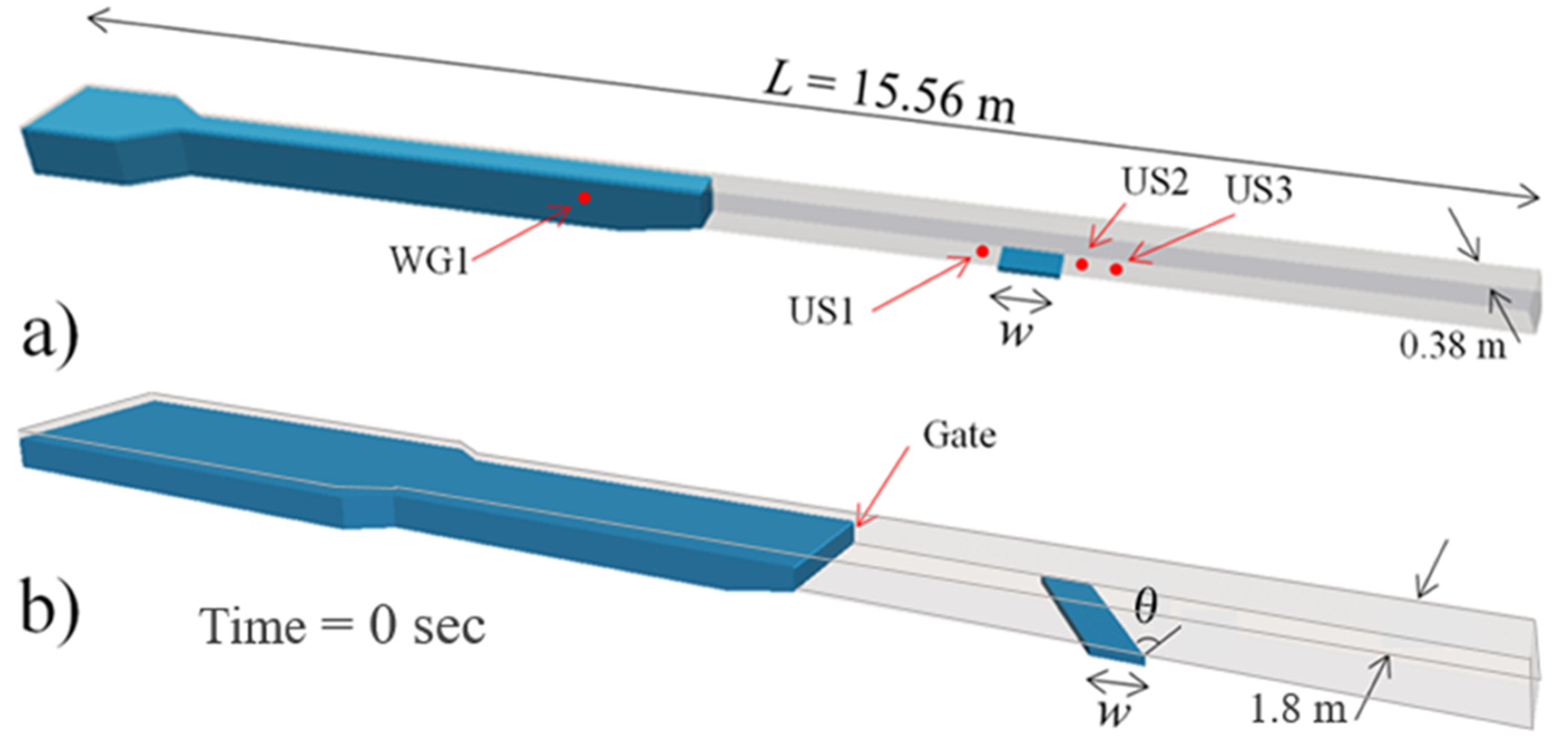
The flume boundary effect should be minimized in order to study the effect of canal orientation and the interaction of the bore front with the canal. The flume dimensions in the numerical domain were increased to 20.76 m × 1.8 m × 0.60 m in order to minimize the flume boundary effect (see
Figure 1).
The computational domain was extended laterally, by increasing its width, to eliminate the constriction effects of the sidewalls on the bore characteristics such as bore height, velocity, specific momentum, and specific energy [
2,
33,
38,
39]. Five tests with an impoundment depth of
do = 0.3 m and canal depth of
d = 0.10 m were modeled in order to study the effect of canal orientation, and sixteen tests were performed to investigate the effect of canal depth for an impoundment depth of
do = 0.40 m. In all cases, the canal width was constant, at
w = 0.60 m, and the orientation angles varied from 0° to 60° (see
Table 2).
Similar to the simulations performed for model validation, the initial values of the phase fraction, wave velocity, water height, pressure, and force were set to zero. For the initial boundary condition, the phase fraction of the reservoir was set to 1.0, indicating that the reservoir was filled with water.
Figure 1 shows the computational domains of the original and extended flumes and the water level at the initial condition (i.e.,
t = 0). The simulated flumes and water levels at the initial condition (i.e.,
t = 0) are shown using ParaView software, which is independent from OpenFOAM. In addition to the length of the tank, the flume was elongated from 1.2 m to 6.4 m in the flow direction to ensure that sufficient volume of impounded water was available for the simulation time of
t = 20 s.
All the boundaries of the numerical domain, except for the outlet, were set to the “wall-type boundary with no-slip condition” to ensure zero velocity at the wall and zero pressure at the water surface. The boundary condition for the flume outlet was set to the “zero gradient boundary condition”, which allowed water to exit the computational freely domain. Several flume geometries were generated to simulate flumes transversally perpendicular and various canal orientations with respect to the flume’s longitudinal axis. A mesh-independent analysis was performed to determine the optimum cell size in order to reduce computational cost while ensuring accuracy and mesh independency. The mesh-independent analysis was performed by systematically reducing the cell size from a coarse mesh to a refined mesh with a known aspect ratio [
42,
43].
A more refined mesh resolution was selected for downstream of the canal due to a significant change in the water surface and the need for accurate r at the locations of the monitoring equipment. The Ultrasonic wave Sensors (US) and the Acoustic Doppler Velocimetry (ADV) probes were located upstream and downstream of the canal. The US1 and ADV1 probes were located 0.2 m upstream of the canal, US2 and ADV2 were located 0.2 m downstream of the canal, and US3 and ADV3 were placed 0.58 m downstream of the canal.
Initially, the effect of mesh variation was examined using various mesh resolutions. The grid cell size was first refined for the entire computational domain of the flume and then locally around locations of specific interest, such as the locations of the ultrasonic sensors and the acoustic Doppler velocimetry probes. In the numerical simulations, the grid cell size was gradually decreased from the upstream end towards the downstream end of the flume, focusing on the location of the equipment. For flumes with lower-degree canal orientations (i.e., θ = 0°, 15°, and 30°), the cell size dimensions in the x-direction were set at 20 mm downstream of the gate, 30 mm upstream of the gate, and 40 mm upstream of the reservoir contraction. In the y- and z-directions, the cell size dimensions were set at 20 mm. For the flumes with higher-degree canal orientations (i.e., θ = 45° and 60°), the cell size dimensions in the x-direction were adjusted to 10 mm and 20 mm downstream and upstream of the gate, respectively. In the y- and z-directions, the cell sizes were adjusted to 10 mm. In the first part of this companion paper, three different turbulence models were employed in numerical simulation in order to establish the best agreement concerning the physical experiments. The time histories of the water surface levels and velocities at four locations were extracted from the numerical models, and the outcomes were compared with the measurements. The model validation was performed both in the absence and presence of a rectangular canal.
Another parametric study was undertaken in order to assess the performance and select the best turbulence model for the current simulation. To improve the accuracy of the simulations, three k-ε-based turbulent models (i.e., classic k-ε, Realizable k-ε, and RNG k-ε) were implemented. There was no significant difference between these three models; however, the root mean square error (RSME) displayed a slightly better agreement for the standard k-ε model. As a result, although the use of all three turbulence models provided good agreement with the experimental results, the standard k-ε model provided the best fit.
As such, the well-known standard k-ε turbulence closure model was further used for all the subsequent numerical simulations, as it provided the highest accuracy during the model validation (see Part One of the present companion paper). A dynamic time step was selected in the numerical simulations in order to ensure simulation stability and guarantee that the maximum Courant number was always less than unity. The computation times ranged from approximately four hours for the flumes with higher-degree canal orientations and coarse mesh, to 16 h for the flumes with lower-degree canal orientations and fine mesh.
3. Simulation Results
3.1. Momentum Flux Time Histories
The specific momentum flux per unit mass and per unit width of the flume was calculated as
hu2, where
h is the flow depth and
u is the flow velocity at a specific location. The three-dimensional numerical simulation results such as
h, and
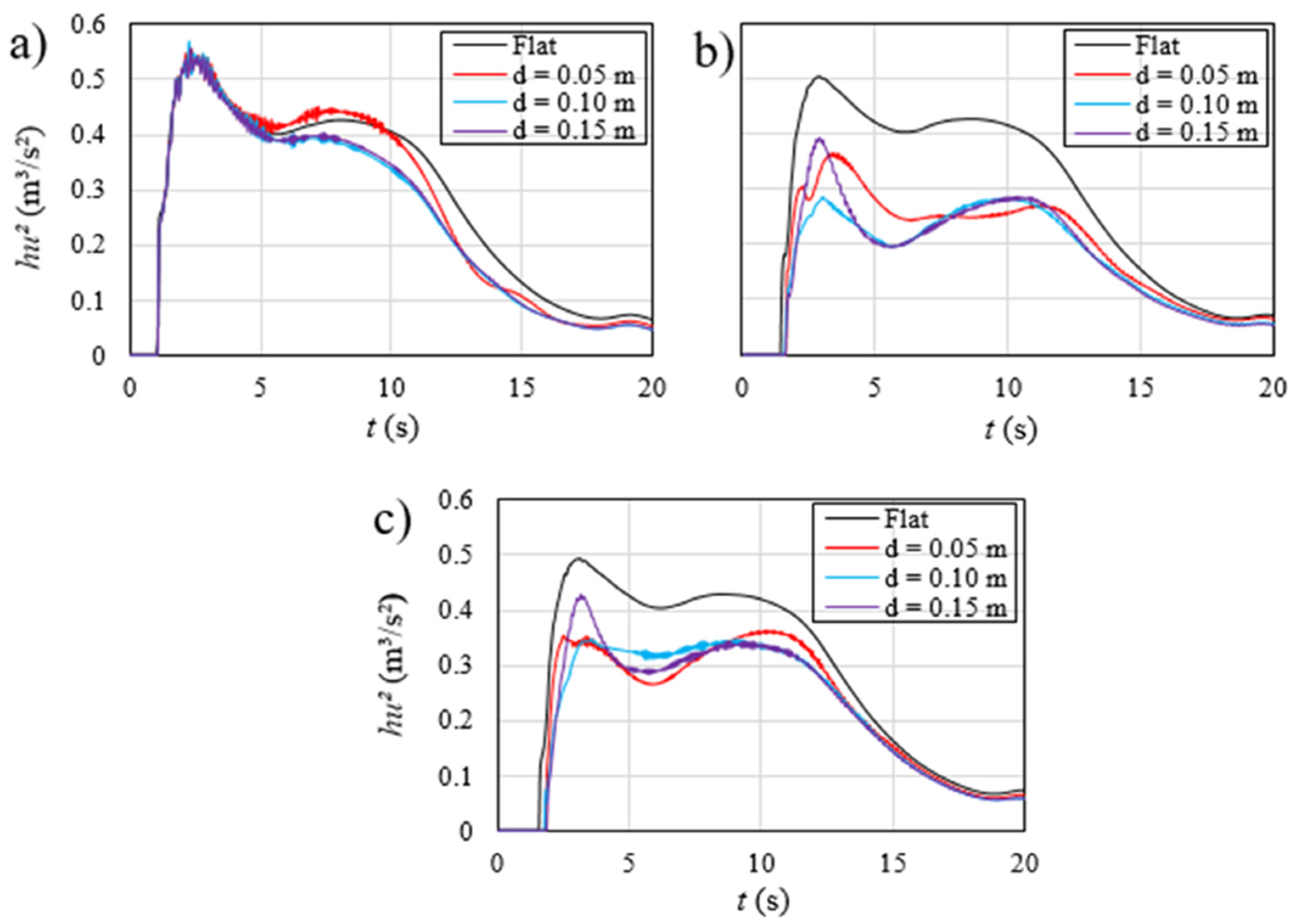
u can be obtained and extracted using object-oriented post-processing software (ParaView). The specific momentum simply contains the flow depth and velocity term, since adjacent positions have about the same pressure. The time histories of the specific momentum for different canal geometries and locations upstream and downstream of the canal were extracted from the numerical results, and are shown in
Figure 2. The latter shows the effects of mitigation canals on the time history of the specific momentum upstream and downstream of the canal. The impoundment depth for the tsunami-like wave is
do = 0.3 m. In this case, the width of the canal was kept constant (
w = 0.6 m) and different canal depths of
d = 0 m, 0.05 m, 0.1 m, and 0.15 m are compared. A large discrepancy was observed in the time histories of specific momentum in the presence of the canal and its absence. The difference between the maximum specific momentum compared to the absence of the canal showed an approximately 9.3% reduction between US2 and US3. For a canal depth of
d = 0.05 m (see
Figure 2b), the maximum specific momentum decreased by 27% and 13.7% at US2 and US3, respectively. However, for canal depths of
d = 0.10 m and 0.15 m, the maximum specific momentum decreased by approximately 28.3% and 27.9%, respectively, at US2, and by approximately 14.5% and 16.9% at US3, respectively. The instant at which the specific momentum reached its maximum magnitude were different upstream and downstream of the canal. This may be attributed to the canal-related turbulent flow that was generated.
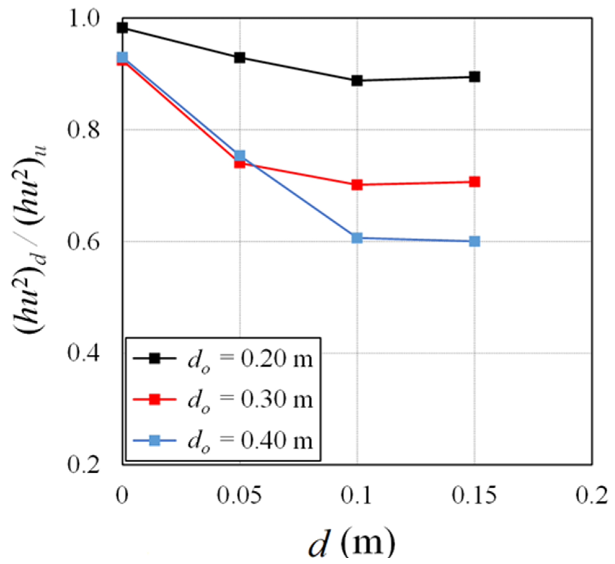
Figure 3 shows the time history of the ratio between the downstream and upstream peak specific momentums (
hu2)
d/(
hu2)
u with canal depth and for impoundment depths of
do = 0.2 m, 0.3 m, and 0.4 m.
The pressure of the specific momentum per unit mass per unit width is assumed to be approximately the same at the location 0.20 m upstream and the location at 0.2 m downstream of the canal. The lowest specific momentum ratio between the downstream and upstream peak of the canal was 60% for the canal depth of d ≥ 0.10 m and impoundment depth of do = 0.4 m, while the lowest specific momentum ratios between the downstream and upstream peak of the canal were 89% and 70% for the canal depth of d ≥ 0.10 m and impoundment depths of do = 0.2 m and 0.3 m, respectively. In contrast, the respective maximum specific momentum ratios for the impoundment depths of do = 0.2 m, 0.3 m, and 0.4 m were as high as 99%, 94%, and 93% of the specific momentum ratio without a canal. It was noted that for the 0.40 m impoundment depth, the maximum specific momentum ratio decreased to approximately 60% as the canal depth was increased from d = 0 m to d = 0.10 m. Lower reductions were observed for the impoundment depths of do = 0.2 m and 0.3 m. Generally, the variation of the ratio of downstream to upstream peak specific momentum decreased as the impoundment depth increased.
3.2. Time History of Mean Flow Energy
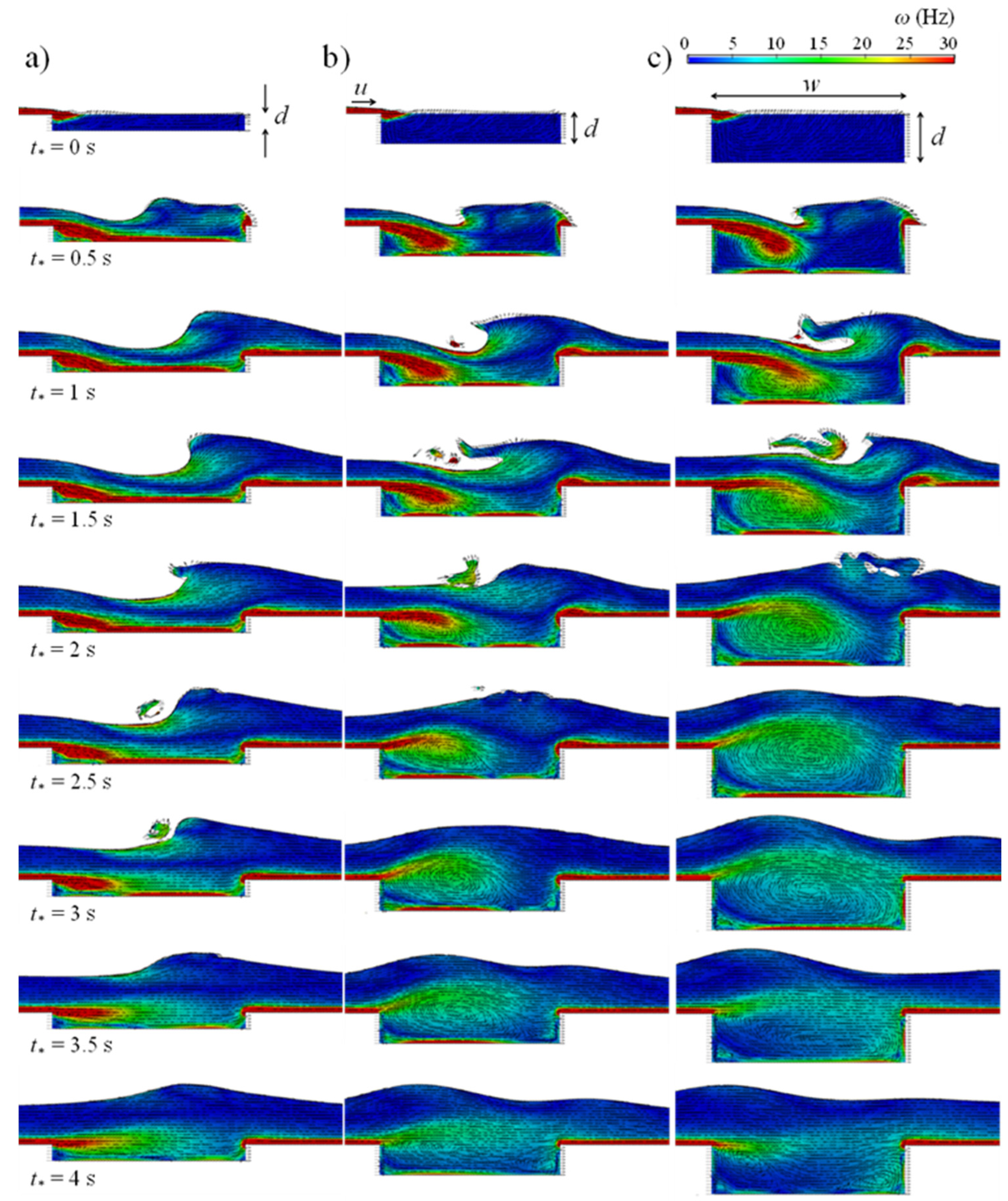
Figure 4 shows the effects of canal depth on time histories of the contour plots of mean flow energy for a bore passing over a canal from an impoundment with a depth of
do = 0.3. The canal width in all tests was kept constant (
w = 0.6 m), and different canal depths of
d = 0.05 m, 0.10 m, and 0.15 m were tested.
Figure 4a shows the contour plot of the shallowest canal (
d = 0.05 m). The time at which the bore front reached the mitigation canal was set as the initial time of
t∗ = 0. At
t∗ = 0.50 s, the bore front plunged into the canal without reaching its bottom yet, and the jet stream of the maximum mean flow energy reached half of the canal width in longitudinal direction. The jet stream then slowly moved in the downstream direction. At
t∗ = 1.0 s, the jet stream of the maximum mean flow energy touched the bottom of the canal and reached a maximum distance of 0.47 m from the upstream edge of the canal. At
t∗ = 1.5 s, the jet stream of the maximum mean flow energy reached its farthest distance from the upstream canal edge at nearly 0.50 m, which was more than 80% of the canal width. At
t∗ = 2 s, the jet stream of the maximum mean flow energy moved back in the upstream direction, and gradually rose with time from the bottom of the canal until it reached the horizontal bed of the flume at
t∗ = 3 s. The time histories in the contour plots of the mean flow energy with time in the medium (
d = 0.10 m) and deep (
d = 0.15 m) canals indicated that the jet streams of the maximum mean flow energy reached their maximum length at
t∗ = 1.5 s and at approximately 0.41 m and 0.47 m, respectively, (see
Figure 4b,c).
The mean flow energy,
K, for different canal geometries, different locations upstream and downstream of the canal, and the same impoundment depth were calculated using
K = (
u2 +
v2 +
w2)/3, where
u, v, w were the components of the flow velocity in the
x-,
y-, and
z-directions, respectively.
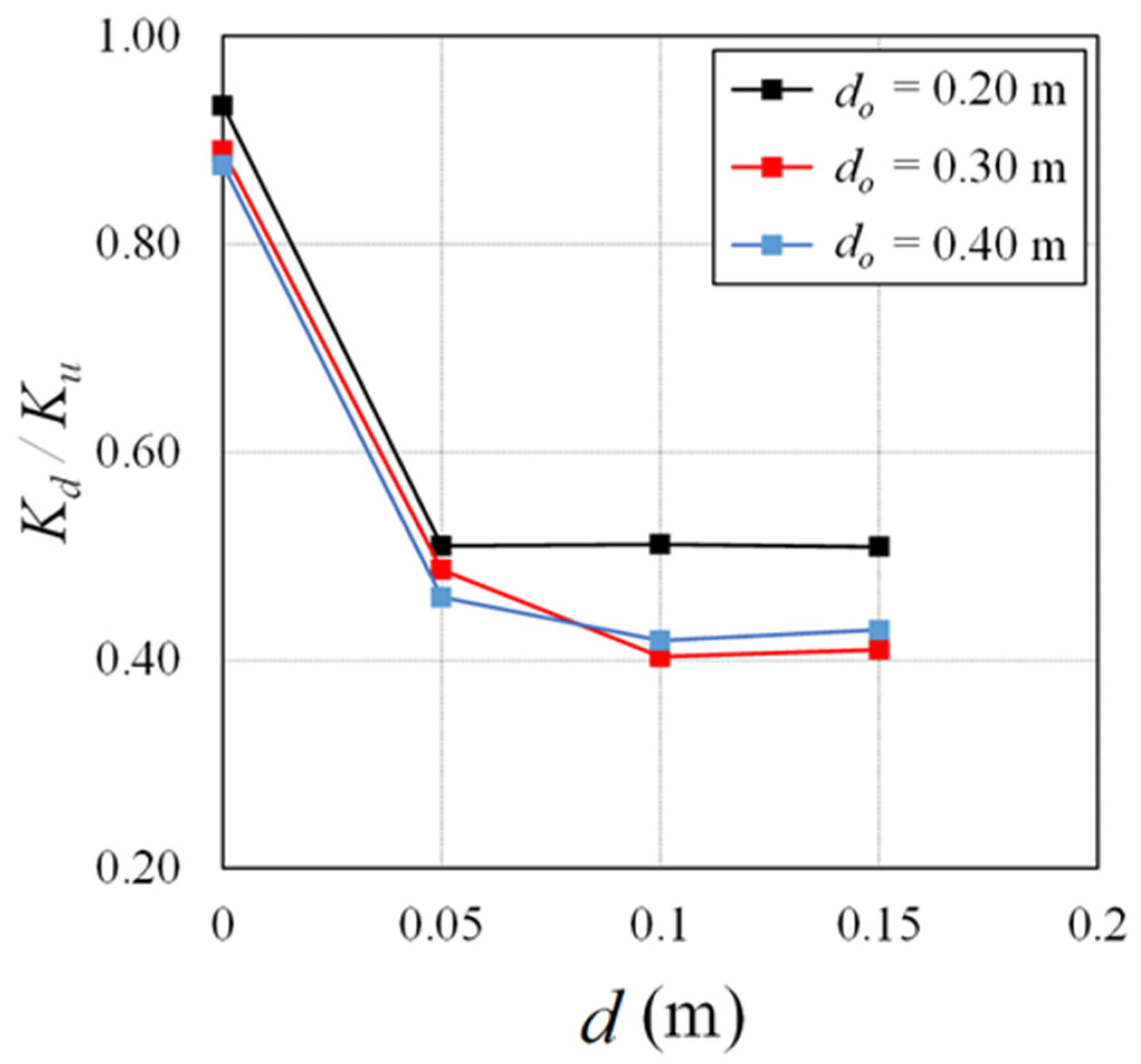
Figure 5 shows the variations in the ratio of mean flow energy before and after the canal,
Kd/Ku, with canal depths and for different impoundment depths of
do = 0.2 m, 0.3 m, and 0.4 m.
The lowest mean energy ratio, with the value of Kd/Ku = 41%, was observed in the test with the canal depth of d = 0.10 m and impoundment depth of do = 0.3 m. In contrast, the maximum mean energy ratios were observed in tests without a canal with the values of 93%, 89%, and 87% for do = 0.2 m, 0.3 m, and 0.4 m, respectively. The variations in the ratio of mean energy noticeably declined as the canal depth increased from d = 0 m to d = 0.05 m. The energy ratios were almost constant as the canal depth increased from d = 0.10 m to d = 0.15 m, and they were independent of impoundment depth. For both canal depths of d = 0.10 m and 0.15 m, there were nearly the same minimum specific momentum and mean energy ratios and that they were independent of impoundment depth.
The total specific energy per unit width,
E, was calculated based on the water depth and velocity at different measurement locations, as
E =
h +
u2/(2
g). It only contains the water depth and velocity term, since nearby locations have approximately the same pressure.
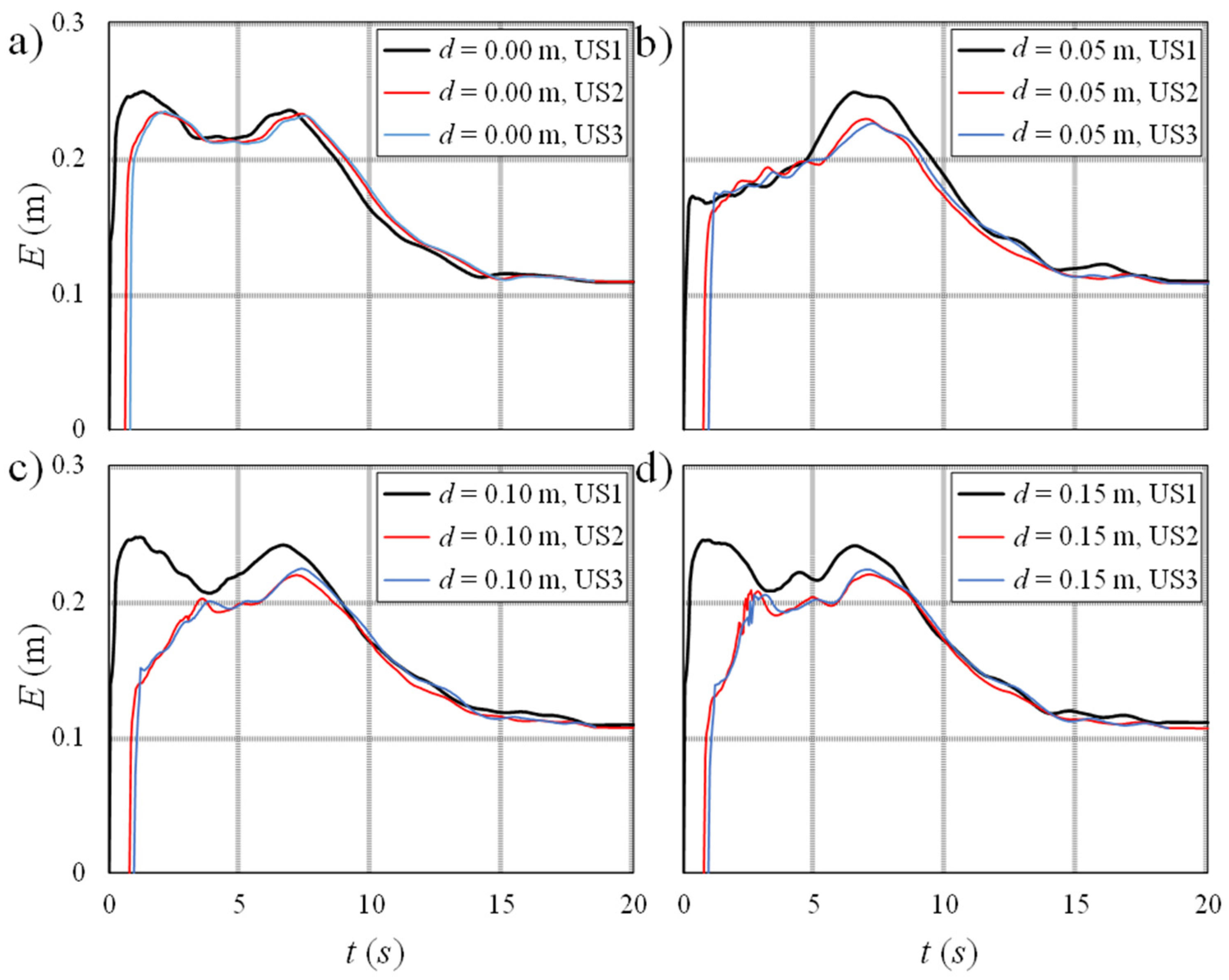
Figure 6 shows the effects of a mitigation canal on the time histories of specific energy,
E, of a bore before and after the canal. The impoundment depth of the bore was
do = 0.3 m, the canal width was constant with a value of
w = 0.6 m, and the canal depths were
d = 0 m, 0.05 m, 0.1 m, and 0.15 m.
Figure 6a shows the time histories of the specific energy over the horizontal bed. The peak specific energy decreased by approximately 5.7% between the measurement locations of US2 and US3 (see
Figure 6a). For the tests with a canal depth of 0.05 m (see
Figure 6b), the peak total specific energy decreased by approximately 7% and 7.6% of that measured at the points of US2 and US3, respectively. The difference between the peak total specific energies at the two measurement locations increased in tests with canal depths of
d = 0.1 m and 0.15 m. As can be seen in
Figure 6c,d, the peak specific energies decreased by approximately 10.2% and 9.6% for canal depths of
d = 0.10 m and 0.15 m, respectively.
3.3. Vertex Structure
Figure 7 shows the time histories in the contour plots of bore vorticity,
ω, and the velocity vector fields for a constant canal depth of
w = 0.6 m, impoundment depth of
do = 0.3 m, and different canal depths of
d = 0.05 m, 0.1 m, and 0.15 m.
A river bore is an upstream proceeding transition between two various flow depths generally produced by tidal pressure. Analogous flows can be created in structured environments such as wave flumes, and many experimental investigations have been achieved to discover some of the key characteristics of bores. Thus, the relatively slight inconsistency with the experiments could be attributed partially to the vorticity induced by the discharge used to create the undular bore. Vorticity, in particular, appears to be a significant factor in the bores produced by a constant discharge. Some authors [
44,
45] have indicated the significance of bottom friction on the appearance of an undular bore. In a river bore, if the circumstances are appropriate, an approximately steady profile of undulations can be observed. A bore can be categorized by the bore strength or Froude number [
46,
47,
48,
49,
50,
51,
52,
53].
Figure 7a shows the time histories in the vorticity contour plots for a canal depth of
d = 0.05 m, and the area of maximum vorticity is marked as
ω ≥ 30 Hz. As shown in
Figure 7a, at
t∗ = 0.5 s, the peak vorticity formed in the vicinity of the upstream edge of the canal and extended 0.17 m downstream of the upstream wall of the canal. A vortex eye formed in the vicinity of the upstream edge of the canal. At
t∗ = 0.5 s, the vortex eye formed at approximately 0.05 m downstream of the upstream wall of the canal, and it advanced slowly as the bore advanced through the canal. At
t∗ = 3.5 s, the maximum vorticity reached its farthest distance from the upstream wall at approximately 0.20 m from the upstream wall, and then decreased at
t∗ = 4.0 s. At
t∗ = 4.0 s, the vortex eye reached its farthest distance from the upstream wall of the canal at nearly 0.12 m. In the numerical simulation, the bore front plunged into the canal, generating a surface hydraulic jump. The bore height then increased due to an increase in pressure force caused by the surface hydraulic jump at the downstream edge of the canal. The bore front then transferred more momentum to the volume of water in the canal, resulting in a strong surface jump reaching the downstream edge of the canal. The bore energy decreased as it passed through the canal. The upward deflection due to pressure force caused by the surface hydraulic jump of the greatest bore vorticity expanded the recirculation zone upstream of the canal and gradually pushed the vortex eye downstream.
As shown in
Figure 7b,c, the locations of maximum vorticity in the medium depth and the deep canals reached the upstream wall at 0.24 m for 0.5 s ≤
t∗ ≤ 2.0 s and 0.30 m at
t∗ = 1.0 s, respectively. Then, the maximum bore vorticity decreased with time. The vortex eyes in the medium and deep canals gradually advanced towards the downstream wall of the canal until they reached their longest distance from the upstream wall of the canal at 0.26 m (
t∗ = 3.5 s) and 0.30 m (
t∗ = 3 s), respectively. The location of the maximum bore vorticity in the water vorticity contour plots increased as the canal depth increased, indicating more transition of momentum and energy as the canal depth increased. This happened due to the higher capability of the deep canal to absorb the bore and dissipate the energy generated by the bore-canal interaction.
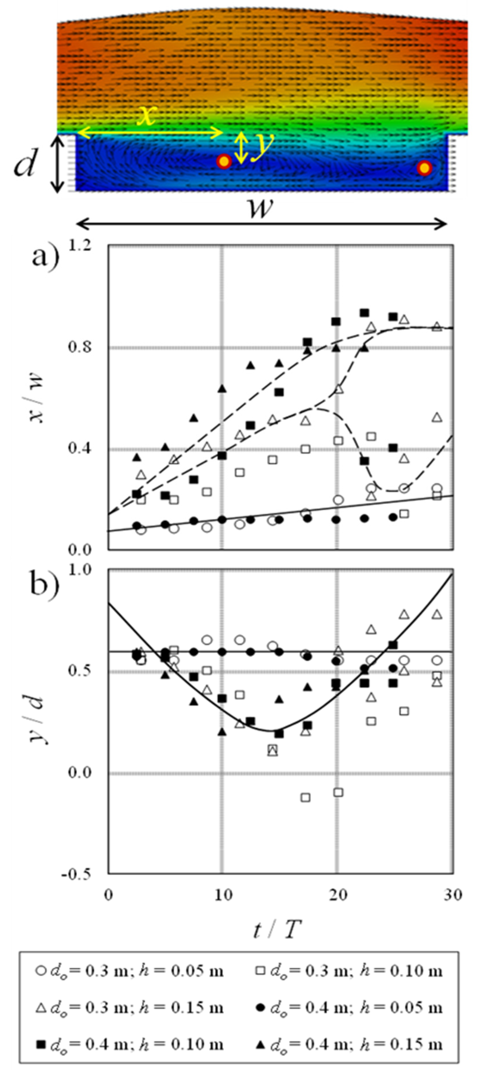
Figure 8 shows the variations in the location of the eye of the vortex inside the canal as a function of the non-dimensional time
t/T for bores generated from impoundments depths of
do = 0.30 m and 0.40 m.
The horizontal,
x, and the vertical,
y, distances of the eye of the vortex from the walls of the canal were normalized with the canal width and depth as
x/
w and
y/
d, respectively.
Figure 8a shows the correlations between the normalized time,
t/
T, and normalized horizontal distance of the vortex eye,
x/
w, for bores with different canal and impoundment depths. As shown in this figure, the normalized horizontal distance of the vortex eye increased linearly with time for the canal depth
d = 0.05 m. The maximum variations of
x/
w for the canal depth
d = 0.05 m were 0.26 and 0.14 for
do = 0.30 m and 0.40 m at
t/
T = 29 and 25, respectively. However, for the canal depths,
d = 0.10 m and 0.15 m, the variations of
x/w gradually increased until reached peak values of 0.45 and 0.80 for
do = 0.30 m and 0.40 m, respectively. For the canal depths
d = 0.10 m and 0.15 m, the variations of
x/
w with time indicate a gradual increase until the separation of the vortex eye began at
x/
w = 0.58 and
t/
T = 18. Following the separation, the variations of
x/w with time slightly increased to reach the
x/
w of the deep canal with the highest impoundment depth.
Figure 8b shows the variations of
y/
d with
t/
T for different impoundment and canal depths. The vertical distance from the canal bed was found to be time independent in shallow canals (i.e.,
d = 0.05 m), and the value of
y/
d was found to be equal to 0.59. However, for the canal depth
d = 0.10 m, the variations in
y/
d started from
y/
d = 0.59 and gradually decreased until reaching the lowest value of
y/d = 0.20 at
t/
T = 15. As time passed, the value of
y/
d increased from the minimum to approximately the same range as
y/
d = 0.59. In the deep canal (
d = 0.15 m), the variations of
y/
d with time were similar to those with the medium depth canal and reached their minimum value at
y/
d = 0.20.
3.4. Time Histories of Turbulent Kinetic Energy
The effects of canal depth on the time histories of the turbulent kinetic energy,
k, are shown in
Figure 9.
The impoundment depth and canal width were kept constant, with values of do = 0.3 m and w = 0.6 m, respectively. In this figure, the contour plots of the turbulent kinetic energy for different canal depths of d = 0.05 m, 0.10 m, and 0.15 m are presented. At t∗ = 0.5 s, the turbulent kinetic energy of the bore jet stream developed in the vicinity of the upstream wall of the canal and propagated gradually downstream as the bore passed over the canal. At t∗ = 1.5 s, the area with the maximum turbulent kinetic energy reached its highest value in the shallow, medium, and deep canals. The region of the bore’s maximum turbulent kinetic energy (i.e., k = 0.20 m2/s2) started disappearing gradually once the bore reflecting in the upstream direction of the canal. Then, at t∗ = 2.0 s, the area of peak turbulent kinetic energy started decreasing in time. However, at t∗ = 3.5 s, the region with the maximum turbulent kinetic energy remained in the shallow- and medium-depth canals, but completely disappeared in the deep canal. It can be concluded that the region of maximum turbulent kinetic energy disappeared rapidly as the canal depth increased.
Figure 10 shows the effects of canal depth on the time histories of the energy dissipation rate,
ε, for tests with an impoundment depth of
do = 0.3 m and canal width of
w = 0.6 m, respectively.
A region with an energy dissipation rate of 2 m2/s3 is labeled as an area with a strong energy dissipation rate. A region with a strong energy dissipation rate formed in the middle of the canal and decreased with time. The region of strong dissipation gradually moved towards the downstream part of the canal. For shallow, medium, and deep canals, the strong energy dissipation region reached the longest distance from the upstream wall of the canal at t∗ = 1.5 s with values of 0.55 m, 0.47 m, and 0.54 m, respectively. Those regions gradually moved back towards the upstream wall of the canal. The upward deflection of the region of maximum energy dissipation increased the water recirculation over the canal and gradually moved towards the upstream wall of the canal. In the medium and deep canals, the region of maximum energy dissipation disappeared at t∗ = 3 s and 2.5 s, respectively, while this region still appeared in the shallow canal even at t∗ = 3.5 s. The contour plots of the energy dissipation rate indicated that the overall energy dissipation rate decreased with increased canal depth.
5. Discussion
The mitigation of dam-break waves propagating over a rectangular canal located perpendicular on the direction of the flow and which is fully filled with water was analyzed numerically. The effects of the canal depth and its orientation were investigated by modeling this canal with a constant width of w = 0.6 m, depths of d = 0.0 m, 0.05 m, 0.10 m, and 0.15 m, and with orientations of θ = 0°, 15°, 30°, 45°, and 60°. The peak specific momentum without the presence of the canal exhibited a decrease of approximately 9.3% at the locations of US2 and US3 compared to US1. For the 0.05 m canal depth, the peak specific momentum decreased by 27% and 13.7% at US2 and US3, respectively. For canal depths of 0.10 m and 0.15 m, however, the peak specific momentum declined by almost 28.3% and 27.9% at US2, respectively, and declined by nearly 14.5% and 16.9%, respectively, at US3. Similarly, the differences in the maximum specific energy over a horizontal bed exhibited a nearly 5.7% decrease at the locations of US2 and US3. For the 0.05 m canal depth, the maximum specific energy decreased by approximately 7.0% and 7.6% at US2 and US3, respectively, although the 0.10 m and 0.15 m canal depths exhibited higher differences compared to the 0.05 m canal depth and horizontal bed, such as the maximum specific energies decreasing by around 10.2% and 9.6%, respectively, at both locations downstream of the canal. Overall, higher downstream variations were found in the time histories of specific momentum and energy in the presence of a canal.
The non-dimensional specific momentum and mean flow energy downstream and upstream of the canal exhibited similar patterns for the three impoundment depths and three canal depths. For the 0.4 m impoundment depth, the lowest non-dimensional specific momentum was as low as 60% of that of the 0.10 m and 0.15 m canal depths, while the lowest non-dimensional specific momentums were 70% and 89% for the 0.3 m and 0.2 m impoundment depths, respectively, and canal depths ≥ 0.10 m. Additionally, the lowest non-dimensional mean flow energy was as low as 41% of that of the 0.10 m canal depth and the 0.3 m impoundment depth. For the three impoundment depths, the 0.10 m and 0.15 m canal depths had the lowest, and nearly equal, non-dimensional specific momentum and mean flow energy.
It can be inferred that the jet stream of maximum vorticity in the shallow, medium-depth, and deep canals reached their longest distances at 0.20 m, 0.24 m, and 0.30 m, respectively, from the upstream edge of the canal. The longest movement of the vortex eyes in the shallow, medium-depth, and deep canals were 0.12 m, 0.26 m, and 0.30 m, respectively, from the upstream edge of the canal. Additionally, the normalized horizontal distance of the eye of the vortex x/w gradually increased with time, reaching maximum values of 0.26 and 0.14 for do = 0.30 m and 0.40 m, respectively, for d = 0.05 m. The variations in x/w with time increased steadily for the canal depths of d = 0.10 m and 0.15 m and reached their maximum values of 0.45 and 0.80 for do = 0.30 m and 0.40 m, respectively. For the medium-depth and deep canals, the variations in x/w showed a steady rise until separation of the eye of the vortex occurred at x/w = 0.58 and t/T = 18. The normalized vertical distance of the vortex eye y/d was found to be time-independent for d = 0.05 m, with a value of 0.59. However, the variations y/d gently declined for d = 0.10 m from y/d = 0.59 until reaching the lowest value of y/d = 0.20 at t/T = 15. Then, the value of y/d rose from its lowest point to about y/d = 0.59. Similarly, the variations in y/d with time reached their minimum value at y/d = 0.20 for d = 0.15 m.
The region of maximum turbulent kinetic energy reduced gradually as after the initial bore passed over the canal, indicating a dissipation of energy due to the existence of the mitigation canal, and it may be concluded that the region of maximum turbulent kinetic energy vanished with increased canal depth. Additionally, the maximum penetration length of the energy dissipation formed in the middle of the canal and then traveled steadily downstream. The maximum energy dissipation regions reached their longest distances from the upstream edges of the shallow, medium, and deep canals with values of 0.55 m, 0.47 m, and 0.54 m, respectively. Then, the maximum bore jet stream moved slowly back in the upstream direction of the canal.
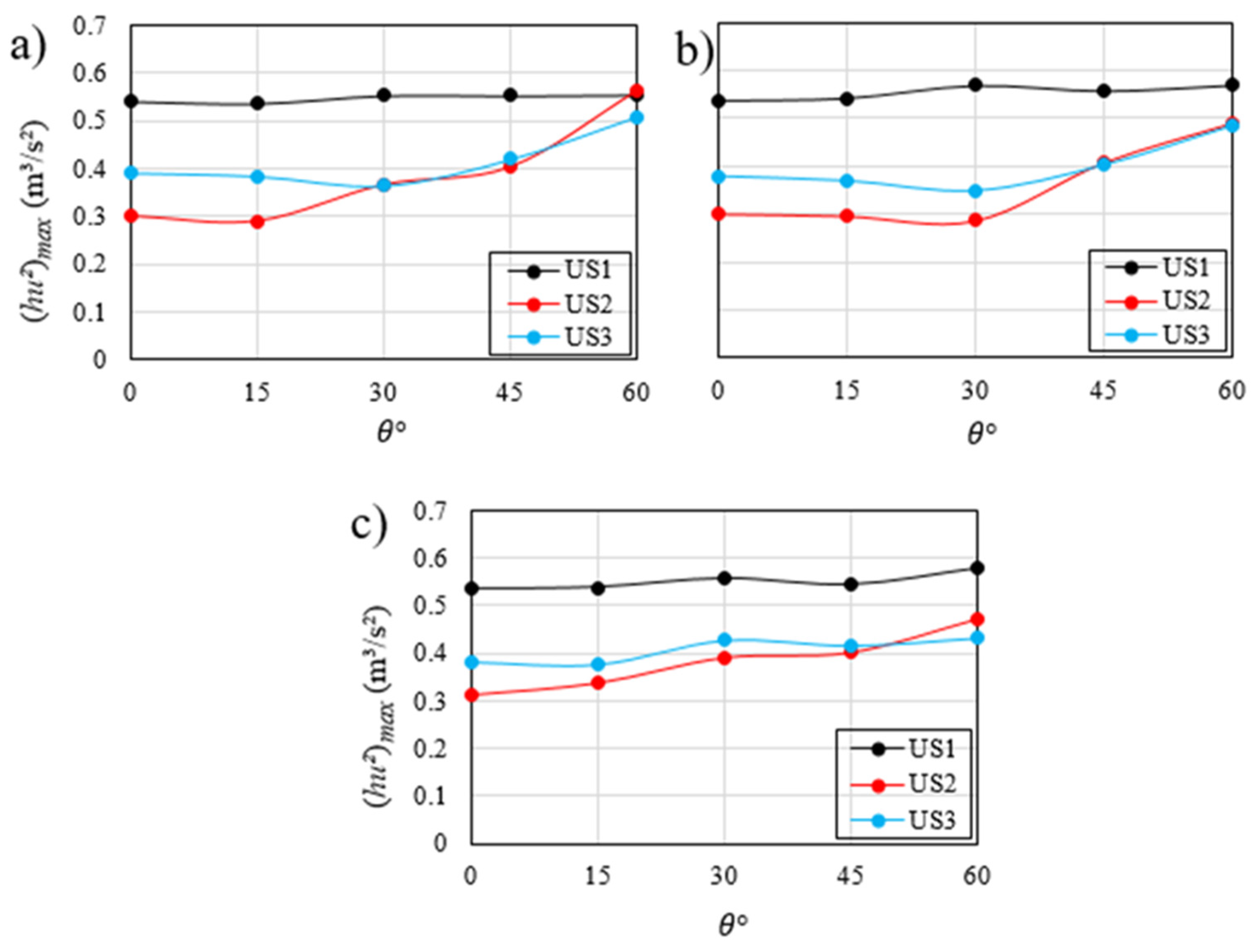
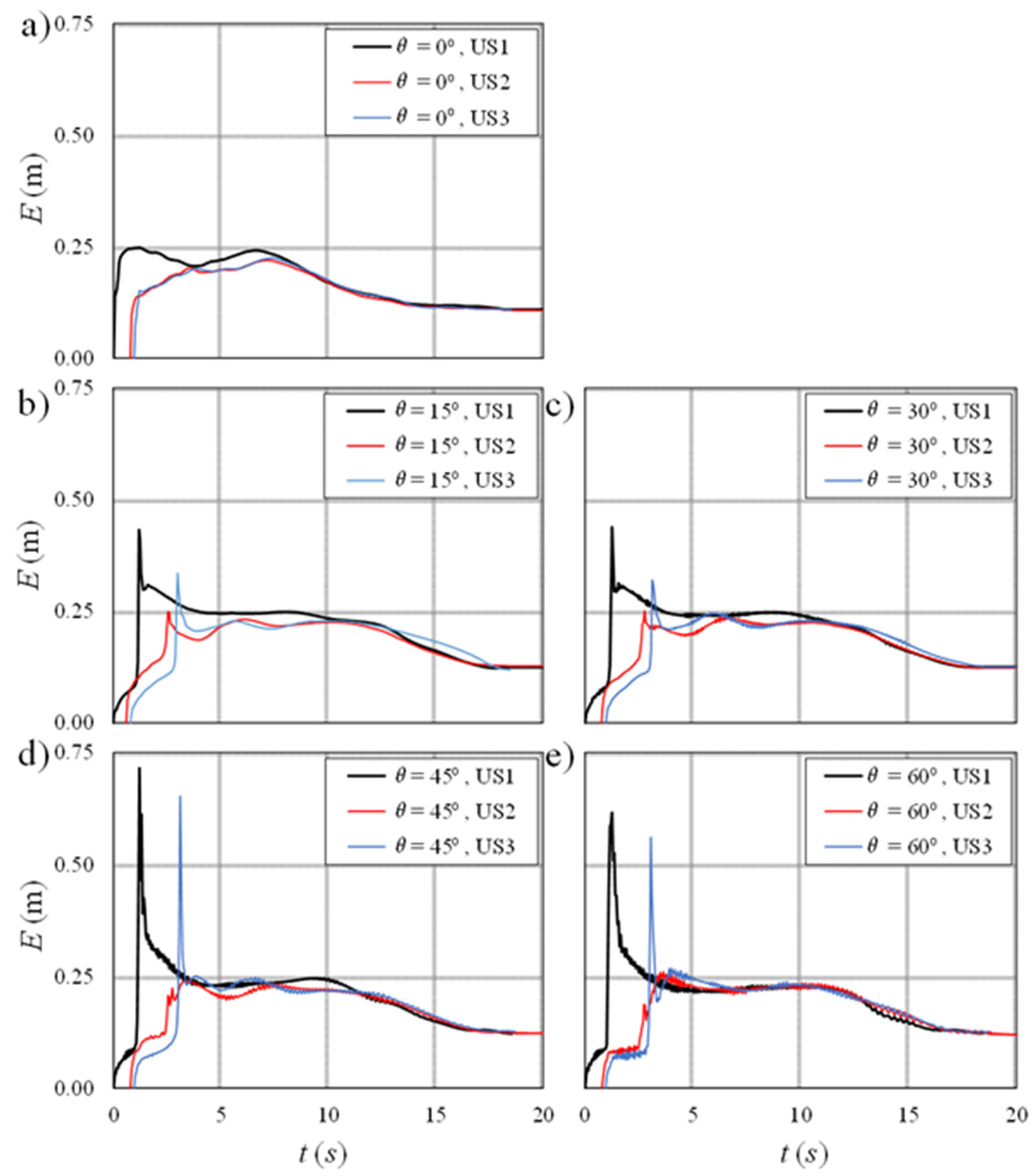
It can be observed that with the canal orientation of θ = 45°, the maximum specific momentum reached its highest value at the location of US3. The maximum specific momentum of θ = 45° at US3 was approximately 5 times greater than the maximum specific momentum for θ = 0° at the corresponding location. However, the maximum specific energy approached its highest value of θ = 45° at US1. In the case of θ = 45°, the maximum specific energy was nearly 3 times higher than that of θ = 0° at US1, although the values of the maximum specific momentum and maximum specific energy remained almost equal at US2 for the different canal orientations.
The correlation of maximum specific momentum with canal orientation for d = 0.05 m shows that the lowest (best) maximum specific momentums at the US2 and US3 sensors for θ = 15° and 30° were 0.29 m3/s2 and 0.36 m3/s2, respectively. For the canal depth of d = 0.10 m, the lowest (best) maximum specific momentums at the positions of US2 and US3 and for θ = 30° were 0.29 m3/s2 and 0.35 m3/s2, respectively, while the lowest (best) peak specific momentums for θ = 0° and 15° were 0.31 m3/s2 and 0.38 m3/s2, respectively, for the canal depth of d = 0.15 m. In the first part of this companion paper, three different numerical turbulence models, i.e., the classic k-ε, Realizable k-ε, and RNG k-ε models, were used in order to determine the best match with the physical experiments. The experimental and numerical water surface profiles matched well, with a root mean square error (RMSE) of less than 6.7% and a relative error of less than 8.4%. Although all of the numerical simulations agreed well with the experimental results, the standard k-ε model provided the best match. As a result, the standard k-ε turbulence model was employed to investigate the present work.
The strong turbulent formation of bores within and around canals increase specific momentum and energy losses downstream. Higher peak specific momentum fluxes were observed at US1, with nearly 33.9%, 49.6%, and 29.8% for bores proceeding over canals with depths of d = 0.05 m, 0.10 m, and 0.15 m, respectively, in comparison with corresponding measurements at US2. Additionally, when compared to measurements taken at US3, US1 had greater bore specific momentum flux peaks, of nearly 34.1%, 38.6%, and 23.1%, for bores propagating over canals with depths of d = 0.05 m, 0.10 m, and 0.15 m, respectively.


