
On the Propagation of Hydrothermal Waves in a Fluid Layer with Two-Way Coupled Dispersed Solid Particles


Department of Mechanical and Aerospace Engineering, University of Strathclyde, James Weir Building, 75 Montrose Street, Glasgow G1 1XJ, UK
Fluids 2022, 7(7), 215; https://0-doi-org.brum.beds.ac.uk/10.3390/fluids7070215
Submission received: 4 June 2022
/
Revised: 17 June 2022
/
Accepted: 21 June 2022
/
Published: 23 June 2022
Abstract
:The propagation of hydrothermal waves in a differentially heated shallow open cavity filled with a complex fluid (a mixture of an oil with solid spherical metallic particles) is investigated in the framework of a hybrid numerical two-way coupled Eulerian–Lagrangian methodology. We explore the response of this system to the solid mass fraction (mass load) and the particle size (Stokes number). The results show that particles and related (inertial and drag) effects can cause appreciable modifications in the properties of the wave, leading to a shrinkage of its velocity of propagation. Interesting dynamics can also be seen in terms of particle patterning behavior as the Stokes number is increased. Due to the joint action that distinct traveling rolls exert on the dispersed solid mass, related accumulation loops induced by centrifugal effects are progressively distorted and finally broken. Particles simply tend to cluster (as time increases) along the lower periphery of the main Marangoni circulation and, as a result of this mechanism and the different velocities of the return flow and the hydrothermal disturbance, a wavy boundary is formed, which separates the upper particle-rich area from a relatively depleted region next to the bottom wall.
1. Introduction
Hydrothermal waves (HTWs) represent the preferred mode of supercritical Marangoni convection in a variety of geometrical configurations and for different fluids (including liquid metals, molten salts or oxides and a plethora of transparent and/or organic liquids). The first experimental observation of these phenomena dates back to the work by Schwabe and Scharmann [1], who revealed their existence in liquid bridges. Later, Smith and Davis [2] determined the properties of these waves (the critical value of the Marangoni number, the direction of propagation of the disturbance with respect to the basic flow and the related wavenumber and wavelength as a function of the Prandtl number, Pr) applying the typical protocols of the linear stability analysis (LSA) to a layer of infinite extent with adiabatic top and bottom boundaries.
Yet in the framework of LSA, Priede and Gerbeth [3] considered the alternate case with a conducting boundary on the bottom (assumed to mimic the effect of an external metallic container, with the free liquid/gas surface retaining an adiabatic behavior). Subsequent studies were essentially devoted to a characterization of these phenomena for different boundary conditions (of a thermal and/or geometrical nature). As an example, several experiments (Daviaud and Vince [4] for Pr = 10.3; Gillon and Homsy [5] for Pr = 9.5; De Saedeleer et al. [6] for Pr = 15; Garcimartìn et al. [7] for Pr = 10, 15 and 30; Pelacho and Burguete [8] and Pelacho et al. [9] for Pr = 10.3; Burguete et al. [10]) indicated that the properties of the emerging flow may depend significantly on geometrical factors. Along these lines, it is certainly worth citing Pelacho et al. [11], as these authors conducted a series of tests expressly conceived to characterize the emergence of waves in containers whose dimensions (height, width and length) could be continuously changed. Peltier and Biringen [12], Xu and Zebib [13] and Tang and Wu [14] numerically explored these behaviors for rectangular containers of finite size with various aspect ratios. Studies addressing the presence of a topography on the bottom of the considered physical domain in the form of a backward-facing or forward-facing step (or a combination of both geometrical features resulting in a central obstruction) are relatively recent (Lappa [15]). Steady gravity or oscillatory accelerations (resulting from the application of vibrations to the container hosting the liquid) are also known to have a significant impact on the dynamics of the hydrothermal waves, leading in some cases to their suppression (Parmentier et al. [16]) or to the emergence of new waveforms (standing waves or waves traveling in other directions, Lappa [17]).
Additional degrees of freedom are represented by the possibility to alter the kinematic and thermal conditions at the free interface by blowing a current of air with a desired velocity and temperature in a direction parallel to the surface itself (Shevtsova et al. [18]) or to induce a solidification process in the liquid by lowering the temperature on the cold side under the threshold required for phase transition (from liquid to solid) to occur (Lappa [19], Salgado Sanchez et al. [20]). As an additional example witnessing the richness of the considered problem in terms of influential factors and system response, Ospennikov and Schwabe [21] revealed that the HTWs can be artificially suppressed (leading to stationary rolls) in experimental configurations where the return flow does not exist (these researchers suppressed the return flow using channels and side channels with lower flow resistance compared to that of the return flow).
Although the exploration of the sensitivity of these phenomena to intrinsic and environmental factors may appear as exhausted given the number of valuable efforts described above, most recently a completely new line of inquiry has been originated by the discovery that these waves can support the formation of ordered structures produced by particles (tracers initially dispersed in liquid bridges for visualization purposes). Such findings (Schwabe et al. [22]) have stimulated a number of research works focusing on aspects relating to the patterning behavior in these systems for conditions in which the presence of the dispersed phase is expected not to influence the properties of the carrier flow (dilute dispersions, see, e.g., Schwabe et al. [23], Schwabe and Mizev [24], Pushkin et al. [25], Melnikov et al. [26], Lappa [27,28,29,30], Kuhlmann et al. [31], Gotoda et al. [32,33], Lappa [34], Melnikov and Shevtsova [35], Capobianchi and Lappa [36,37,38], Sakata et al. [39]).
Given the lack of analyses specifically devoted to this topic, in the present work, we concentrate on the fundamental interaction of such traveling waves with dispersed particles for situations in which the back influence of particles on the background fluid flow cannot be neglected (this actually brings in a new degree of freedom not addressed by earlier studies). In particular, given the significant interest attracted by such a configuration in the past and its simplicity, we consider the case of a differentially heated laterally bounded layer, i.e., a rectangular open cavity in microgravity conditions (no buoyancy effects). Although properly capturing the spanwise component of the HTWs would require fully three-dimensional (3D) simulations, in line with similar attempts in the literature (see, e.g., [12,13,14,15,19]), we base the simulations on a two-dimensional (2D) one-layer model. Clearly, such a simplification is equivalent to considering an ‘idealized’ setting where any processes that depend on the details of the third (spanwise) dimension are excluded. Nevertheless, our endeavor originates from the two-fold intention to (1) look directly at the physical (fundamental) processes involved for high-Prandtl-number fluids, which are believed to be ‘captured’ with an acceptable degree of approximation by a 2D model, and (2) contain the otherwise not affordable simulation time which would be required by parametric 3D computations.
2. Mathematical and Numerical Model
The influence of a dispersed phase on HTWs is still a matter of debate. As outlined in the Introduction, existing theoretical and numerical studies have been limited essentially to dilute systems in which the effects of particles on the background flow could be ignored.
A full understanding of such a problem would require it to be tackled in a consistent way on several scales. Clearly, the first of these scales concerns the emergence of waves as a result of the primary instability of Marangoni flow. This means that some care is needed to ensure that the mathematical model and the related computational technique adequately capture such large-scale phenomena.
The next level of this hierarchy is that connected with the dispersed phase itself. Proper simulation of particle motion requires adequate understanding of the processes relating to the transfer of momentum and thermal energy from the surrounding fluid to particles and vice versa. This subject should therefore be regarded as a typical example of problems driven by the interplay of large-scale (HTW) and small-scale entities and processes (particles and their displacement in time), for which, in general, a multiscale (and multiphysics) approach is needed.
Given these premises, we follow here the same strategy recently implemented by Lappa [40], i.e., a combined Eulerian–Lagrangian approach where the equations accounting for the liquid and solid mass are properly coupled through the presence of ‘interphase exchange terms’. As further detailed in the next section, these coupling terms only relate to a subset of the involved transported quantities as in the present case the particles do not dissolve in the carrier fluid (i.e., they behave as an immiscible phase).
2.1. Fluid Governing Equations
For the liquid phase, we consider the classical continuum (Navier–Stokes) equations, which, for an incompressible Newtonian fluid, simply read
where the vector V accounts for the fluid velocity components [u, v] along the x and y directions, respectively, p is the pressure and T is the temperature; moreover, ρ, μ, λ and Cv are the fluid density, dynamic viscosity, thermal conductivity and specific heat at constant volume, respectively (all assumed to be constant).
These equations also include at the right-hand side the aforementioned interphase coupling terms, by which the diverse effects of particle dynamics of fluid flow can be properly accounted for. These are formally represented by the vector quantity Sm and the scalar SE at the right-hand side of Equations (2) and (3), respectively. As mentioned before, the continuity equation (Equation (1)) lacks such a term as particles are considered immiscible entities, and therefore the overall masses of the liquid and the solid phases are conserved separately.
2.2. Particle Tracking Equations
As shown in Section 2.1, proper implementation of a two-way coupling strategy requires ‘additional’ physical reasoning and mathematical treatment to expand the standard Navier–Stokes and energy equations with extra terms; this, however, is not needed for the Lagrangian counterparts, i.e., the equations related to the transport of the dispersed solid mass. The required feedback contributions (accounting for the influence of the liquid on the particles) are indeed ‘native’ terms in these equations. As an example, the interested reader will find a mathematical derivation of the kinematic equation for the transport of particles in the study by Maxey and Riley [41], where it was obtained (through Laplace transforms) as a balance of the ‘dynamic’ effects experienced by each particle:
In this equation, Vp = [up, vp] is the particle velocity, Rp is the particle radius (we assume particles to be perfectly spherical) and ρp is the density of the solid matter. Following up on the above statement about the possible physical interpretation of this equality as a balance of forces, the three terms appearing at its right-hand side should indeed be seen as the force exerted on the generic particle by the undisturbed flow, the drag and the virtual-added mass force, respectively. The so-called Basset force is disregarded here as the angular frequency of the emerging HTW satisfies the criteria by which the effect of this additional term can be considered negligible (the interested reader may consider Lappa [28] for additional details about these criteria and the underlying rationale).
The equivalent Lagrangian equation for thermal (heat exchange) effects can be cast in compact form (see, e.g., Bianco et al. [42]) as
where h is the heat convective transfer coefficient for a spherical particle and is the material specific heat. In addition to the previous mathematical modeling, as other characteristic physical quantities, we introduce the particle relaxation time (τp):
and the characteristic viscous time scale of the carrier flow:
where ν = μ/ρ is the liquid kinematic viscosity and d is the characteristic size of the considered geometrical domain (the depth of the liquid layer in our case). It is worth recalling that the particle relaxation time (τp) can be regarded as a measure of the time that a particle would take to adjust or ‘relax’ its velocity to new environmental conditions (varying-in-time magnitude and direction of the carrier fluid flow).
2.3. Two-Way Model
Closure of the two-way coupling strategy, whose foundations have been laid in the preceding two subsections, simply requires that an expression for the momentum and energy exchange terms appearing in Equations (2) and (3) is provided. Using the same formalism introduced by Lappa [40], by denoting the number of particles present at a given instant in any computational cell of the domain as nij (i and j being the representative indexes of the x and y directions, respectively), the interphase terms can be expressed as
where mp and δΩij are the mass of the generic particle and the volume of the computational cell containing it, respectively, i.e., and (the expression of δΩij implicitly indicates that the considered 2D computations are representative of a spatially periodic 3D volume having extension in the spanwise direction equal to the diameter of particles; see, e.g., Lappa et al. [43] for further elaboration of this concept). It is also worth noting that the minus sign in front of these terms indicates that an acceleration of particles (dVp/dt > 0) and/or an increase in their temperature (dTp/dt > 0) is reverberated in a corresponding deceleration of the Marangoni flow (∂V/∂t < 0) and/or decrease in the local fluid temperature (∂T/∂t < 0), and vice versa.
In the following, the additional symbol ϕ is used to indicate the ratio between the volume of the generic particle and the volume of the computational cell, i.e.,
Another independent parameter is represented by the overall number of particles to be tracked (Npart). This can be directly linked to the considered mass loading χ (ratio of the overall amount of solid mass and liquid mass), particle size and density through the following relationship:
where Ω is the area of the two-dimensional domain that is initially seeded with particles.
2.4. Nondimensional Formulation
Following earlier efforts in the literature for the specific case of Marangoni flow and hydrothermal waves, we assume as reference length, velocity and time, the layer depth (d), the thermal diffusion velocity (α/d) and time (d2/α), respectively (where α = λ/ρCp is the fluid thermal diffusivity and Cp is the fluid specific heat at constant pressure). Moreover, the temperature scaled by a reference value Tref is made non-dimensional as (T−Tref)/ΔT. With such choices and introducing the following non-dimensional property ratios:
the relevant Eulerian and Lagrangian equations can finally be cast in non-dimensional form as follows:
Mass:
Momentum:
Energy:
As shown by Ranz and Marshall [44], in particular, Equation (19) is valid for 1 < Rep·Pr2/3 < 5 × 10⁴. Furthermore, in the above equations
is the particle instantaneous Reynolds number and
is the so-called particle Stokes number, defined as the ratio between the characteristic times defined by Equations (6) and (7), respectively. This ratio must be <1 to make the model valid (i.e., a prerequisite for the applicability of Equations (17) and (19) is that Rp < < d). Moreover, the following relationships hold:
where A is the cavity aspect ratio, i.e., A = L/d, and
These last two terms (required to couple Equations (17) and (19) with Equations (16) and (18), respectively) can be further manipulated by taking into account that the non-dimensional cell volume can be expressed as:
where
Substituting these relationships into Equations (25) and (26) yields
Finally, to make the overall theoretical architecture physically and numerically consistent (see again [40] and the references therein), the following two inequalities must be satisfied:
Their physical significance can be readily justified as follows. As explained before, the symbol ϕ accounts for the ratio of the volume of a single particle and of the generic computational cell. Equation (31) can therefore be seen as the necessary mathematical pre-requisite at the basis of the overall theoretical strategy implemented in Section 2.1, Section 2.2 and Section 2.3 (the size of a particle must be much smaller that the size of the computational cells). The rationale underpinning the second inequality involving φ, i.e., the ratio of the volume globally taken by the particles and the volume of the entire computational domain, stems from the need to fulfill the hypothesis that particle-to-particle interactions (lubrication forces, collisions or other dynamics driven by particle mutual interference, i.e., the so-called four-way-coupling effects) are negligible (Greifzu et al. [45]). Equation (32) should therefore be considered as a condition limiting the range of allowed volume fraction from above. In the present work, some simulations have also been conducted in the limiting condition in which φ ≅ O(10−2) as some authors have found the inequality (originally derived in the literature for turbulent flows) to be overly conservative in situations for which the flow is laminar [37].
2.5. Initial and Boundary Conditions
As initial conditions for the fluid we consider:
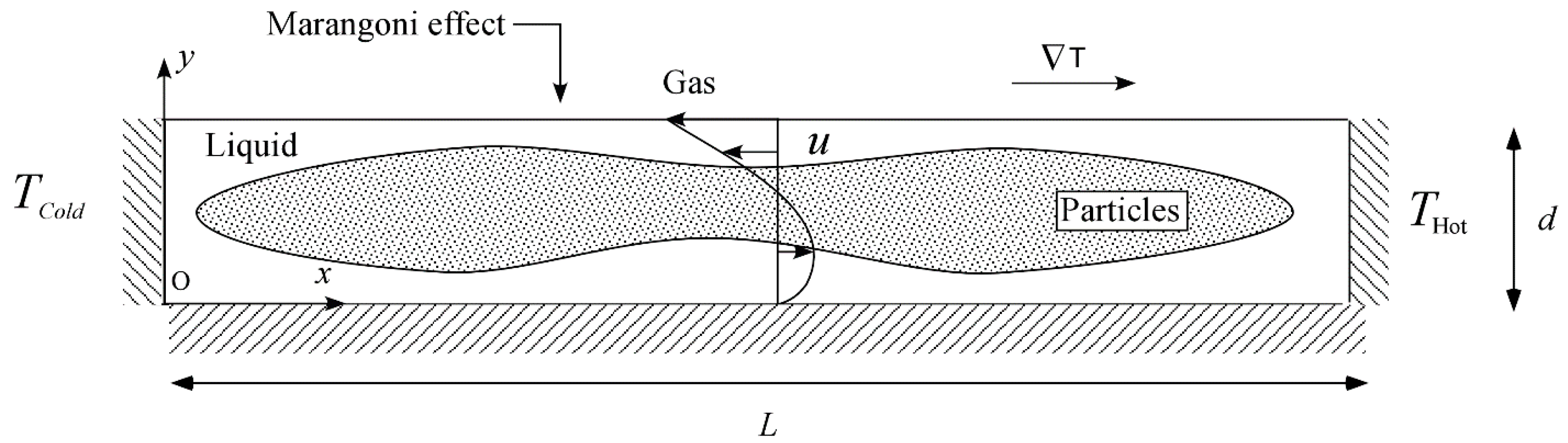
where V= 0 implies u = v = 0, i.e., the liquid is motionless with a linear temperature profile along the x coordinate (the temperature is TCold = 0 on the cold sidewall and THot = 1 on the other side).
t = 0: V(x,y) = 0, T(x,y) = x/A
Adiabatic conditions are assumed for both the free liquid–gas interface and the bottom wall. Accordingly, the thermal and kinematic boundary conditions for t > 0 read:
where Ma is the Marangoni number defined as Ma = σTΔTd/μα (where σT is the surface tension derivative with respect to temperature).
u = 0, v = 0 and T = 0 at x = 0 (left wall)
u = 0, v = 0 and T = 1 at x = A (right wall)
u = 0, v = 0, and ∂T/∂y = 0 at y = 0 (bottom wall)
v = 0, ∂u/∂y = −Ma∂T/∂x, and ∂T/∂y = 0 at y = 1 (free surface)
Solid particles are seeded in the domain when the hydrothermal wave has reached its asymptotic state in terms of amplitude and frequency (particles being distributed uniformly and with velocity and temperature initially equal to those of the fluid).
2.6. The Numerical Method
As the solution technique we have implemented a projection method for incompressible fluid flow based on the use of primitive variables (namely, velocity, pressure and temperature; see, e.g., Lappa [40] for an exhaustive description). Here we limit ourselves to reporting that this method relies on an intermediate step where the momentum equation is integrated in time disregarding the pressure gradient. In a second stage, an elliptic (Poisson) equation, formally obtained by substituting a ‘corrected’ velocity in the continuity equation, is solved iteratively (the corrected velocity being expressed as a linear combination of the intermediate velocity and the pressure gradient). This provides the required value of the pressure needed to close the problem from a mathematical point of view.
In particular, this numerical approach has been implemented here using schemes explicit in time and standard central differences for the convective and diffusive terms appearing in both Equations (16) and (18). The coupling between pressure and velocity has been reinforced through the adoption of a staggered grid arrangement.
Similarly, an explicit in time (4th order Runge–Kutta) scheme has been employed to integrate Equations (17) and (19). The fluid velocity and temperature at the generic particle location appearing in these equations have been determined at each time step starting from nodal values on the staggered grid and using simple linear interpolations.
A relevant validation of both these Eulerian and Lagrangian kernels can be found in [15] and [28], respectively. In particular, the following benchmark cases were considered in this regard: the HTW originally examined by Xu and Zebib [13] for pure Marangoni flow in a rectangular cavity with A = 20, Pr = 10 and Ma = 1.05 × 10⁴ (for which we obtained an angular frequency ω ≅ 36 matching with an approximation of %2 the value 35.17 reported by these authors) and the particle accumulation structures emerging in a liquid bridge with aspect ratio (height/diameter) A = 0.34, Pr = 8, Ma = 20,600 and particle density ratio ξ = 1.85 originally investigated numerically by Melnikov et al. [46] (obtaining an excellent agreement with regard to the topology of the emerging particle structures, see Figure 2 in [28], and in terms of the emerging HTW, i.e., an angular frequency of 71.4 against the reference value 73.3).
The outcomes of the mesh refinement study conducted for the present case using uniform structured grids (assuming the same aspect ratio and Marangoni number considered in Section 3) are summarized in Table 1.
As quantitatively substantiated by the data reported in this table, mesh independence has been achieved with 30 points per unit non-dimensional length.
3. Results
In order to extend the earlier results by Lappa [15] for pure Marangoni flow and no particles, the following conditions are considered: Pr = 15 (see Table 2 for the related fluid properties), Ma = 2 × 10⁴ and A = 20 (see Figure 1). Moreover, the following ranges are examined in terms of particle Stokes number and mass load: 10−6 ≤ St ≤ 10−5, 0 ≤ χ ≤ 0.7. Particles are assumed to be made of tungsten (Table 3), which makes the corresponding volume fraction span the interval 0 ≤ φ ≤ 2.8 × 10⁻² (as in [40]).
For the convenience of the reader, we start the analysis of the numerical results from the simplest possible situation, namely, the development of the HTW in the absence of dispersed particles (i.e., χ = 0, see Section 3.1).
3.1. Particle-Free Dynamics
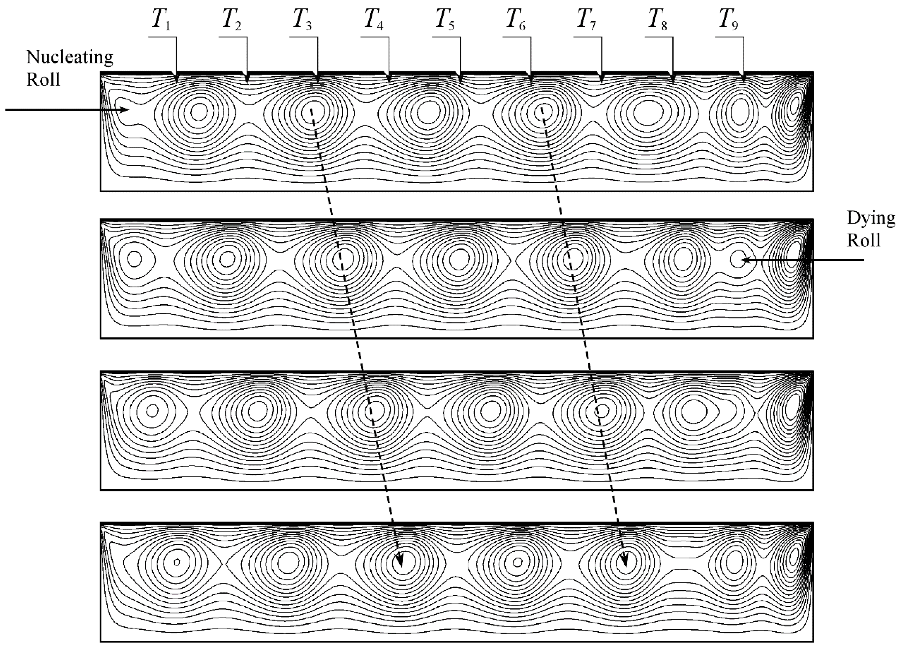
The reader may get a first glimpse of the patterning behavior of such a system by taking a look at Figure 2, where snapshots of the ‘typical’ flow structure produced by a two-dimensional simulation of the HTW have been reported in an ordered fashion. It can be seen that, with the exception of a vortex steadily located in proximity to the hot side, the wave manifests itself as a disturbance spreading continuously in the upstream direction in the form of a sequence of rolls (moving in a direction opposite to the surface flow, which in the figure is directed from the right hot side towards the left cold side). The rolls nucleate at the cold side (as indicated by the horizontal arrow in the first snapshot) and then travel towards the hot side, maintaining the same sense of circulation as the main circulation system in which they are embedded (anti-clockwise rotation in Figure 2).
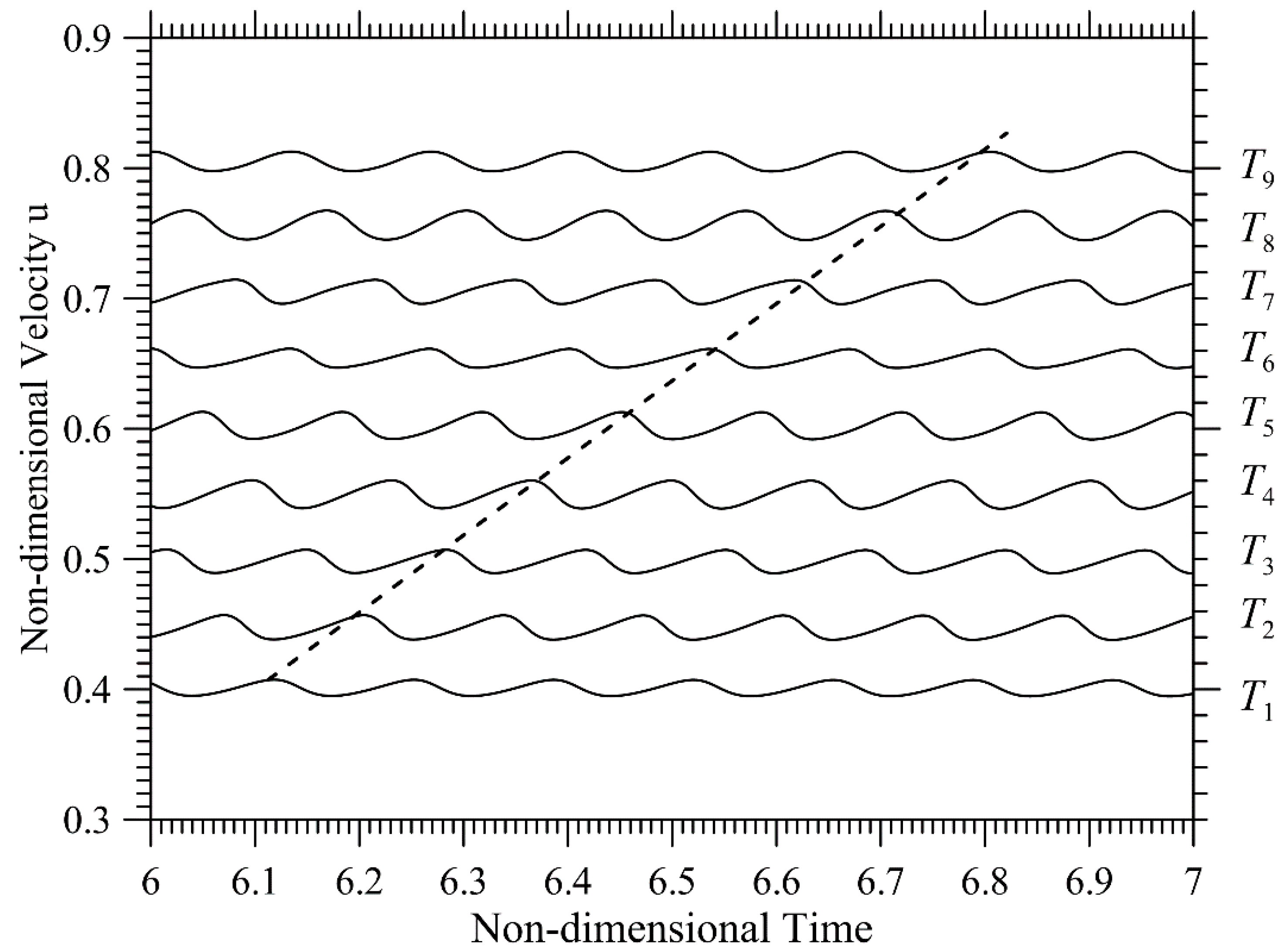
The continuous displacement of rolls from one side of the cavity to the other side (where they die) produces a time-periodic distortion in the temperature field, which can be measured by means of ‘numerical’ probes evenly spaced along the horizontal direction (as shown in Figure 3). The essentially traveling nature of the fluid-dynamic disturbance can be appreciated in this figure by evaluating the phase shift among different signals (shift increasing linearly with the horizontal distance between the two considered thermocouples).
The addition of particles to this fluid-dynamic system leads to two subjects running in parallel, both deserving investigation, i.e., the patterning phenomena produced by the interaction of particles with the traveling wave (Section 3.2) and the back influence that particles exert on the properties of the wave itself (Section 3.3). Both subjects, of course, display sensitivity to the properties and amount of the dispersed solid mass (particle size and mass loading).
Along these lines, we should recall that particles are expected to influence the background flow (the hydrothermal wave) essentially through two different mechanisms: one related to the finite mass of each particle, physically depending on the different densities of the considered two phases and scaling with the total amount of solid mass physically present in the fluid domain (as measured by the non-dimensional parameter χ), and the other of a purely ‘viscous’ origin (due to the ‘friction’ between the particles and the liquid, therefore depending on the particle Stokes number St and their overall number).
As outlined at the beginning of Section 3, the material considered for the particles is tungsten (for which ξ = 24 and ζ = 0.063). Having fixed the liquid (silicone oil) and the solid (tungsten), we naturally assume χ and St as the main degrees of freedom of the considered problem (given their expected impact on the properties of the HTW in relation to the inertial and drag responses of the dispersed matter).
Before embarking onto the description of the related results, it is worth remarking that, with the present choice of parameters, the three criteria represented by Equations (21), (31) and (32) about the conditions to be satisfied to make the overall mathematical and numerical approach applicable (well-posed) are all largely met with St, ϕ and φ being much smaller than unity. For the considered conditions and mesh, indeed, 8.5 × 10⁻⁴ ≤ ϕ ≤ 8.5 × 10⁻² and 4.2 × 10⁻³ ≤ φ ≤ 2.8 × 10⁻².
3.2. Patterning Behavior
As explained in Section 2.6, the considered flow is incompressible, which means that the volume of fluid parcels is conserved in time. The peculiar properties of particles motion, however, allow them (their velocity field) to escape this constraint. Indeed, even though the divergence of the fluid velocity field is zero (Equation (15)), the finite size and mass of the considered particles can cause compressibility effects in the particle velocity field.
An almost immediate realization of the compressible nature of particle motion can be obtained by applying the divergence operator to Equation (17):
In turn, the effects, due to the non-solenoidal nature of the Vp (), can manifest in the form of depletion of dispersed solid matter occurring in some regions of the physical domain, and/or as accumulation phenomena in others (such events, generally known as preferential concentration, typically lead to the formation of sub-domains with varying particle concentrations such as banded patterns or localized or extended particle clusters encapsulated in wider areas of clear fluid; see, e.g., Sapsis and Haller [47]).
For the case of flows in normal gravity conditions, there is a vast amount of literature on this subject for particles interacting with laminar or turbulent background flows, relevant examples being represented by the works of Raju and Meiburg [48,49], Dávila and Hunt [50], Eames and Gilbertson [51], Chen et al. [52], Ravichandran et al. [53] and Bergougnoux et al. [54]. Other efforts (Yarin et al. [55], Gan et al. [56], Akbar et al. [57], Puragliesi et al. [58], Haeri and Shrimpton [59], Xu et al. [60]) have expressly considered non-isothermal conditions (leading to thermal buoyancy convection). These studies have provided evidence that, even in the presence of particle inertia and gravity, some conditions can be identified, for which near-equilibrium particle recirculation zones are maintained by thermal convection (particles being allowed to remain suspended in these regions in certain ranges of the Stokes number and the Rayleigh number).
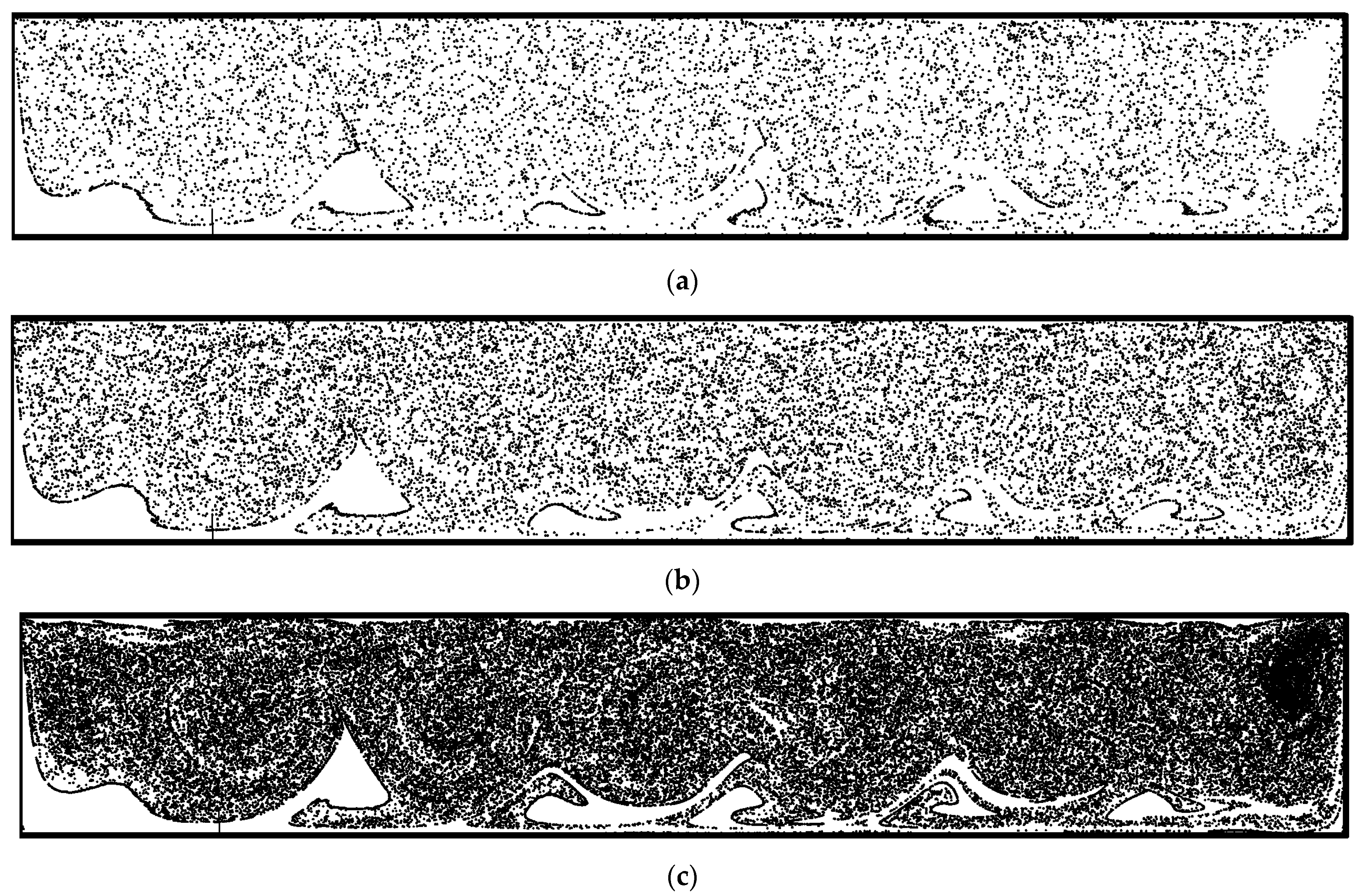
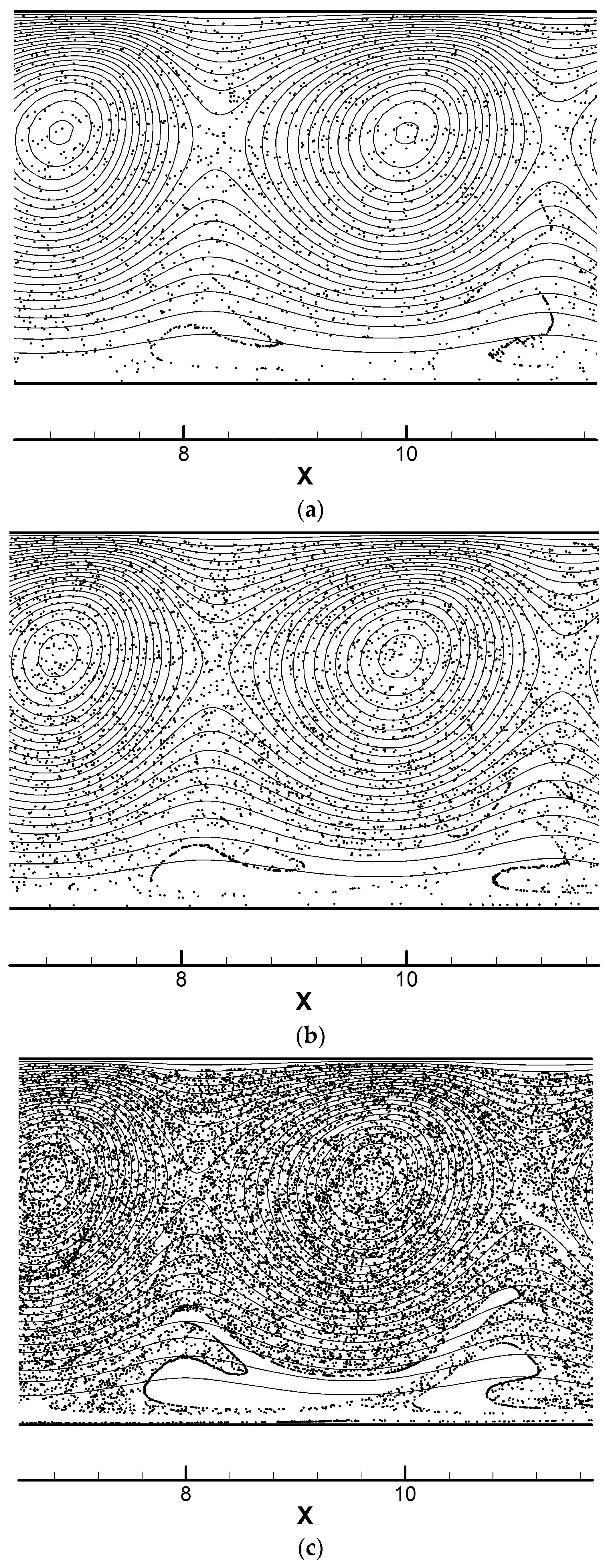
In the present case, gravity is absent (as we assume the considered system to be in microgravity conditions). Hence, any processes that depend on gravity are excluded, and the present situation may be regarded as a particularly suitable testbed for the assessment and detailed analysis of the role of particle-fluid inertial effects. Along these lines, some initial insights can be obtained by taking a look at Figure 4, where the particle distribution associated with the traveling rolls produced by the instability of the Marangoni flow (HTW) has been reported for a fixed value of the mass loading and different values of the particle Stokes number.
As a fleeting glimpse into this figure would confirm, the Stokes number has an appreciable influence on the distribution of particles. In particular, meaningful insights follow naturally from a comparison of Figure 4a with Figure 4c (please note that, for illustration purposes, in these figures the depth of the fluid layer is three times its real dimension). Such effects are evident especially in the vortex being steadily attached to the hot wall (right side). The strong vorticity being available there causes a centrifugal force, which can cause the ejection of particles from the core of the vortex if their mass is sufficiently high. This is actually what can be seen in Figure 4a; a spot of clear (particle free) fluid is formed in the center of this vortex for St = 10−5. As St is decreased, however, the size of the clear spot decreases progressively until it is no longer visible for St = 10−6.
Notably, the formation of this clear spot is not a feature of the other rolls pertaining to the HTW even if the highest value of St is considered, which requires a proper interpretation.
As qualitatively made evident by Figure 5, a tendency is still present to eject particles and let them accumulate along particle-dense lines located at the periphery of the rolls, which display some similarities with the analogous phenomena reported by Lappa [61] for the case of rising (unsteady) thermal plumes of a buoyant nature interacting with non-isodense particles. In that study, particle-accumulation loci having the shape of distorted closed circuits were found in the lobes of the plume cap as a result of the vorticity concentrated in those regions, which can propel particles along curved (closed in many circumstances) trajectories.
In the present case, closed ‘loops’ or circuits of particles are not formed, and an explanation/justification for this trend can be elaborated in its simplest form on the basis of the argument that the flow consists of a ‘series’ of rolls. The particle-ejecting vortices do not occupy fixed positions in space (as time progresses these vortices travel towards the hot side). This means that as time passes, the particle-dense lines formed by one roll at its periphery due to the centrifugal effects described above are subjected to other influential factors (essentially of a convective nature).
In particular, a more involved justification of this process requires recalling that, as an intrinsic feature of HTWs, the rolls traveling in the upstream direction (from the cold side to the hot side) do not result in a net transport of fluid in the same direction (the propagation of the disturbance is not associated with the physical displacement of fluid in the same direction of the wave). This means that, unlike the case of a plume of buoyant nature transporting fluid, in the present case a particle circuit formed by one roll will not be able to follow the roll in its migration journey along the spatial extension of the layer. This, in turn, implies that after a certain time such a circuit will be subjected to the disturbing action exerted on it by the next roll travelling from the cold side to the hot wall. Obviously, the particle circuit will also feel the effect of the surface fluid and of the return flow, which tend to stretch it in the direction of the applied temperature gradient.
All these effects contribute to prevent the formation of permanent accumulation circuits (closed particle-dense lines) in the domain. Circuits potentially formed by centrifugal effects are progressively distorted and finally broken (especially for higher values of the Stokes number), leading to the apparently random distribution in the flow of parts or segments resulting from the just discussed circuit rupture events.
The formation of circuits spanning the entire extension of the physical domain, such as those emerging in the case of liquid bridges [23,24,25,26,27,28,29,30,31,32,33,34,35,36,37,38,39], is also prevented because finite-size rectangular containers lack the necessary feedback mechanisms which allow particle self-organization. The closed streamtubes playing the role of templates for the accumulation of particles in the liquid bridge do not exist in the present case. In liquid bridges they are made possible by the ‘periodic nature’ of the domain in the circumferential direction. In the present case the wave is continuously generated at the cold side (where rolls nucleate) and dies at the opposite size (where rolls are suppressed).
Due to the joint action exerted by all the vortices on the solid mass distributed in the fluid (propelling particles from the center of rolls in the outward direction) and the intense descending flow located in proximity to the cold boundary that tends to set a distance between particles and this wall, particles simply tend to be accumulated (as time increases) along the lower periphery of the main circulation system. As a result of this mechanism, a wavy boundary, separating the upper particle-rich area from a relatively depleted area lying on the bottom, is formed.
As shown by the simulations, the spatial sinusoidal modulations visible in the shape of this boundary travel in the same direction of the wave, which is also in the direction of the return flow (from the hot to the cold wall). Such modulations or distortions appear in the form of patches of clear fluid protruding into the particle-dense region in the limited portion of space separating consecutive rolls. This evolution is the result of the interplay of the different velocities of the travelling wave and the return flow.
3.3. Inertial Effects and Wave Propagation
The key aim of this section is to introduce some predictive links between the properties of the resulting wave and those of the particles and discuss critically the fundamental mechanism by which energy is channeled from the fluid into the particles (or vice versa).
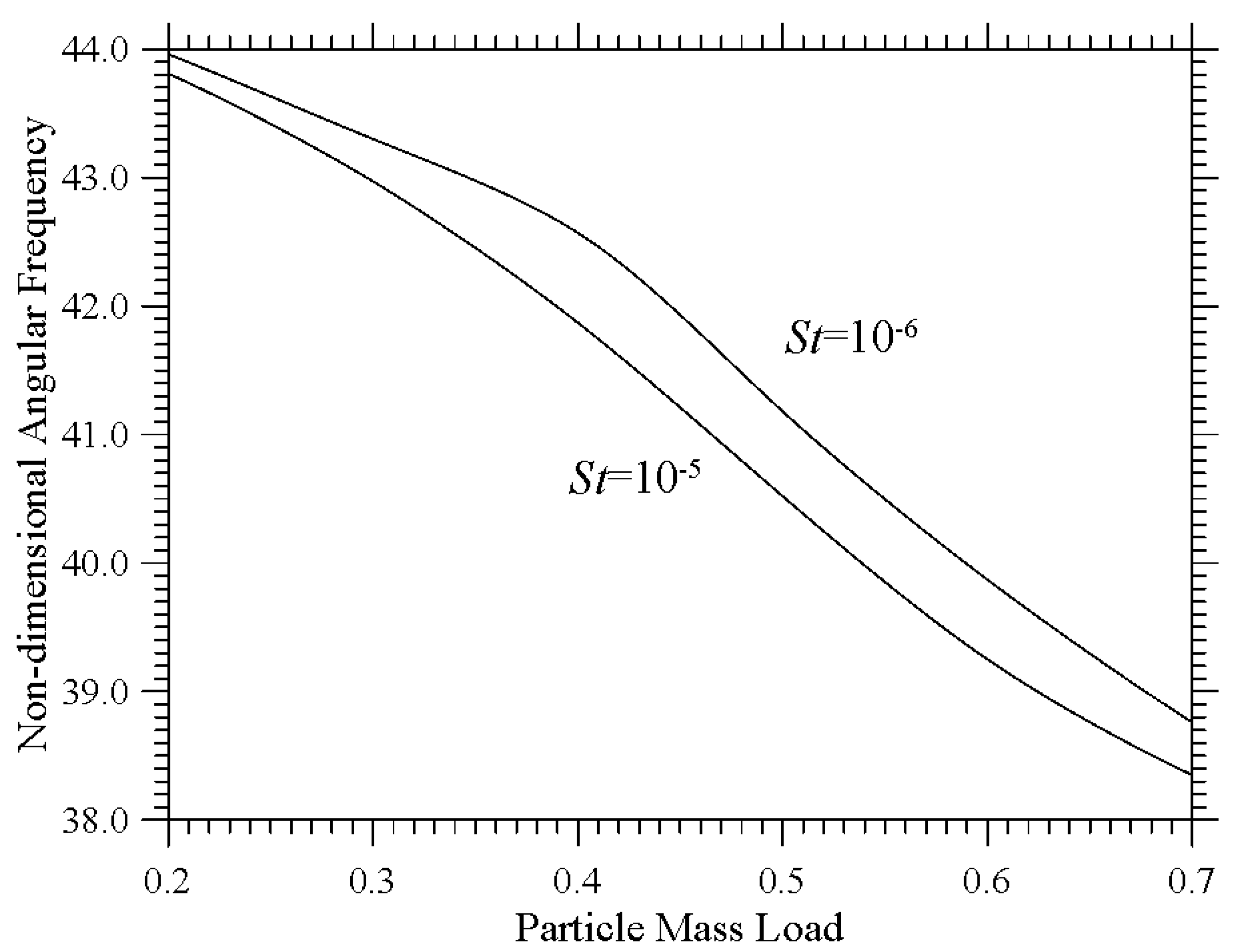
Along these lines, Figure 6 reveals the increasing attenuation of the angular velocity of propagation of the HTW that can be obtained for a fixed value of the particle radius when the mass load is increased (a variation of 14% for χ increasing from 0.2 to 0.7).
This figure also provides some evidence for the role of the viscous interactions between the liquid and the particles. While the inertial effects related to the density mismatch are expected to depend globally on the total amount of solid mass physically added to the fluid system, the influence of the viscous interactions is much more subtle because it is connected to the overall number of particles and their effective radius. As quantitatively substantiated by this figure, however, in the present case, the dependence of the wave angular frequency on the Stokes number seems to be relatively limited (the induced percentage variation is less than 3%).
To elucidate further the significance of this observation, one may consider known analogous dynamics for high-speed regimes, such as those related to the interaction of a shock wave with a dusty gas (Lappa et al. [43]). For high fluid velocities (high values of the Reynolds number), in general, the viscous contribution appearing in Equation (17) plays a dominant role because of the large velocity difference between fluid and particles. Since in the present case, such a difference is relatively small, the particle-finite-mass-related effects should be expected to be much more important in the mechanism responsible for the exchange of momentum between the fluid and the particles. Indeed, this is what can be inferred from Figure 6.
In turn, the scarce influence of St on the HTW property for a fixed χ may be ascribed to the fact that for given values of the mass load and density ratio, the overall solid surface exposed to fluid flow (summation of all particle surfaces) does not change. Indeed, such a quantity (normalized by the domain area) can be expressed as
which, taking into account Equation (24), can be recast as
This supports the observation that the momentum exchange between the particles and the fluid due to particle drag effects is almost independent from the Stokes number. A similar concept also holds for the exchanges occurring in terms of thermal energy (heat). These are expected to scale (for a fixed mass load) with the overall solid surface exposed to fluid flow and, therefore, again with the parameter . In any case, as a concluding remark for this section, we wish to highlight that this effect can be considered almost negligible. Indeed, simulations repeated after disabling the solution of Equation (19) have revealed no significant changes in terms of hydrothermal disturbance propagation velocity. Among other things, this is in line with the conclusions that could be drawn by considering arguments based on the ‘heat capacity’ of each phase. This property can be expressed as the product of the considered phase specific heat coefficient and mass. Accordingly, the ratio of these capacities for the solid and liquid phases simply reads
In the present case ζ = 0.063, and assuming the worst case in terms of χ, one would get Hc = O(10−2) << 1. As this ratio can be seen as a measure of the thermal inertia of the dispersed phase, i.e., the degree of slowness with which the temperature of the particles reaches that of the surroundings or, in an equivalent way, as the capacity of the solid mass to store heat and to delay its transmission, it can be concluded that the solid phase can be considered in thermal equilibrium with the liquid one (i.e., at the same temperature).
4. Conclusions
A focused analysis of the phenomenon related to the emergence and propagation of hydrothermal waves in Marangoni flows has been conducted in a situation for which the considered fluid is a mixture of oil and solid particles having a density significantly larger than that of the carrier fluid. Although the particle volume fraction has been limited to situations for which the assumption of non-interacting particles can still be considered valid, values of the mass load have been examined for which the back influence of the dispersed solid mass on fluid flow is not negligible.
It has been found that, on increasing the mass load, the velocity of propagation of the hydrothermal disturbances undergoes shrinkage, while it displays a weak sensitivity to the particle Stokes number. This indicates that the two phases are coupled within an interlocking ensemble of mutual interferences, where while frictional effects play an important role in determining the transfer of momentum from the fluid to the particles, the back influence of particles on the hydrothermal wave is exerted primarily through inertial effects stemming from the different densities of the two phases. Moreover, in such a hierarchy of interactions, the tertiary influence represented by heat exchange effects can be considered negligible.
The lack of particle accumulation structures similar to those observed in the case of liquid bridges has been justified considering that, as a result of the multicellular nature of the HTW and geometrical constraints due to the rectangular shape of the container, the tendency of this system to form particle-dense lines due to inertial effects is hindered.
An exciting prospect for the future is to extend these studies to the case of three-dimensional configurations in order to determine the influence of the dispersed phase on the angle of propagation of the HTW with respect to the direction of the imposed temperature gradient.
Funding
This work was supported by the U.K. Engineering and Physical Sciences Research Council (EPSRC grant EP/R043167/1) and the U.K. Space Agency in the framework of the JEREMI (Japanese European Research Experiments on Marangoni Instabilities) ESA-JAXA project.
Institutional Review Board Statement
Not applicable.
Informed Consent Statement
Not applicable.
Data Availability Statement
Publicly available datasets are made available with this study. These data can be found in the pure repository of the University of Strathclyde; https://0-doi-org.brum.beds.ac.uk/10.15129/9f4d022e-dfd8-4d58-a2ec-72c322803598.
Conflicts of Interest
The author declares no conflict of interest.
Abbreviations
| Nomenclature | |
| A | Aspect ratio |
| C | Specific heat |
| d | Layer thickness |
| h | Heat convective transfer coefficient |
| m | Particle mass |
| Ma | Marangoni number |
| N | Number of particles |
| p | Pressure |
| Pr | Prandtl number |
| R | Particle radius |
| Re | Reynolds number |
| S | Interphase exchange term |
| St | Particle Stokes number |
| T | Temperature |
| t | Time |
| u | Velocity component along x |
| V | Velocity |
| v | Velocity component along y |
| x | Horizontal coordinate |
| y | Vertical coordinate |
| Greek Symbols | |
| λ | Thermal conductivity |
| ω | Angular frequency |
| Ω | Area |
| ξ | Density ratio |
| μ | Dynamic viscosity |
| ρ | Fluid density |
| ν | Kinematic viscosity |
| χ | Mass load |
| ϕ | Particle to computational cell volume ratio |
| τ | Relaxation time |
| ζ | Specific heat ratio |
| ψ | Stream function |
| α | Thermal diffusivity |
| φ | Particles volume fraction |
| ΔΤ | Temperature difference |
| Subscripts | |
| E | Energy |
| HTW | Hydrothermal wave |
| m | Momentum |
| p | Particle or pressure |
| v | Volume |
| Superscripts | |
| s | Solid phase |
References
- Schwabe, D.; Scharmann, A. Some evidence for the existence and magnitude of a critical Marangoni number for the onset of oscillatory flow in crystal growth melts. J. Cryst. Growth 1979, 46, 125–131. [Google Scholar] [CrossRef]
- Smith, M.K.; Davis, S.H. Instabilities of dynamic thermocapillary liquid layers. Part 1: Convective instabilities. J. Fluid Mech. 1983, 132, 119–144. [Google Scholar] [CrossRef]
- Priede, J.; Gerbeth, G. Convective, absolute, and global instabilities of thermocapillary-buoyancy convection in extended layers. Phys. Rev. E 1997, 56, 4187–4199. [Google Scholar] [CrossRef]
- Daviaud, F.; Vince, J.M. Traveling waves in a fluid layer subjected to a horizontal temperature gradient. Phys. Rev. E 1993, 48, 4432–4436. [Google Scholar] [CrossRef] [PubMed] [Green Version]
- Gillon, P.; Homsy, G.M. Combined thermocapillary-buoyancy convection in a cavity: An experimental study. Phys. Fluids 1996, 8, 2953–2963. [Google Scholar] [CrossRef]
- De Saedeleer, C.; Garcimartin, A.; Chavepeyer, G.; Platten, J.K.; Lebon, G. The instability of a liquid layer heated from the side when the upper surface is open to air. Phys. Fluids 1996, 8, 670–676. [Google Scholar] [CrossRef] [Green Version]
- Garcimartìn, A.; Mukolobwiez, N.; Daviaud, F. Origin of surface waves in surface tension driven convection. Phys. Rev. E 1997, 56, 1699–1705. [Google Scholar] [CrossRef] [Green Version]
- Pelacho, M.A.; Burguete, J. Temperature oscillations of hydrothermal waves in thermocapillary-buoyancy convection. Phys. Rev. E 1999, 59, 835–840. [Google Scholar] [CrossRef] [Green Version]
- Pelacho, M.A.; Garcimartın, A.; Burguete, J. Local Marangoni number at the onset of hydrothermal waves. Phys. Rev. E 2000, 62, 477–483. [Google Scholar] [CrossRef] [Green Version]
- Burguete, J.; Mukolobwiez, N.; Daviaud, N.; Garnier, N.; Chiffaudel, A. Buoyant-thermocapillary instabilities in extended liquid layers subjected to a horizontal temperature gradient. Phys. Fluids 2001, 13, 2773–2787. [Google Scholar] [CrossRef] [Green Version]
- Pelacho, M.A.; Garcimartin, A.; Burguete, J. Travel Instabilities in Lateral Heating. Int. J. Bifurc. Chaos 2001, 11, 2881–2886. [Google Scholar] [CrossRef]
- Peltier, L.; Biringen, S. Time-dependent thermocapillary convection in a rectangular cavity: Numerical results for a moderate Prandtl number fluid. J. Fluid Mech. 1993, 257, 339–357. [Google Scholar] [CrossRef]
- Xu, J.; Zebib, A. Oscillatory two- and three-dimensional thermocapillary convection. J. Fluid Mech. 1998, 364, 187–209. [Google Scholar] [CrossRef]
- Tang, Z.M.; Hu, W.R. Hydrothermal Wave in a Shallow Liquid Layer. Microgravity Sci. Technol. 2005, 16, 253–258. [Google Scholar] [CrossRef]
- Lappa, M. Hydrothermal waves in two-dimensional liquid layers with sudden changes in the available cross-section. Int. J. Numer. Methods Heat Fluid Flow 2017, 27, 2629–2649. [Google Scholar] [CrossRef] [Green Version]
- Parmentier, P.M.; Regnier, V.C.; Lebon, G. Buoyant-thermocapillary instabilities in medium-Prandtl number fluid layers subject to a horizontal temperature gradient. Int. J. Heat Mass Transf. 1993, 36, 2417–2427. [Google Scholar] [CrossRef]
- Lappa, M. Patterning behaviour of gravitationally modulated supercritical Marangoni flow in liquid layers. Phys. Rev. E 2016, 93, 053107. [Google Scholar] [CrossRef] [Green Version]
- Shevtsova, V.; Mialdun, A.; Kawamura, H.; Ueno, I.; Nishino, K.; Lappa, M. The JEREMI-Project on Thermocapillary Convection in Liquid Bridges. Part B: Impact of Co-axial Gas Flow. Fluid Dyn. Mater. Process. 2014, 10, 197–240. [Google Scholar]
- Lappa, M. On the Formation and Propagation of Hydrothermal waves in Solidifying Liquid Layers. Comput. Fluids 2018, 172, 741–760. [Google Scholar] [CrossRef] [Green Version]
- Salgado Sanchez, P.; Porter, J.; Ezquerro, J.M.; Tinao, I.; Laverón-Simavilla, A. Pattern selection for thermocapillary flow in rectangular containers in microgravity. Phys. Rev. Fluids 2022, 7, 053502. [Google Scholar] [CrossRef]
- Ospennikov, N.A.; Schwabe, D. Thermocapillary flow without return flow–linear flow. Exp. Fluids 2004, 36, 938–945. [Google Scholar] [CrossRef]
- Schwabe, D.; Hintz, P.; Frank, S. New Features of Thermocapillary Convection in Floating Zones Revealed by Tracer Particle Accumulation Structures. Microgravity Sci. Technol. 1996, 9, 163–168. [Google Scholar]
- Schwabe, D.; Mizev, A.I.; Udhayasankar, M.; Tanaka, S. Formation of dynamic particle accumulation structures in oscillatory thermocapillary flow in liquid bridges. Phys. Fluids 2007, 19, 072102. [Google Scholar] [CrossRef]
- Schwabe, D.; Mizev, A.I. Particles of different density in thermocapillary liquid bridges under the action of travelling and standing hydrothermal waves. Eur. Phys. J. Spec. Top. 2011, 192, 13–27. [Google Scholar] [CrossRef]
- Pushkin, D.; Melnikov, D.; Shevtsova, V. Ordering of Small Particles in One-Dimensional Coherent Structures by Time-Periodic Flows. Phys. Rev. Lett. 2011, 106, 234501. [Google Scholar] [CrossRef] [PubMed] [Green Version]
- Melnikov, D.E.; Pushkin, D.O.; Shevtsova, V.M. Synchronization of finite-size particles by a traveling wave in a cylindrical flow. Phys. Fluids 2013, 25, 092108. [Google Scholar] [CrossRef]
- Lappa, M. Assessment of the role of axial vorticity in the formation of Particle Accumulation Structures (PAS) in supercritical Marangoni and hybrid thermocapillary-rotation-driven flows. Phys. Fluids 2013, 25, 012101. [Google Scholar] [CrossRef] [Green Version]
- Lappa, M. On the variety of particle accumulation structures under the effect of gjitters. J. Fluid Mech. 2013, 726, 160–195. [Google Scholar] [CrossRef] [Green Version]
- Lappa, M. On the Existence and Multiplicity of One-dimensional Solid Particle Attractors in Time-dependent Rayleigh-Bénard Convection. Chaos 2013, 23, 013105. [Google Scholar] [CrossRef] [Green Version]
- Lappa, M. Stationary Solid Particle Attractors in Standing Waves. Phys. Fluids 2014, 26, 013305. [Google Scholar] [CrossRef] [Green Version]
- Kuhlmann, H.C.; Lappa, M.; Melnikov, D.; Mukin, R.; Muldoon, F.H.; Pushkin, D.; Shevtsova, V.S.; Ueno, I. The JEREMI-Project on thermocapillary convection in liquid bridges. Part A: Overview of Particle Accumulation Structures. Fluid Dyn. Mater. Process. 2014, 10, 1–36. [Google Scholar] [CrossRef]
- Gotoda, M.; Melnikov, D.E.; Ueno, I.; Shevtsova, V. Experimental study on dynamics of coherent structures formed by inertial solid, particles in three-dimensional periodic flows. Chaos 2016, 26, 073106. [Google Scholar] [CrossRef] [PubMed]
- Gotoda, M.; Sano, T.; Kaneko, T.; Ueno, I. Evaluation of existence region and formation time of particle accumulation structure (PAS) in half-zone liquid bridge. Eur. Phys. J. Spec. Top. 2015, 224, 299. [Google Scholar] [CrossRef]
- Lappa, M. On the nature, formation and diversity of particulate coherent structures in Microgravity Conditions and their relevance to materials science and problems of Astrophysical interest. Geophys. Astrophys. Fluid Dyn. 2016, 110, 348–386. [Google Scholar] [CrossRef] [Green Version]
- Melnikov, D.E.; Shevtsova, V. Different types of Lagrangian coherent structures formed by solid particles in three-dimensional time-periodic flows. Eur. Phys. J. Spec. Top. 2017, 226, 1239–1251. [Google Scholar] [CrossRef]
- Capobianchi, P.; Lappa, M. Particle accumulation structures in noncylindrical liquid bridges under microgravity conditions. Phys. Rev. Fluids 2020, 5, 084304. [Google Scholar] [CrossRef]
- Capobianchi, P.; Lappa, M. On the influence of gravity on particle accumulation structures in high aspect-ratio liquid bridges. J. Fluid Mech. 2021, 908, A29. [Google Scholar] [CrossRef]
- Capobianchi, P.; Lappa, M. Particle accumulation structures in a 5 cSt silicone oil liquid bridge: New data for the preparation of the JEREMI Experiment. Microgravity Sci. Technol. 2021, 33, 31. [Google Scholar] [CrossRef]
- Sakata, T.; Terasaki, S.; Saito, H.; Fujimoto, S.; Ueno, I.; Yano, T.; Nishino, K.; Kamotani, Y.; Matsumoto, S. Coherent structures of m = 1 by low-Stokes-number particles suspended in a half-zone liquid bridge of high aspect ratio: Microgravity and terrestrial experiments. Phys. Rev. Fluids 2021, 7, 014005. [Google Scholar] [CrossRef]
- Lappa, M. Characterization of two-way coupled thermovibrationally driven particle attractee. Phys. Fluids 2022, 34, 053109. [Google Scholar] [CrossRef]
- Maxey, M.R.; Riley, J.J. Equation of motion for a small rigid sphere in a nonuniform flow. Phys. Fluids 1983, 26, 883–889. [Google Scholar] [CrossRef]
- Bianco, V.; Chiacchio, F.; Manca, O.; Nardini, S. Numerical investigation of nanofluids forced convection in circular tubes. Appl. Therm. Eng. 2009, 29, 3632–3642. [Google Scholar] [CrossRef] [Green Version]
- Lappa, M.; Drikakis, D.; Kokkinakis, I. On the propagation and multiple reflections of a blast wave travelling through a dusty gas in a closed box. Phys. Fluids 2017, 29, 033301. [Google Scholar] [CrossRef] [Green Version]
- Ranz, W.E.; Marshall, W.R., Jr. Evaporation from Drops, Part I. Chem. Eng. Prog. 1952, 48, 141–146. [Google Scholar]
- Greifzu, F.; Kratzsch, C.; Forgber, T.; Lindner, F.; Schwarze, R. Assessment of particle-tracking models for dispersed particle-laden flows implemented in OpenFOAM and ANSYS FLUENT. Eng. Appl. Comput. Fluid Mech. 2016, 10, 30–43. [Google Scholar] [CrossRef] [Green Version]
- Melnikov, D.E.; Pushkin, D.O.; Shevtsova, V.M. Accumulation of particles in time-dependent thermocapillary flow in a liquid bridge. Modeling of experiments. Eur. Phys. J. Spec. Top. 2011, 192, 29–39. [Google Scholar] [CrossRef] [Green Version]
- Sapsis, T.; Haller, G. Clustering criterion for inertial particles in two-dimensional time-periodic and three-dimensional steady flows. Chaos 2010, 20, 017515. [Google Scholar] [CrossRef]
- Raju, N.; Meiburg, E. The accumulation and dispersion of heavy particles in forced two-dimensional mixing layers. Part 2: The effect of gravity. Phys. Fluids 1995, 7, 1241–1264. [Google Scholar] [CrossRef] [Green Version]
- Raju, N.; Meiburg, E. Dynamics of small spherical particles in vortical and stagnation point flow fields. Phys. Fluids 1997, 9, 299–314. [Google Scholar] [CrossRef]
- Dávila, J.; Hunt, J.C.R. Settling of small particles near vortices and in turbulence. J. Fluid Mech. 2001, 440, 117–145. [Google Scholar] [CrossRef]
- Eames, I.; Gilbertson, M.A. The settling and dispersion of small dense particles by spherical vortices. J. Fluid Mech. 2004, 498, 183–203. [Google Scholar] [CrossRef] [Green Version]
- Chen, L.; Goto, S.; Vassilicos, J.C. Turbulent clustering of stagnation points and inertial particles. J. Fluid Mech. 2006, 553, 143–154. [Google Scholar] [CrossRef] [Green Version]
- Ravichandran, S.; Perlekar, P.; Govindarajan, R. Attracting fixed points for heavy particles in the vicinity of a vortex pair. Phys. Fluids 2014, 26, 013303. [Google Scholar] [CrossRef] [Green Version]
- Bergougnoux, L.; Bouchet, G.; Lopez, D.; Guazzelli, E. The motion of solid spherical particles falling in a cellular flow field at low Stokes number. Phys. Fluids 2014, 26, 093302. [Google Scholar] [CrossRef] [Green Version]
- Yarin, A.L.; Kowalewski, T.A.; Hiller, W.J.; Koch, S. Distribution of particles suspended in convective flow in differentially heated cavity. Phys. Fluids 1996, 8, 1130. [Google Scholar] [CrossRef] [Green Version]
- Gan, H.; Chang, J.; Feng, J.J.; Hu, H.H. Direct numerical simulation of the sedimentation of solid particles with thermal convection. J. Fluid Mech. 2003, 481, 385–411. [Google Scholar] [CrossRef] [Green Version]
- Akbar, M.K.; Rahman, M.; Ghiaasiaan, S.M. Particle transport in a small square enclosure in laminar natural convection. J. Aerosol Sci. 2009, 40, 747–761. [Google Scholar] [CrossRef]
- Puragliesi, R.; Dehbi, A.; Leriche, E.; Soldati, A.; Deville, M. DNS of buoyancy-driven flows and Lagrangian particle tracking in a square cavity at high Rayleigh numbers. Int. J. Heat Fluid Flow 2011, 32, 915–931. [Google Scholar] [CrossRef]
- Haeri, S.; Shrimpton, J.S. Fully resolved simulation of particle deposition and heat transfer in a differentially heated cavity. Int. J. Heat Fluid Flow 2014, 50, 1–15. [Google Scholar] [CrossRef] [Green Version]
- Xu, A.; Tao, S.; Shi, L.; Xi, H.D. Transport and deposition of dilute microparticles in turbulent thermal convection. Phys. Fluids 2020, 32, 083301. [Google Scholar] [CrossRef]
- Lappa, M. On the transport, segregation and dispersion of heavy and light particles interacting with rising thermal plumes. Phys. Fluids 2018, 30, 033302. [Google Scholar] [CrossRef] [Green Version]
Figure 1.
Sketch of the considered problem.

Figure 2.
Sequence of snapshots evenly spaced within one period revealing the direction of propagation of the traveling wave (ψmin = 1, ψmax = 27, 15 levels shown, surface fluid moving from left to right, rolls embedded in the main circulation systems all rotating in a counter-clockwise sense, hydrothermal disturbance traveling from left to right as indicated by the dashed lines).

Figure 3.
Velocity component u probed at fixed positions evenly spaced along the x direction, as a function of time.
Figure 3.
Velocity component u probed at fixed positions evenly spaced along the x direction, as a function of time.

Figure 4.
Distribution of particles (snapshot) for χ = 0.7 and different values of the Stokes number: (a) St = 10−5, (b) St = 5 × 10⁻⁶, and (c) St = 10−6 (the vertical extension is not to scale).
Figure 4.
Distribution of particles (snapshot) for χ = 0.7 and different values of the Stokes number: (a) St = 10−5, (b) St = 5 × 10⁻⁶, and (c) St = 10−6 (the vertical extension is not to scale).

Figure 5.
Distribution of particles (detail) for χ = 0.7 and different values of the Stokes number: (a) St = 10−5, (b) St = 5 × 10⁻⁶, and (c) St = 10−6 (the vertical extension is not to scale).
Figure 5.
Distribution of particles (detail) for χ = 0.7 and different values of the Stokes number: (a) St = 10−5, (b) St = 5 × 10⁻⁶, and (c) St = 10−6 (the vertical extension is not to scale).

Figure 6.
HTW angular frequency as a function of the mass load for different values of the particle Stokes number.
Figure 6.
HTW angular frequency as a function of the mass load for different values of the particle Stokes number.


Table 1.
Grid refinement study: angular frequency of the hydrothermal wave as a function of mesh resolution (Pr = 15, A = 20, Ma = 2 × 10⁴).
Table 1.
Grid refinement study: angular frequency of the hydrothermal wave as a function of mesh resolution (Pr = 15, A = 20, Ma = 2 × 10⁴).
| Grid Nx × Ny | ωHTW |
|---|---|
| 200 × 20 | 49.5 |
| 400 × 20 | 47.3 |
| 300 × 30 | 46.2 |
| 400 × 30 | 45.4 |
| 600 × 30 | 45.3 |
Table 2.
Physical properties of 1 cSt silicone oil at 25 °C.
| Property | Value |
|---|---|
| Density ρ (kg/m3) | 816 |
| Surface tension σ (N/m) | 17.4 × 10⁻³ |
| σT (N/mK) | 6.0 × 10⁻⁵ |
| Thermal diffusivity α (m2/s) | 6.47 × 10⁻⁸ |
| Kinematic viscosity ν (m2/s) | 10−6 |
| Specific heat (kJ/kgK) | 2.05 |
| Prandtl number | 15 |
Table 3.
Physical properties of tungsten at 25 °C.
| Property | Value |
|---|---|
| Density ρ (kg/m3) | 19,300 |
| Thermal conductivity (W/(m⋅K)) | 174 |
| Specific heat (kJ/kgK) | 0.13 |
Publisher’s Note: MDPI stays neutral with regard to jurisdictional claims in published maps and institutional affiliations. |
© 2022 by the author. Licensee MDPI, Basel, Switzerland. This article is an open access article distributed under the terms and conditions of the Creative Commons Attribution (CC BY) license (https://creativecommons.org/licenses/by/4.0/).
Share and Cite
MDPI and ACS Style
Lappa, M. On the Propagation of Hydrothermal Waves in a Fluid Layer with Two-Way Coupled Dispersed Solid Particles. Fluids 2022, 7, 215. https://0-doi-org.brum.beds.ac.uk/10.3390/fluids7070215
AMA Style
Lappa M. On the Propagation of Hydrothermal Waves in a Fluid Layer with Two-Way Coupled Dispersed Solid Particles. Fluids. 2022; 7(7):215. https://0-doi-org.brum.beds.ac.uk/10.3390/fluids7070215
Chicago/Turabian StyleLappa, Marcello. 2022. "On the Propagation of Hydrothermal Waves in a Fluid Layer with Two-Way Coupled Dispersed Solid Particles" Fluids 7, no. 7: 215. https://0-doi-org.brum.beds.ac.uk/10.3390/fluids7070215