Observations and Parametrization of the Turbulent Energy Dissipation Beneath Non-Breaking Waves

Abstract

Here, for non-breaking short surface waves, we have experimentally determined the value of the turbulent eddy viscosity ${\nu }_T$ or its ratio ${\nu }_T^{*}\equiv {\nu }_T/\nu$, where $\nu$ is the water kinematic viscosity. The non-breaking wave-generated turbulent eddy viscosity ${\nu }_T$ was found to depend on the ratio of the wave period, T, to the microscale Kolmogorov time scale, ${\tau }_{\eta }$. Our observations were consistent with ${\nu }_T^{*}=1.46·{(T/{\tau }_{\eta })}^{-2.6}$ when $(T/{\tau }_{\eta })<0.9$. That implied that the ${\nu }_T^{*}\propto {ϵ}^{-1.3}$, where $ϵ$ is the background turbulent energy dissipation rate. The near-surface turbulent flow associated with non-breaking waves was characterized by a short inertial subrange. The background turbulence appears to modulate the amount of energy the non-breaking waves dissipate locally and, consequently, the wave’s decay rate. Our results imply that the background turbulent flow acts as a lubricant, permitting waves to propagate further when traveling over a more energetic turbulent background flow. Our results have implications for the modeling of oceanic wave propagation or the air–sea exchange processes.

1. Introduction

Ocean waves are the most ubiquitous feature of the marine landscape. Despite their omnipresence, very little is known about how they dissipate their energy while traversing a vast expanse of ocean. A passing wave, within its footprint, modifies the background flow velocities over length scales ranging from its wavelength down to a few millimeters and is typically associated with a turbulent flow. The energy needed to modify the background turbulent flow is supplied by the passing wave.

In the ocean, the breaking of waves has long been thought [1,2] to be the dominant mechanism transferring energy from waves to the small-scale turbulent flow. This is highlighted by the fact that by far the largest sources of oceanic kinetic energy are waves, contributing around 87% of the total or approximately 60 TW [3]. It recently has become clear that to match wave observations [4,5] under non-breaking conditions, additional turbulent dissipation is required.

The turbulence induced by non-breaking surface waves (NBSW) was first recognized in the theoretical analysis of Phillips [6]. He postulated that the NBSW turbulent energy dissipation is maintained by a balance between the generation of small-scale vorticity via large-scale vortex stretching and losses to viscous dissipation. Unfortunately, it is effectively impossible to isolate NBSW turbulent dissipation in oceanic observations, where mean flows, wave breaking [7], sheared wind drift currents [8], and buoyancy effects [9] co-exist.

While the energy dissipation values observed under breaking waves are much larger than in the absence of breaking, it is also the case that even in strong winds the percentage of the ocean surface covered by wave breaking is usually less than 10% [10]. Because of the predominance of non-breaking waves, small contributions from individual non-breaking waves may sum to be important. This point was recently demonstrated in global simulations of Zhuang et al. [5], where the addition of non-breaking wave dissipation resulted in a much more realistic upper-ocean temperature structure and mixed-layer depth when compared with traditional Mellor–Yamada $2.5$ scheme results. That numerical experiment [5], underscores the need to properly account for the non-breaking wave-generated turbulence, its properties, and its role in the upper ocean.

Predicting the non-breaking wave’s ability to magnify existing turbulence in a practical setting means modeling underlying turbulent flow with the intent to predict the averages of wave-generated turbulent velocities. That can be achieved by predicting the turbulent eddy viscosity, ${\nu }_T$, associated with non-breaking waves. The ${\nu }_T$ is the proportionality constant describing the strength of the energy transfer from the passing wave to the background turbulent flow. The ${\nu }_T$ parametrization in terms of measured flow variables permits the effective inclusion of non-breaking waves in models. The experiments of Bogucki et al. [11] demonstrated that within the investigated range of wave amplitudes and wavelengths, ${\nu }_T\approx 10\nu$ ($\nu$ the water molecular kinematic viscosity). Bogucki et al. [11] attributed the observed scatter of ${\nu }_T$ to the variability of the background turbulent flow but did not provide a parametrization of ${\nu }_T$.

In this work, we address that knowledge gap by demonstrating that the effective viscosity, ${\nu }_T$, for the NBSW, propagating over a turbulent background, depends on the ratio of two time scales, the wave period to the Kolmogorov time scale of the background turbulent flow.

The paper is organized as follows. In Section 1.1, we introduce elements of Teixeira and Belcher’s [12] analysis, demonstrating that the ratio $(T/{\tau }_{\eta })$ is a relevant variable to parameterize ${\nu }_T^{*}$, where the ${\tau }_{\eta }$ is defined as ${\tau }_{\eta }\equiv {(\nu /ϵ)}^{1/2}$. In Section 1.2, we introduce our theoretical approach. Section 2 describes the experimental setup, followed by the presentation of our results in Section 3. In Section 4 we discuss the results before concluding and suggesting open questions in Section 5.

1.1. Estimates of the NBSW Dissipation Based on the Teixeira and Belcher (2002) Approach

The work of Teixeira and Belcher [12] considered the evolution of Reynolds stresses with the wave phase using rapid distortion theory applied to short gravity waves. The the Reynolds stress, $\overline{u_i^{\prime }{u}_j^{\prime }}$, quantifies the amount of the wave produced turbulence, P. The symbol $\overline{A}$ denotes the average of A, and $u_i^{\prime }$ is the fluctuating component of the velocity field with $i,j = 1 \dots 3$. For the NBSW, the turbulent production is typically balanced [11] by the turbulent dissipation $ϵ$. Following Teixeira and Belcher [12], we write $ϵ\approx P=\overline{u_i^{\prime }{u}_j^{\prime }\frac{\partial U_i}{\partial x_j}}$, where $U_i$ is the wave-induced large-scale velocity. In their calculations [12], they partitioned the turbulent production term as: $ϵ\approx P=\overline{u_i^{\prime }{u}_j^{\prime }}·\overline{\frac{\partial U_i}{\partial x_j}}$, thus effectively assuming a lack of correlation between wave phase and the Reynolds stress, $\overline{u_i^{\prime }{u}_j^{\prime }}$ [13]. That approach [12] resulted in the formula for the wave energy decay as: $\frac{1}{E_w}\frac{d\left(E_w\right)}{dt}\equiv \beta =-\omega {\left(\frac{u^{\prime }}{c_{ph}}\right)}^2$, where the $\omega$, $c_{ph}$ are the angular frequency and the phase speed of the wave, and $u^{\prime }$ is the small-scale (viscous) velocity fluctuations associated with the local Reynolds stress, and $\beta$ is the temporal wave decay coefficient. Expressing the ${u^{\prime }}^2$ in terms of the Kolmogorov microscale velocity fluctuation, ${u^{\prime }}^2=\nu /{\tau }_{\eta }$, and replacing $\beta$ by $-4{\nu }_T{k}^2$ (for more discussion see Section 1.2), we get: $\frac{{\nu }_T}{\nu }\equiv {\nu }_T^{*}=Const·\left(\frac{T}{{\tau }_{\eta }}\right)$. That result states that the ${\nu }_T^{*}$ should be a function of the Kolmogorov microscale time to the NBSW period ratio.

Assumptions leading to that result require some comments. The Reynolds decomposition invoked in reference [12] (or reference [11]) requires the presence of a spectral gap between large- and small-scale flow components. As the oceanic flows are characterized by a continuum of length scales, the occurrence of that spectral gap was not clear. Furthermore, in the experiment, the reference [11] authors observed that the passing wave modulated the background small-scale temperature gradients, resulting in asymmetric microscale temperature gradient variations around the wave peak. We expect a similar correlation between the microscale velocity gradients and the wave phase. The presence of a correlation between NBSW-induced flow and small-scale fluctuations (and the Reynolds stress) may result in the modification of the deduced [12] linear relationship between ${\nu }_T^{*}$ and $(T/{\tau }_{\eta })$. Our ensuing analysis attempts to establish that relationship, demonstrate the presence of the spectral gap, and delineate NBSW turbulent processes in laboratory-observed NBSW.

1.2. NBSW Energy Dissipation

We interpret our results following the approach of Bogucki et al. [11]. They demonstrated that the turbulent dissipation under non-breaking waves varied with wave phase and the distance from the free surface. They found that the NBSW turbulence was characterized by a low Reynolds number with a short inertial subrange of the energy spectrum. The observed [11] NBSW-generated TKED, ${ϵ}_{NBSW}$, was consistent with the formula:

$${ϵ}_{NBSW}=2{\nu }_T{S}_{ij}{S}_{ij}$$

(1)

where ${\nu }_T$ is a constant. The large-scale (irrational) wave-induced mean flow strain rate tensor $S_{ij}$ is given by:

$$S_{ij}\equiv \frac{1}{2}\left(\frac{\partial U_i}{\partial x_j}+\frac{\partial U_j}{\partial x_i}\right),$$

(2)

where $U_i$ are the spatially varying, mean irrotational flow components generated by a passing wave evaluated at a fixed location $x_i$. Here, we use Einstein’s summation convention, i.e., implicit summation, over a repeated index unless stated otherwise. The eddy viscosity ${\nu }_T$ quantifies the effect of the NBSW mean flow energy transfer to the background turbulence and the wave energy loss. In the limit of the small wave amplitude, and with laminar background flow, the ${\nu }_T$ attains its lowest value of ${\nu }_T=\nu$, with most of the turbulent dissipation taking place at the smallest viscous scales [11]. The turbulence ’amplification’ parameter ${\nu }_T^{*}\equiv {\nu }_T/\nu$ represents the NBSW energy loss in excess of the viscous dissipation in an unstratified flow. In analogy to the wave viscous decay rate [14], we can find the NBSW decay rate if the total wave energy is $E_w$. An NBSW with a wavelength $\lambda$ and a wavenumber $k=2\pi /\lambda$ is going to lose energy when propagating over background turbulent flow. Following the Landau [14] derivation and the observations of reference [11], after replacing $\nu$ by ${\nu }_T$, Equation (1), the NBSW energy decay can be then found as:

$$\frac{1}{E_w}\frac{d\left(E_w\right)}{dt}=-4{\nu }_T{k}^2$$

(3)

A small surface wave of amplitude a, propagating over deep water, can be described by its velocity potential $\varphi =a\omega /kcos(kx-\omega t)exp(-kz)$, with the depth $z>0$ and the dispersion relation $\omega =\sqrt{(}gk)$. The $\omega =2\pi f$ and f are the wave intrinsic frequencies. The inclusion of the surface tension modifies the deep-water gravity-capillary linear dispersion relation to become: ${\omega }^2={\left(2\pi f\right)}^2=gk(1+\xi k^2)$, where $\xi \equiv \sigma /\left(g\rho \right)\simeq 6.9\times {10}^{-6}$ m² when the surface tension $\sigma$ was taken [15] to be $0.07$ N/m and $g=9.81$ m/s², and the water density was $\rho \simeq 1000$ kg/m³. After selecting an appropriate root of the dispersion relation, the relation between k and the intrinsic frequency f can be written as:

$$\begin{array}{cc}\hfill k\left(f\right)& =\frac{a_1}{3g\xi }-\frac{g}{a_1}\underset{\sigma \to 0}{=}\frac{{\left(2\pi f\right)}^2}{g};\hfill \\ \hfill & \mathrm{with}:a_1\equiv {\left(3g^2\right)}^{\frac{1}{3}}{\xi }^{1/2}{\left(18{\pi }^2{\xi }^{1/2}{f}^2+3^{1/2}{\left(108{\pi }^4{f}^4\xi +g^2\right)}^{1/2}\right)}^{1/3}.\hfill \end{array}$$

(4)

The limit of the vanishing surface tension is represented as $\sigma \to 0$. The passing NBSW within its footprint generates a spatially varying current. The horizontal component of that current, $U_x$, can be found [14] as: $U_x=\partial \varphi /\partial x=-a\omega sin(kx-\omega t)exp(-kz)$. With the aid of the wave velocity potential $\varphi$ and using Equation (1), as well as defining the auxiliary variable $a_2\equiv 2·3^{1/3}z\left(3^{1/3}g-g^{1/3}{a}_1\right)/a_1$, we then can express the NBSW depth-dependent horizontally averaged [DB]TKED, ${ϵ}_{NBSW}\left(z\right)$, as:

$$\begin{array}{c}\hfill {ϵ}_{NBSW}\left(z\right)\equiv F(f,z)S_s^2=64{\pi }^4{\nu }_T{f}^2{S}_s^{2}exp(-a_2)\underset{\sigma \to 0}{=}64{\pi }^4{\nu }_T{f}^2{S}_s^{2}exp(-\frac{8{\pi }^2{f}^{2}z}{g})\end{array}$$

(5)

Here, the $S_s$ is the wave slope in the direction of the wave propagation, $S_s=(a/\lambda$), and in the limit $\sigma \to 0$, we get $F(f,z)=64{\pi }^4\nu f^{2}exp(-8{\pi }^2{f}^{2}z/g)$.

Equation (5), written as $dϵ=F(f,z)d\left(S_s^2\right)$, can be generalized to a continuum wave field, described by the directional wave slope variance spectrum $S_x^2\left(f\right)$. Given the measured directional wave slope variance spectrum $S_x^2(f;x_0)$ at the location $x_0$, the ${ϵ}_{NBSW}$ there produced by all spectral wave components propagating along the x axis and bound by frequencies $f_{min}<f<f_{max}$ can be expressed as:

$$\begin{array}{cc}\hfill {ϵ}_{NBSW}(z;x_0)& ={\int }_{f_{min}}^{f_{max}}F(f,z)S_x^2(f;x_0)df=64{\pi }^4{\nu }_T{\int }_{f_{min}}^{f_{max}}{f}^{2}exp(-a_2)S_x^2(f;x_0)df.\hfill \end{array}$$

(6)

In experiments, the TKED was measured $L=1.3$ m downstream from the laser wave slope (LWS) system location (Figure 1A). The NBSW energy loss to turbulent flow as it propagates from the LWS site located at $x_0$ to the VMP200 location, $x_1=x_0+L$, will result in the LWS-measured slope variance spectrum, $S_{x0}^2(f;x_0)$, to become $S_{x1}^2(f;x_1)$. The decrease of the wave energy, $E_w$, is quantified by Equation (3). The wave energy, is proportional to the square of the wave amplitude, then the decrease of the wave energy over the distance L can be expressed as: $E_w(k;x_1)=E_w(k;x_0)exp(-4{\nu }_T{k}^2{t}_L)$. The $t_L$ is the NBSW travel time.

If we express $S_{x1}^2(f;x_1)=H(f,L)S_{x0}^2(f;x_0)$, then the $H(f,L)$ for waves traveling with the current $U_{curr}$ can be found as:

$$H(f,L)=exp\left(-4{\nu }_T{k}^2\frac{L}{U_{curr}+v_{phase}}\right)\underset{\sigma \to 0}{=}exp\left(-128{\pi }^5{\nu }_T{f}^5\frac{L}{g^2(2\pi f{U}_{curr}+g)}\right)$$

(7)

With Equation (7), the TKED wave dissipation at the VMP200 location $x_1$ in terms of measured slope variance spectra $S(f,z;x_0)$ can be expressed as:

$$\begin{array}{cc}\hfill {ϵ}_{NBSW}(z;x_1)& ={\int }_{f_{min}}^{f_{max}}F(f,z)S_x^2(f;x_1)df={\int }_{f_{min}}^{f_{max}}F(f,z)S_x^2(f;x_0)H(f,L)df\hfill \\ \hfill & =64{\pi }^4{\nu }_T{\int }_{f_{min}}^{f_{max}}{f}^{2}exp(-a_2)S_x^2(f;x_0)H(f,L)df.\hfill \end{array}$$

(8)

2. Materials and Methods

To examine how the NBSW eddy viscosity ${\nu }_T$ is determined by the background turbulence, we have carried out a laboratory experiment (Figure 1A). The experiment was carried out in the UM/RSMAS SUSTAIN facility equipped with a tank (ASIST), $15\times 1\times 1$ m, filled to a $0.5$ m depth with fresh water. The ASIST tank was constructed of acrylic and outfitted with a water recirculation pump capable of generating mean current within the tank up to $0.2$ m/s. The tank was terminated with a wave-damping perforated ‘beach’ located downstream from the grid. The flow velocity was monitored with a current meter (Infinity-EM, Model AEM-USB, JFE Advantech, with a 10 Hz sampling rate). We have carried out three experimental runs with the current speed: $U_{curr}=0.101$, $U_{curr}=0.125$, and $U_{curr}=0.167$ m/s.

As a source of background flow, we used the well-established method of producing approximately homogeneous turbulent flow, the grid-generated turbulence [16]. In this technique, the flow becomes turbulent after passing through a solid grid consisting of vertical and horizontal bars. In our experiment, an upstream-placed grid, spanning the entire tank cross-section, was the source of downstream-decaying turbulent flow. The turbulence-generating grid (Figure 1A), consisted of a square grid mesh with the grid size $M=10$ cm, with each element having a width of $d=2$ cm and a grid solidity of $0.36$. The turbulence generated by the grid was uniform with depth, with exception of the near-surface layer, as documented by a subsequent dye release and vertical turbulence measurements. The grid-generated turbulent flow, for the slowest flow of $U_{curr}=0.1$ m/s at the distance $x/M=37$, attained $R{e}_{\lambda }$, the microscale Reynolds number [11] of $R{e}_{\lambda }=487$, resulting in a well-developed turbulent background flow [16]. We expect [16] that $R{e}_{\lambda }$ for all $U_{curr}$ was $R{e}_{\lambda }\geqq 487$.

The surface waves were generated by a horizontal tank-wide, 10 cm-tall, and partially submerged bar (Figure 1A). The bar was attached to the upstream-located grid. That bar, by partially blocking the surface flow, created a surface hydraulic jump, which was observed [17] to be the source of downstream-propagating short surface gravity waves.

The wave slopes were measured with a laser wave slope (LWS) gage model 201 designed and built by the National Water Research Institute, Canada [18]. The LWS was located $x/M=23.5$ downstream from the grid and $L=1.3$ m upstream from the VMP200 (Figure 1A). The 4 min-long time series of wave slopes were converted to directional wave slopes using the approach of Massel [19].

In the experiment, the TKED was measured at a fixed location of $x/M=37.5$ from the grid. The TKED was measured with a microstructure shear sensor (VMP200, Rockland Scientific, with a sampling rate of 512 Hz) [20]. In each experiment, the horizontally mounted and upstream-pointing sensor measured TKED over a depth range $0.5<z<20$ cm. Based on results from direct numerical simulations of non-breaking surface waves [21], we have calculated that the rotational near-surface layer was at most 1 mm thick; thus, we restricted the measurements depth range to $z>5$ mm.

The TKED was derived from the measured directional transverse (cross-stream) velocity shear spectrum, $\Psi \left(k\right)$, using the standard approach [22], computed as: $ϵ=\frac{15}{2}\nu {\int }_0^{\infty }\Psi \left(k\right)dk$, such that $\Psi \left(k\right)\equiv k^2{\Psi }_{22}\left(k\right)$, where ${\Psi }_{22}\left(k\right)$ is the one-dimensional transverse velocity fluctuations spectrum. The tabulated $\Psi \left(k\right)$ (the Nasmyth shear spectrum) is presented for example in reference [23]. Within the inertial subrange [22,23], the ${\Psi }_{22}\left(k\right)$ follows ${\Psi }_{22}\left(k\right)=0.204{ϵ}^{2/3}{k}^{-5/3}$. In experiments, the mean current speed was much larger than the typical turbulent velocity, which resulted in the VP200 sampling a relatively frozen inertial range of the shear spectrum [24]. Each TKED value reported here was obtained from a 4 min-long time series of the VMP200-measured shear. The TKED values observed in the experiment ranged from $2\times {10}^{-6}$ to $1.2\times {10}^{-5}$ W/kg and corresponded to typically observed values near the ocean surface [25].

To corroborate the near-surface TKED values measured by the VMP200, we have carried out additional surface TKED measurements using an IR camera. We used a FLIR T650sc LWIR $640\times 480$ pixel resolution camera with 20 mK NETD, 30 Hz frame rate, and 14 bit dynamic range [26]. The IR camera was collocated with the VM200 and mounted $0.5$ m above the water surface (Figure 1A). The IR camera collected time series of water surface IR images which were then converted to the surface TKED dissipation following the approach of Metoyer et al. [26].

To assess the effects of the boundaries, we have carried out dye releases and verified negligible boundary effects on the flow. In addition, we used the IR-derived surface TKED maps [26] to assess the effect of side boundaries on the TKED. The effect of the walls on the surface TKED was constrained to within 5 cm from side walls and absent near the tank centerline at 50 cm from the sidewalls, where all measurements took place.

3. Results

The wave properties were determined by converting the LWS-measured slope variance spectra to the ‘intrinsic’ slope variance spectra in the coordinate system moving with the flow (Figure 1B). That conversion was carried out following the approach of Collins et al. [27]. To express the slope variance spectra at the VMP200 location and to avoid noise amplification, the original variance spectra were truncated at appropriate low, $f_{min}$, and high, $f_{max}$, frequencies, where the noise was dominant (Figure 1B). Wave slope variance spectral shapes for $U_{curr}=0.125$ and $U_{curr}=0.167$ m/s were similar to that of the $U_{curr}=0.101$ m/s case, with the dominant wave wavelength increasing with the current speed (Figure 1C).

For each current speed, we measured TKED at several depths (Figure 1C). The $U_{curr}$ was slower than the critical gravity capillary wave speed of around $0.22$ m/s, with the upstream-generated waves essentially propagating along the tank axis downstream, as documented by the directional wave slope spectra deduced from the LWS slope measurements. The observed waves were characterized by small slopes $0.04<ak<0.07$ and a wavelength of $10<\lambda <16$ cm (Figure 1C). The surface tension only marginally affected the results of the run with $U_{curr}=0.101$ m/s. The waves in the experiments were small enough so as not to trigger parasitic capillaries known to emerge [28] when $ak>0.1$. At a slower current speed, the co-stream waves were the only observed wave component. In the run $U_{curr}=0.167$ m/s, we noted the emergence of cross-stream wavefield components. Cross-stream waves had a smaller amplitude and were longer than the dominant along-tank waves. We have traced the appearance of the cross-stream waves to the tank wall unevenness near the LWS location.

To establish a relationship between the wave-generated shear and the NBSW-generated turbulence, we have compared the wave and the measured shear variance. In isotropic turbulence [22,29], the one-dimensional turbulent shear spectra $\Psi \left(k\right)$ are related to the shear in physical space, $\partial u/\partial z$, as:

$$\overline{{\left(\frac{\partial u}{\partial z}\right)}^2}={\int }_0^{\infty }\Psi \left(k\right)\mathrm{d}k,$$

(9)

where $\overline{\left(\right)}$ denotes averaging. In the absence of background turbulence, for a monochromatic surface wave with of the slope $ak$, the depth dependent variance of the wave shear, $d{U}_x/dz$ is: ${\left(d{U}_x/dz\right)}^2={\left(ak\right)}^2{\omega }^{2}exp(-2kz)$. Replacing the wave slope $a/L$ by the surface wave slope variance spectra, $S_x^2\left(f\right)$, we can relate the depth dependent, wave shear variance $\overline{{\left(d{U}_x/dz\right)}^2}$ to its spectrum as:

$$\begin{array}{cc}\hfill \overline{{\left(\frac{\partial U_x}{\partial z}\right)}^2}=& {\int }_0^{\infty }{\left(2\pi \right)}^{2}exp(-2kz)S_x^2\left(f\right)\omega {\left(k\right)}^2\frac{df\left(k\right)}{dk}\mathrm{d}k\equiv {\int }_0^{\infty }{\Psi }_{wave}(k,z)\mathrm{d}k;\hfill \\ \hfill & \mathrm{with}:{\Psi }_{wave}(k,z)={\left(2\pi \right)}^{2}exp(-2kz)S_x^2\left(f\right)\omega {\left(k\right)}^2\frac{df\left(k\right)}{dk}.\hfill \end{array}$$

(10)

where ${\Psi }_{wave}(k,z)$ is the wave-generated shear spectrum in the absence of the background turbulence. For simplicity, for calculations, we have substituted for the surface wave slope variance spectra, $S_x^2\left(f\right)=S_{x0}^2(f;x_0)$, obtained at the location $x_0$ and upstream from where the VMP200 shear was acquired. We acknowledge that this approximation yields an overestimate of the surface wave shear spectra (Figure 1B and the Equation (7)).

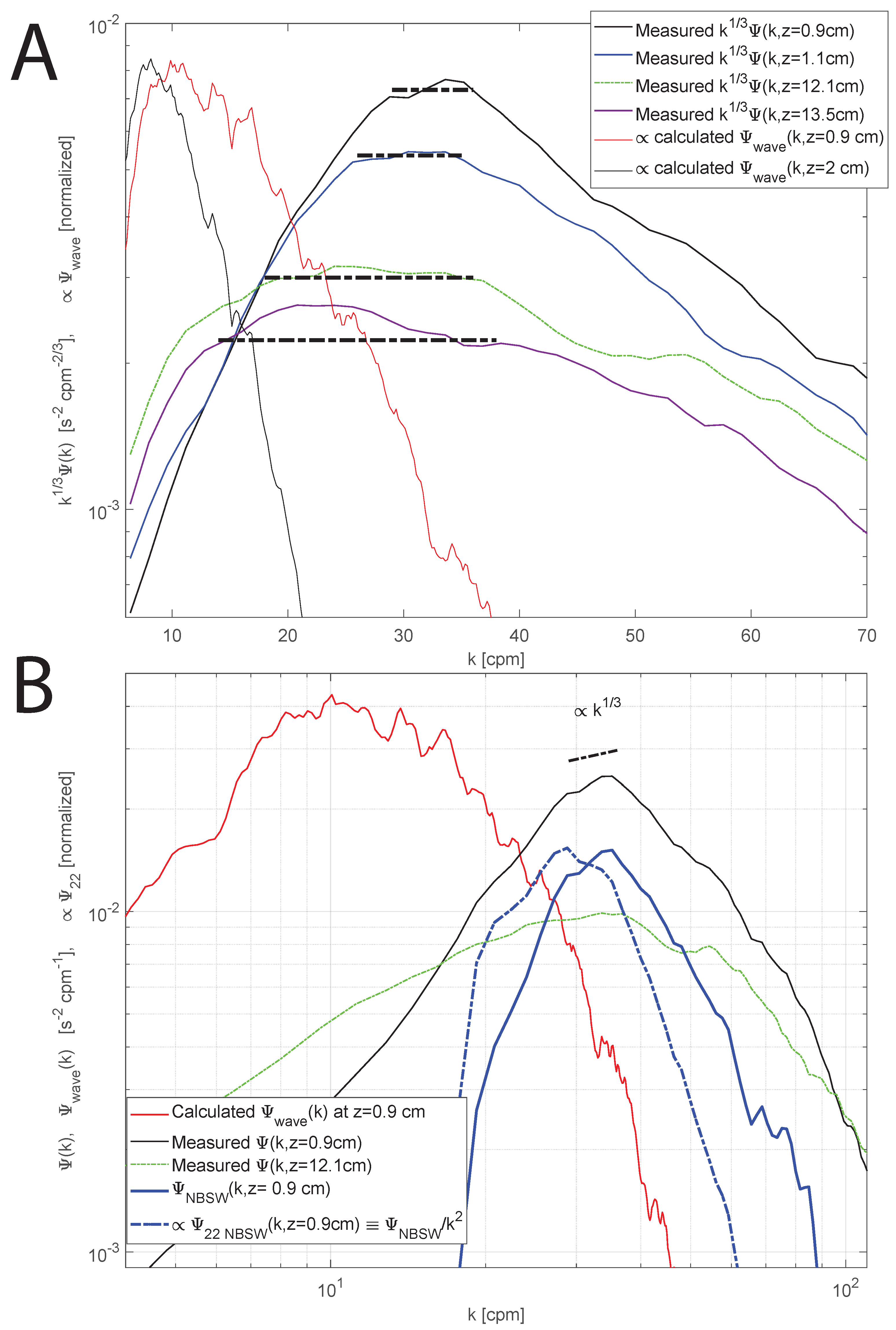
For the run with the current speed $U_{curr}=0.125$ m/s (Figure 2A), for selected depths, such as $0.9<z<13.5$ cm, we presented the measured compensated shear spectra, $k^{1/3}\Psi (k,z)$. The results were similar for the $U_{curr}=0.101$ and $U_{curr}=0.167$ m/s cases. Note that in following discussion, the calculated wave shear and the measured shear spectra are denoted as ${\Psi }_{wave}(k,z)$ and $\Psi (k,z)$, respectively. The flat part of the $k^{1/3}\Psi (k,z)$ spectrum, marked by dashed lines, corresponds to the extent of the inertial subrange. Note that for depths z larger than the dominant wavelength, $z>\lambda =8$ cm, the NBSW contribution to the background shear should be vanishing, as the background shear decreases exponentially with the depth, z, following Equation (10). That was reflected by the approximately similar extent of the inertial part spectrum for depths $z>8$ cm. We thus assume that at depths $z>8$ cm, the $\Psi (k,z)$ represents the spectra of the background turbulent flow. That background turbulent flow was characterized by a large microscale $R{e}_{\lambda }>487$, resulting in a well-developed turbulent background flow [16]. Initially, at depth $z>8$ cm, a very broad extent of the inertial subrange of the background turbulent flow, spanning wavenumbers 15–35 cpm (Figure 2A), became relatively narrow closer to the surface, and only $\approx 5$ cpm wide at the depth of $z=0.9$ cm. At that depth and well within the wave-affected depth, the decrease of the inertial range extent coincided with the increase of the $\Psi \left(k\right)$ level (Figure 2A). That transformation of the $k^{1/3}\Psi \left(k\right)$ spectra with depth was consistent with the transition from the background turbulent flow to the NBSW-dominated near-surface turbulent flow (Figure 2A).

The nature of the interaction between surface waves and the background flow can be studied by analyzing the relation between the range of wavenumbers where irrotational surface waves inject energy to the background turbulent flow and the location of the inertial range onset within the observed turbulent flow. At any given depth, the surface wave injects energy to the turbulent flow at the wavenumbers centered around the spectral peak of the surface wave shear, ${\Psi }_{wave}$ (see Equations (1) and (9)). In turn, the inception of the inertial subrange of the observed shear spectrum indicates the end of the wavenumber range where energy is injected into the turbulent flow. At the $z=0.9$ cm depth, the irrotational wave shear spectrum, ${\Psi }_{wave}(k,z=0.9\mathrm{cm})$, had a peak at 10 cpm. That peak was well separated from the inception of the inertial subrange of the $k^{1/3}\Psi (k,z=0.9\mathrm{cm})$, located at around 30 cpm. Note the strong depth dependence of the ${\Psi }_{wave}(k,z)$ spectrum peak and its width with depth. At the depth of 2 cm, the spectral peak of the ${\Psi }_{wave}(k,z=2\mathrm{cm})$ was shifted to larger-length scales while becoming narrower (Figure 2A).

The background shear spectrum was assumed to be well approximated by the measured shear at the depth $12.1$ cm, $\Psi (k,z=12.1\mathrm{cm})$ (the subsequent analysis would not quantitatively be changed if we had selected $\Psi (k,z=13.5\mathrm{cm})$). We further have assumed that in the absence of the surface waves, the grid-generated background turbulence was variable with the horizontal distance to the grid, but uniform in the vertical direction with the exception of a few millimeters-thick near-surface boundary [30]. Away from the thin surface boundary, we have approximated the NBSW-generated, depth-dependent shear spectrum, ${\Psi }_{NBSW}(k,z)$, by subtracting background shear from shear measured at that depth, i.e., ${\Psi }_{NBSW}(k,z=0.9\mathrm{cm})\approx \Psi (k,z=0.9\mathrm{cm})-\Psi (k,z=12.1\mathrm{cm})$. The ${\Psi }_{NBSW}$ spectra were principally used here to infer and illustrate the extent of wavenumbers affected by the action of the irrotational waves shear ${\Psi }_{wave}(k,z)$. On other hand, the quantity ${ϵ}_{NBSW}\left(z\right)\equiv \frac{15}{2}\nu {\int }_0^{\infty }\Psi (k,z=0.9\mathrm{cm})dk-\frac{15}{2}\nu {\int }_0^{\infty }\Psi (k,z=12.1\mathrm{cm})dk$ has a perfectly well-defined physical meaning as it represents a difference in the amount of irreversible viscous dissipation between two turbulent fluid flows: the background turbulent flow without NBSW and the fluid where the NBSW has interacted with background turbulent flow. Furthermore, we posit that the ${\Psi }_{NBSW}(k,z=0.9\mathrm{cm})$ spectrum, as defined above, may be used to approximate the NBSW shear spectra if the turbulent energy transfer is localized. For example, for turbulent flows, the numerical simulations and theoretical considerations [31] suggest that at a large Reynolds number (such as our background flow) the dominant non-local energy transfer is from the large to the small flow scales. Since the resultant NBSW turbulence was characterized by a short inertial range (not much energy contained in the large scales), as observed in reference [11], the resultant NBSW turbulence energy transfer is likely localized. We plan on investigating the NBSW-associated turbulent energy transfer details in follow-up research.

The ${\Psi }_{NBSW}(k,z=0.9\mathrm{cm})$ is presented in Figure 2B. The ${\Psi }_{NBSW}(k,z=0.9\mathrm{cm})$ shear spectrum had a very short inertial subrange bounded by wavenumbers 30–36 cpm. The NBSW one-dimensional velocity spectrum, defined as ${\Psi }_{22NBSW}(k,z=0.9\mathrm{cm})\equiv {\Psi }_{NBSW}(k,z=0.9\mathrm{cm})/k^2$, exhibits a peak at the beginning of its inertial subrange, at $k_{NBSW}=30$ cpm. That wavenumber, $k_{NBSW}$, corresponds to the length scale, where the NBSW injected energy into the existing turbulent flow. We posit that at the depth $z=0.9$ cm, the velocity spectrum ${\Psi }_{22NBSW}$ level increase above the background level, was due to action of the irrotational large-scale ($4<k<11$ cpm) NBSW shear, ${\Psi }_{wave}(k,z=0.9\mathrm{cm})$ on the background turbulent shear, taken as $\Psi (k,z=12.1\mathrm{cm})$ (Figure 2B).

Based on Figure 2A,B, within the depths comparable to the NBSW wavelength, we posit the following hypothesis of the NBSW turbulent dissipation: the energetic large-scale components of irrotational wave shear flow laminarized (or decreased the variance of) the largest scales of the turbulent background flow up to wavenumber $k_{NBSW}$. In turn, at that wavelength, the NBSW has injected energy into the background turbulent flow, thus increasing the level of the ${\Psi }_{NBSW}(k,z)$. That process resulted in elevated NBSW wave dissipation when compared to the background TKED. The effect of that process seems to be more pronounced as we approach the surface, as demonstrated by shortening the ${\Psi }_{NBSW}(k,z)$ inertial subrange length. That hypothesis is well supported by shadowgraph-like observations of the NBSW waves in reference [11]. The authors in reference [11] have documented, just before the wave peak arrival, the existence of initially large-length-scale laminar streaks followed by the appearance of small-scale and large-gradient features, right after the wave peak passage. That observation is consistent with NBSW laminarizing large scales up to a $k_{NBSW}$-length scale and then injecting velocity variance at wavenumbers above the wavenumber $k_{NBSW}$. In physical space, that process would result in the creation of small-scale, large-gradient structures.

Figure 2A,B, documented the presence of a well-delineated spectral gap between wave-induced irrotational shear flow and the NBSW-induced background turbulent flow, ${\Psi }_{NBSW}\left(k\right)$ and $\Psi \left(k\right)$. That observation supports the application of the Reynolds averaging approach parameterizing the NBSW turbulence, as taken by Teixeira and Belcher [12] or reference [11], and is consistent with our attempt here to parameterize the turbulent effects of the NBSW in the terms of the ratio $(T/{\tau }_{\eta })$. Following earlier arguments, we partitioned the observed TKED ${ϵ}_T\left(z\right)$ as: ${ϵ}_T\left(z\right)={ϵ}_{back}+{ϵ}_{NBSW}\left(z\right)$, a sum of grid-generated, depth-independent background TKED, ${ϵ}_{back}$, and the depth-dependent NBSW TKED contribution, ${ϵ}_{NBSW}\left(z\right)$, given by Equation (8). Note that a split into a bulk and the boundary energy dissipation has been frequently used to describe turbulent flows [32,33].

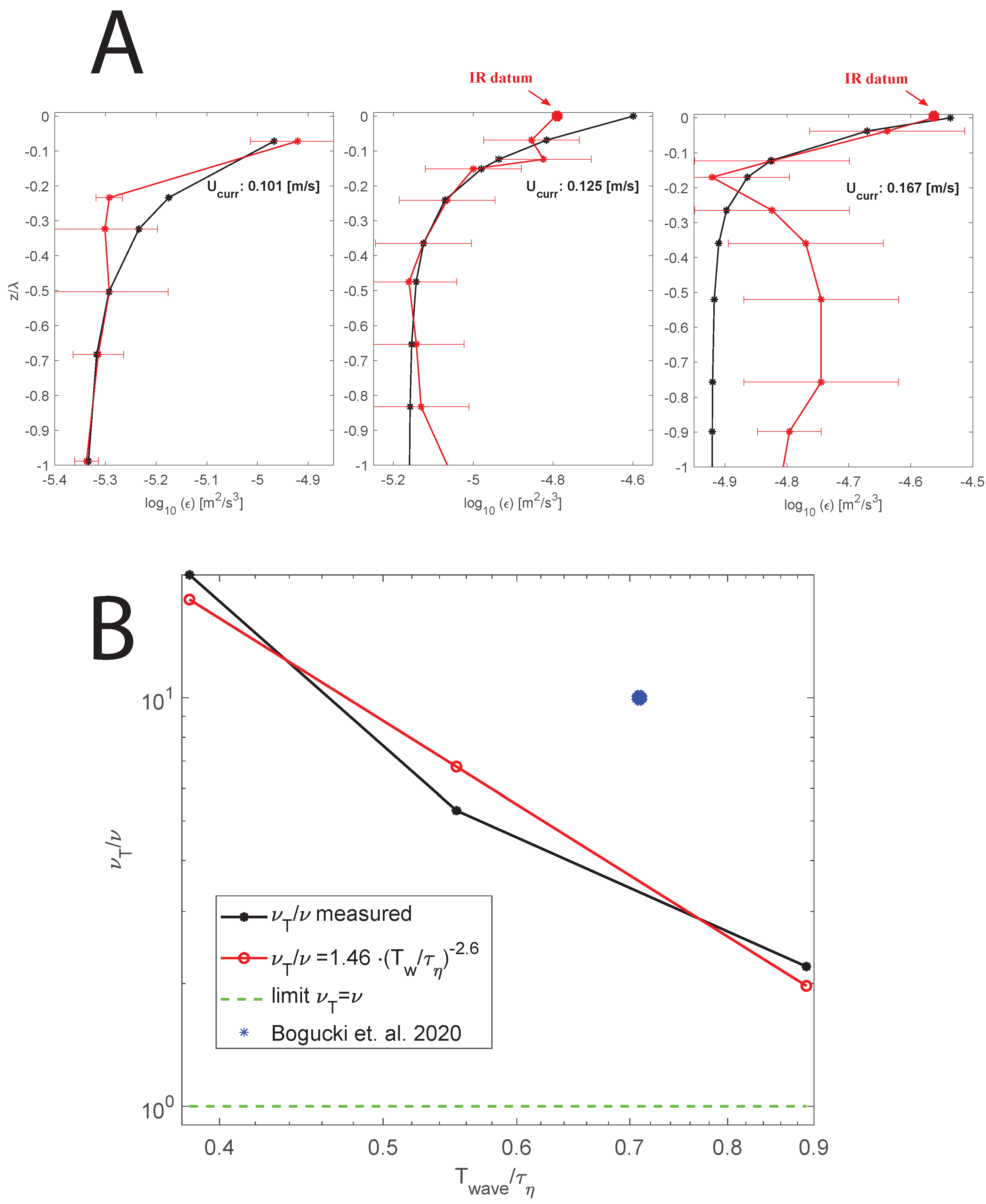
In each experiment, we varied the mean current speed, $U_{curr}$, as $0.1<U_{curr}<0.17$ m/s. The effect of the current speed increase was to elevate the background TKED (Figure 2B), as observed in reference [34]. In each run, the depth-independent background TKED, ${ϵ}_{back}$, was chosen to be the lowest TKED observed in the profile, typically at depths of around $z=15$ cm, and thus was largely unaffected by the NBSW (Equation (8)). The partitioned vertical profiles of the ${ϵ}_T\left(z\right)$ and the ${ϵ}_{NBSW}\left(z\right)$ as a function of the depth normalized by the dominant wavelength are presented in Figure 3A. The ${\nu }_T$ was obtained as a fit of ${ϵ}_{NBSW}\left(z\right)$ given by the Equation (8) to measured data (Figure 3A).

In each profile, the procedure to obtain ${\nu }_T$ from measured $ϵ\left(z\right)$ was as follows: (1) find the lowest value of the measured $ϵ\left(z\right)$, typically at 20 cm depth, and assign that value to ${ϵ}_{back}$; (2) find the best value of the ${\nu }_T$, by least square fitting ${ϵ}_{NBSW}\left(z\right)$, Equation (8), to $ϵ\left(z\right)-{ϵ}_{back}$ such that ${ϵ}_{NBSW}\left(z\right)\approx ϵ\left(z\right)-{ϵ}_{back}$.

Note that the corresponding IR-measured surface TKED values (Figure 3A) were somewhat smaller than predicted by the relationship Equation (8) when calculated for $z=0$. We attribute differences to a thin strongly rotational near-surface boundary, which tends to efficiently diffuse and homogenize the near-surface TKED values [14]. In the run $U_{curr}=0.167$ m/s and later, we noted the emergence of cross-stream wavefield components. The effect of cross-stream long waves (Equation (8)), was to elevate the TKED over a larger depth range than the along-tank waves. The near-surface TKED remained dominated by the along-tank waves. As a result, for the $U_{curr}=0.167$ m/s run (Figure 3A), only three TKED values closest to the surface TKED matched (including IR) predicted TKED values, Equation (8).

The NBSW eddy viscosity, ${\nu }_T$ (Equation (1)), observed in our runs, was best explained when expressed as ${\nu }_T^{*}\equiv {\nu }_T/\nu =1.46{(T/{\tau }_{\eta })}^{-2.6}$ (Figure 3B), where ${\tau }_{\eta }$ is the Kolmogorov time scale ${\tau }_{\eta }={(\nu /ϵ)}^{1/2}$ with the $ϵ$ of the background flow. Values of ${\nu }_T^{*}$ are somewhat smaller than in reference [11], where they observed ${\nu }_T/\nu =10$ but they did not record the $ϵ$ of the background flow.

To assess the sensitivity of our results (Figure 3A,B) to the assumptions leading to the derivation of the Equation (7), we have carried out calculations with the wave attenuation factor switched off, i.e., we set $H(f,L)\equiv 1$. Our results and conclusions remained qualitatively the same, while the estimated ${\nu }_T^{*}$ range became $1<{\nu }_T^{*}<4.2$ instead of $1<{\nu }_T^{*}<20$, as presented here.

4. Discussion

At the first glance, our results presented in Figure 3B appear to be counter-intuitive, as they suggest that the non-breaking waves tend to lose energy slower in the more turbulent background flow, since $T/{\tau }_{\eta }\propto {ϵ}^{1/2}$, resulting in ${\nu }_T^{*}\propto {ϵ}^{-1.3}$. We suspect that this observation is an artifact of a small range of investigated ratios $T/{\tau }_{\eta }\le 0.9$. For oceanic swell with $T=10$ s and the ${ϵ}_{back}=5\times {10}^{-6}$ W/kg, we expect the ratio $T/{\tau }_{\eta }>20$.

The direct shear measurements have demonstrated the presence of a spectral gap between NBSW-generated shear and the spectral peak of the background turbulent shear. The interpretation of our shear measurements was consistent with the hypothesis of the NBSW turbulence-generating mechanism, where the wave irrotational shear tends to depress large-scale flow variance while transferring energy to shorter-length scales. That resulted in a shortening of the inertial subrange and increased the TKED of the NBSW-generated turbulent flow.

Based on our experiment, we can not fully assess the universality of our results, owing to the small observed $T/{\tau }_{\eta }$ range; however, consistently with the hypothesis, we expect the oceanic NBSW near-surface turbulence to be characterized by a short inertial range or the elevated TKED, as observed here or in reference [11].

5. Conclusions

Surface waves play an important role in the exchange of mass, momentum, and energy between the atmosphere and the ocean. Our work presented here addresses a significant knowledge gap in understanding turbulent processes associated with the non-breaking oceanic waves, a defining oceanic feature covering over 90% of the ocean surface. Until recently, the existence of non-breaking wave-induced turbulence had been given little attention, although its presence has been suggested by observations. The knowledge gap in the understanding of the NBSW contribution to the oceanic turbulence resulted in poorly understood physics of the oceanic heat or the $C{O}_2$ exchange processes at low wind speeds.

Our observations when $(T/{\tau }_{\eta })<0.9$ have demonstrated that the eddy viscosity associated with the NBSW was consistent with ${\nu }_T/\nu =1.46{(T/{\tau }_{\eta })}^{-2.6}$. The existence of a spectral gap between irrotational wave shear and the background of the NBSW-generated shear dissipation spectrum suggests that the NBSW turbulent dissipation can be explored in terms of the Reynolds averaging of the Navier–Stokes turbulence models, such as, for example, the approaches in reference [12] or reference [11].

Our measurement results are limited by the fact that the investigated parameter space was restricted to $(T/{\tau }_{\eta })<0.9$. Based on our measurements, and within the investigated parameter space, it appears that the background turbulence within the measurement ranges acted as a ‘wave lubricant’. Our results represent the first attempt to quantify NBSW dissipation in terms of the strength of preexisting background turbulence and more work is needed to expand our results to a oceanic-relevant $(T/{\tau }_{\eta })$ parameter space.

References

- Terray, E.A.; Donelan, M.; Agrawal, Y.; Drennan, W.M.; Kahma, K.; Williams, A.J.; Hwang, P.; Kitaigorodskii, S. Estimates of kinetic energy dissipation under breaking waves. J. Phys. Oceanogr. 1996, 26, 792–807. [Google Scholar] [CrossRef] [Green Version]
- Craig, P.D.; Banner, M.L. Modeling wave-enhanced turbulence in the ocean surface layer. J. Phys. Oceanogr. 1994, 24, 2546–2559. [Google Scholar] [CrossRef] [Green Version]
- Ferrari, R.; Wunsch, C. Ocean circulation kinetic energy: Reservoirs, sources, and sinks. Annu. Rev. Fluid Mech. 2009, 41, 253–282. [Google Scholar] [CrossRef] [Green Version]
- Huang, C.J.; Qiao, F.; Song, Z.; Ezer, T. Improving simulations of the upper ocean by inclusion of surface waves in the Mellor-Yamada turbulence scheme. J. Geophys. Res. Ocean. 2011, 116, C01007. [Google Scholar] [CrossRef] [Green Version]
- Zhuang, Z.; Zheng, Q.; Yuan, Y.; Yang, G.; Zhao, X. A non-breaking-wave-generated turbulence mixing scheme for a global ocean general circulation model. Ocean Dyn. 2020, 70, 293–305. [Google Scholar] [CrossRef]
- Phillips, O. On the dynamics of unsteady gravity waves of finite amplitude Part 2. Local properties of a random wave field. J. Fluid Mech. 1961, 11, 143–155. [Google Scholar] [CrossRef]
- Gemmrich, J.R.; Banner, M.L.; Garrett, C. Spectrally resolved energy dissipation rate and momentum flux of breaking waves. J. Phys. Oceanogr. 2008, 38, 1296–1312. [Google Scholar] [CrossRef]
- Thais, L.; Magnaudet, J. Turbulent structure beneath surface gravity waves sheared by the wind. J. Fluid Mech. 1996, 328, 313–344. [Google Scholar] [CrossRef]
- Gargett, A.; Osborn, T.; Nasmyth, P. Local isotropy and the decay of turbulence in a stratified fluid. J. Fluid Mech. 1984, 144, 231–280. [Google Scholar] [CrossRef]
- Anguelova, M.D.; Webster, F. Whitecap coverage from satellite measurements: A first step toward modeling the variability of oceanic whitecaps. J. Geophys. Res. Ocean. 2006, 111, C03017. [Google Scholar] [CrossRef] [Green Version]
- Bogucki, D.J.; Haus, B.K.; Barzegar, M.; Shao, M.; Domaradzki, J.A. On the Nature of the Turbulent Energy Dissipation Beneath Nonbreaking Waves. Geophys. Res. Lett. 2020, 47, e2020GL090138. [Google Scholar] [CrossRef]
- Teixeira, M.; Belcher, S. On the distortion of turbulence by a progressive surface wave. J. Fluid Mech. 2002, 458, 229–267. [Google Scholar] [CrossRef]
- Ardhuin, F.; Jenkins, A.D. On the interaction of surface waves and upper ocean turbulence. J. Phys. Oceanogr. 2006, 36, 551–557. [Google Scholar] [CrossRef]
- Landau, L.; Lifshitz, E. Vol 6: Fluid Mechanics; Addison-Wesley Mass: Boston, MA, USA, 1959. [Google Scholar]
- Harkins, W.D.; Brown, F. The determination of surface tension (free surface energy), and the weight of falling drops: The surface tension of water and benzene by the capillary height method. J. Am. Chem. Soc. 1919, 41, 499–524. [Google Scholar] [CrossRef]
- Zhou, T.; Antonia, R. Reynolds number dependence of the small-scale structure of grid turbulence. J. Fluid Mech. 2000, 406, 81–107. [Google Scholar] [CrossRef]
- De Padova, D.; Mossa, M.; Sibilla, S. SPH modelling of hydraulic jump oscillations at an abrupt drop. Water 2017, 9, 790. [Google Scholar] [CrossRef] [Green Version]
- Donelan, M.A.; Haus, B.K.; Plant, W.J.; Troianowski, O. Modulation of short wind waves by long waves. J. Geophys. Res. Ocean. 2010, 115, C10003. [Google Scholar] [CrossRef] [Green Version]
- Massel, S.R. On the geometry of ocean surface waves. Oceanologia 2011, 53, 521–548. [Google Scholar] [CrossRef] [Green Version]
- Macoun, P.; Lueck, R. Modeling the spatial response of the airfoil shear probe using different sized probes. J. Atmos. Ocean. Technol. 2004, 21, 284–297. [Google Scholar] [CrossRef]
- Klettner, C.A.; Eames, I. The laminar free surface boundary layer of a solitary wave. J. Fluid Mech. 2012, 696, 423–433. [Google Scholar] [CrossRef]
- Lueck, R. RSI Technical Note 030: On the Forms of the Velocity, Shear, and Rate-of-Strain Spectra; Rockland Scientific International: Victoria, BC, Canada, 2014; Available online: http://rocklandscientific.com/support/knowledge-base/technical-notes (accessed on 24 May 2022).
- Oakey, N.S. Determination of the rate of dissipation of turbulent energy from simultaneous temperature and velocity shear microstructure measurements. J. Phys. Oceanogr. 1982, 12, 256–271. [Google Scholar] [CrossRef] [Green Version]
- Lumley, J.; Terray, E. Kinematics of turbulence convected by a random wave field. J. Phys. Oceanogr. 1983, 13, 2000–2007. [Google Scholar] [CrossRef] [Green Version]
- Moum, J.N. Energy-containing scales of turbulence in the ocean thermocline. J. Geophys. Res. Ocean. 1996, 101, 14095–14109. [Google Scholar] [CrossRef]
- Metoyer, S.; Barzegar, M.; Bogucki, D.; Haus, B.K.; Shao, M. Measurement of small-scale surface velocity and turbulent kinetic energy dissipation rates using infrared imaging. J. Atmos. Ocean. Technol. 2020, 38, 269–282. [Google Scholar] [CrossRef]
- Collins, C.O., III; Blomquist, B.; Persson, O.; Lund, B.; Rogers, W.; Thomson, J.; Wang, D.; Smith, M.; Doble, M.; Wadhams, P. Doppler correction of wave frequency spectra measured by underway vessels. J. Atmos. Ocean. Technol. 2017, 34, 429–436. [Google Scholar] [CrossRef] [Green Version]
- Zhang, X. Enhanced dissipation of short gravity and gravity capillary waves due to parasitic capillaries. Phys. Fluids 2002, 14, L81–L84. [Google Scholar] [CrossRef]
- Bluteau, C.E.; Jones, N.L.; Ivey, G.N. Estimating turbulent dissipation from microstructure shear measurements using maximum likelihood spectral fitting over the inertial and viscous subranges. J. Atmos. Ocean. Technol. 2016, 33, 713–722. [Google Scholar] [CrossRef]
- Murzyn, F.; Bélorgey, M. Experimental investigation of the grid-generated turbulence features in a free surface flow. Exp. Therm. Fluid Sci. 2005, 29, 925–935. [Google Scholar] [CrossRef]
- Domaradzki, J.; Rogallo, R. Local energy transfer and nonlocal interactions in homogeneous, isotropic turbulence. Phys. Fluids A 1990, 2, 413. [Google Scholar] [CrossRef]
- Ahlers, G.; Grossmann, S.; Lohse, D. Heat transfer and large scale dynamics in turbulent Rayleigh-Bénard convection. Rev. Mod. Phys. 2009, 81, 503–537. [Google Scholar] [CrossRef] [Green Version]
- Zhang, Y.; Zhou, Q.; Sun, C. Statistics of kinetic and thermal energy dissipation rates in two-dimensional turbulent Rayleigh–Bénard convection. J. Fluid Mech. 2017, 814, 165–184. [Google Scholar] [CrossRef]
- Roach, P.E. The generation of nearly isotropic turbulence by means of grids. Int. J. Heat Fluid Flow 1987, 8, 82–92. [Google Scholar] [CrossRef]
- DiCiccio, T.J.; Efron, B. Bootstrap confidence intervals. Stat. Sci. 1996, 11, 189–228. [Google Scholar] [CrossRef]
Figure 1.
(A) Schematic depiction of the experimental setup and the side view of instruments location: VMP200, current meter, IR camera, and details of the grid arrangement. (B) Example of observed wave properties for m/s. From the top: (I) Observed directional wave slope variance spectra aligned with the tank axis x. (II) Intrinsic directional wave variance spectra. Blueline, the spectra used for calculations. (III) Intrinsic wave variance spectra transformed to the VMP200 site. (C) The dominant wave, i.e., the wave with the largest slope, and its properties: wave slope, wavelength, phase speed, and current speed generated by the wave 1 cm below the surface for , , and m/s. Bottom-the background TKED dissipation.
Figure 2.
(A) Measured compensated shear spectra, for the case m/s characterized by the NBSW with a dominant wave length of 8 cm. The shear spectra are compared to normalized , obtained from the Equation (10) at depths and 2 cm and at the location. The horizontal dashed lines represent approximate extent of the inertial subrange. (B) Black line: the measured shear spectrum at depth z = 0.9 cm compared with calculated —corresponding to the red line. The continuous blue line: the . The blue dashed line: the velocity spectrum: . The black dashed line: the approximate extent of the inertial subrange of the spectrum. Note the peak in the at the beginning of its inertial subrange at around the wavenumber kNBSW = 30 cpm.
Figure 3.
(A) Partitioned vertical TKED profiles for different current speeds : red—the observed TKED ; black—the sum of the derived from Equation (8); and the —a depth-independent background TKED. The error bar corresponds to the estimated 95% confidence interval [35] of the measured TKED. The depth is normalized by the dominant wavelength in each run (Figure 1C). (B) The derived as a function of the wave period T to the Kolmogorov microscale time . Fit to experimental data yielded: . The blue dot—the result from NBSW measurements reported in Bogucki et al. [11].
Publisher’s Note: MDPI stays neutral with regard to jurisdictional claims in published maps and institutional affiliations. |
© 2022 by the authors. Licensee MDPI, Basel, Switzerland. This article is an open access article distributed under the terms and conditions of the Creative Commons Attribution (CC BY) license (https://creativecommons.org/licenses/by/4.0/).
Share and Cite
MDPI and ACS Style
Bogucki, D.J.; Haus, B.K.; Barzegar, M. Observations and Parametrization of the Turbulent Energy Dissipation Beneath Non-Breaking Waves. Fluids 2022, 7, 216. https://0-doi-org.brum.beds.ac.uk/10.3390/fluids7070216
AMA Style
Bogucki DJ, Haus BK, Barzegar M. Observations and Parametrization of the Turbulent Energy Dissipation Beneath Non-Breaking Waves. Fluids. 2022; 7(7):216. https://0-doi-org.brum.beds.ac.uk/10.3390/fluids7070216
Chicago/Turabian StyleBogucki, Darek J., Brian K. Haus, and Mohammad Barzegar. 2022. "Observations and Parametrization of the Turbulent Energy Dissipation Beneath Non-Breaking Waves" Fluids 7, no. 7: 216. https://0-doi-org.brum.beds.ac.uk/10.3390/fluids7070216