Deep Learning in LncRNAome: Contribution, Challenges, and Perspectives


1
College of Science and Engineering, Hamad Bin Khalifa University, Doha 34110, Qatar
2
School of Natural and Computational Sciences, Massey University, Auckland 0632, New Zealand
*
Author to whom correspondence should be addressed.
Non-Coding RNA 2020, 6(4), 47; https://0-doi-org.brum.beds.ac.uk/10.3390/ncrna6040047
Submission received: 25 July 2020
/
Revised: 27 October 2020
/
Accepted: 6 November 2020
/
Published: 30 November 2020
Abstract
:Long non-coding RNAs (lncRNA), the pervasively transcribed part of the mammalian genome, have played a significant role in changing our protein-centric view of genomes. The abundance of lncRNAs and their diverse roles across cell types have opened numerous avenues for the research community regarding lncRNAome. To discover and understand lncRNAome, many sophisticated computational techniques have been leveraged. Recently, deep learning (DL)-based modeling techniques have been successfully used in genomics due to their capacity to handle large amounts of data and produce relatively better results than traditional machine learning (ML) models. DL-based modeling techniques have now become a choice for many modeling tasks in the field of lncRNAome as well. In this review article, we summarized the contribution of DL-based methods in nine different lncRNAome research areas. We also outlined DL-based techniques leveraged in lncRNAome, highlighting the challenges computational scientists face while developing DL-based models for lncRNAome. To the best of our knowledge, this is the first review article that summarizes the role of DL-based techniques in multiple areas of lncRNAome.
1. Introduction
The transcriptional landscape in eukaryotic organisms (e.g., humans) is now perceived as far more intricate than was originally thought [1] after the discovery that only about 2% of the genomic regions in humans encode for proteins, and the remaining sequences are non-coding regions that do not encode for proteins [2]. Since most of the human genome is transcribed, whether it encodes a protein or not, a major part of the human genome is pervasively transcribed into non-coding RNAs (ncRNAs). From this expanded view of ncRNAs, long non-coding RNAs (lncRNAs), which are more than 200 nucleotides in length, have recently been in the limelight due to evidence of linking mutations in their sequence to the dysregulation in many human diseases [3]. For example, genome-wide association studies (GWAS) have discovered that the long non-coding RNA (lncRNA) ANRIL is significantly associated with susceptibility to type 2 diabetes, intracranial aneurysm, coronary disease, and several types of cancers [3]. There are several mutations within the ANRIL gene body, as well as in its surroundings, that are correlated with a propensity for developing the above-mentioned diseases [3]. Another example of an lncRNA is Gas5, which is involved in susceptibility to auto-immune disorders [4] and could also act as a tumor suppressor in breast cancer [5]. Besides these examples, numerous other lncRNAs are involved in a multitude of human diseases. Interested readers may refer to the following articles to get a more detailed picture of the role of lncRNAs in different diseases [3,6,7,8].
In the early 1980s, scientists used to consider the hybridization of complementary DNA (cDNA) for cloning the genes and measuring their expression and tissue-specificity [9]. Initially, the efforts were focused on genes that were known to produce proteins. Then, the scientific community adopted the same approach for RNAs without considering their coding potential. Based on this approach, the first discovered lncRNA in a eukaryotic organism was H19. The intriguing factor about the discovery of H19 was the absence of being translated even though it had small open reading frame sequences in the gene body. Surprisingly, the transcripts of H19 showed similar characteristics to those of messenger RNAs (mRNA) in terms of splicing, polyadenylation, localization in the cytoplasm, and its transcription by RNA polymerase II [10]. From the roster of the earliest discovered lncRNAs, X-inactive-specific transcript (XIST) is among the most well-studied lncRNAs due to its role in the X-chromosome inactivation (XCI) phenomena [11]. The loci of XIST was discovered in the early 1990s, and it showed very low expression levels in mouse undifferentiated embryonic stem (ES) cells for both males and females [12,13]. Since the pioneering discoveries of H19 and XIST, the view on non-coding genes in the scientific community has changed completely and has rejuvenated the efforts to discover and characterize novel non-coding RNAs. Specifically, studying lncRNAs has increased dramatically. Additionally, advancement in next-generation-sequencing technology enabled the discovery of many functional lncRNAs in the non-coding regions of the human genome. LncRNAs, despite being considered to be junk DNA regions for approximately the last twenty years [14], are now recognized as being pervasively transcribed, and non-coding RNA transcriptomes (specifically lncRNAs) have become a major field in biomedical research.
The pervasive nature of the transcriptomes in humans [15] and mice [16] has also been highlighted by the Functional Annotation of the Mammalian Genome (FANTOM) consortium in the largest collection of functional lncRNAs, with over 23,000 lncRNA genes [17]. GENCODE [18] v25 provides a list of ~18,000 human lncRNA genes. MiTranscriptome has collected 58,548 lncRNA genes [19], however, it is unclear if all of them are functional. From this, we can observe that the discovery of novel lncRNAs is becoming a regular occurrence, and the catalogue of lncRNAs is constantly growing. Therefore, it is of interest to analyze this large, versatile, and dynamic collection of lncRNAs in a systematic fashion using state-of-the-art computational techniques to derive novel hypotheses, discover unanticipated links, and make proper functional inferences [20]. Machine learning (ML)-based methods are well suited for lncRNA research, since ML-based techniques can generate insights and discover new patterns from the growing number of lncRNA repositories.
Though ML-based methods are applicable to different types of data, the performance of ML-based models depends on the representation of the data. The quality of data representation and the relevance of the data to a particular problem affect the performance of ML-based models. Deep learning (DL), a sub-field of ML, can address this issue by embedding the data for the model to yield end-to-end models [21]. DL, a biology-inspired neural network [22], uses multiple hidden layers and is considered to be among the best paradigms for classification and prediction in the ML field [23]. In the past ten years, DL-based models have achieved tremendous success in computer vision [24], machine translation [25], and speech recognition [26]. The main reason for their success is the unprecedented availability of massive volumes of data, improvement of computational capacity, and the advancement of sophisticated algorithms [27,28]. The enormous amount of biological data, which was once considered to be a big analysis challenge, transformed into an opportunity for biomedical researchers [29]. DL-based methods have now been successfully applied in the genomics research domain [21].
Considering the functionally diverse role of lncRNA in different human biological processes and diseases and the extreme capacity of DL to identify informative patterns from big data, we reviewed how DL has facilitated the discovery of the role of lncRNAs in different human diseases and the underlying mechanism in a data-driven fashion. To the best of our knowledge, this article is the first to summarize the contribution of DL in multiple research domains of lncRNAome.
We organized this article in the following way. We first introduce a primer on DL techniques that were successfully applied in different lncRNAome-related problems. Then, we highlight the DL-based methods that have been successfully applied in several lncRNA-related research problems. We continue by discussing potential issues that might be encountered by researchers while implementing DL-based solutions for lncRNAome and possible resolutions. Finally, we conclude by discussing the perspectives of DL methods in lncRNAome research areas.
2. Summary of Deep Learning Techniques that Are Applied in lncRNAome-Related Research Problems
In this section, we provide a brief description of the deep learning (DL) models that have successfully been used in the modeling of lncRNAome-related research problems.
2.1. Neural Network
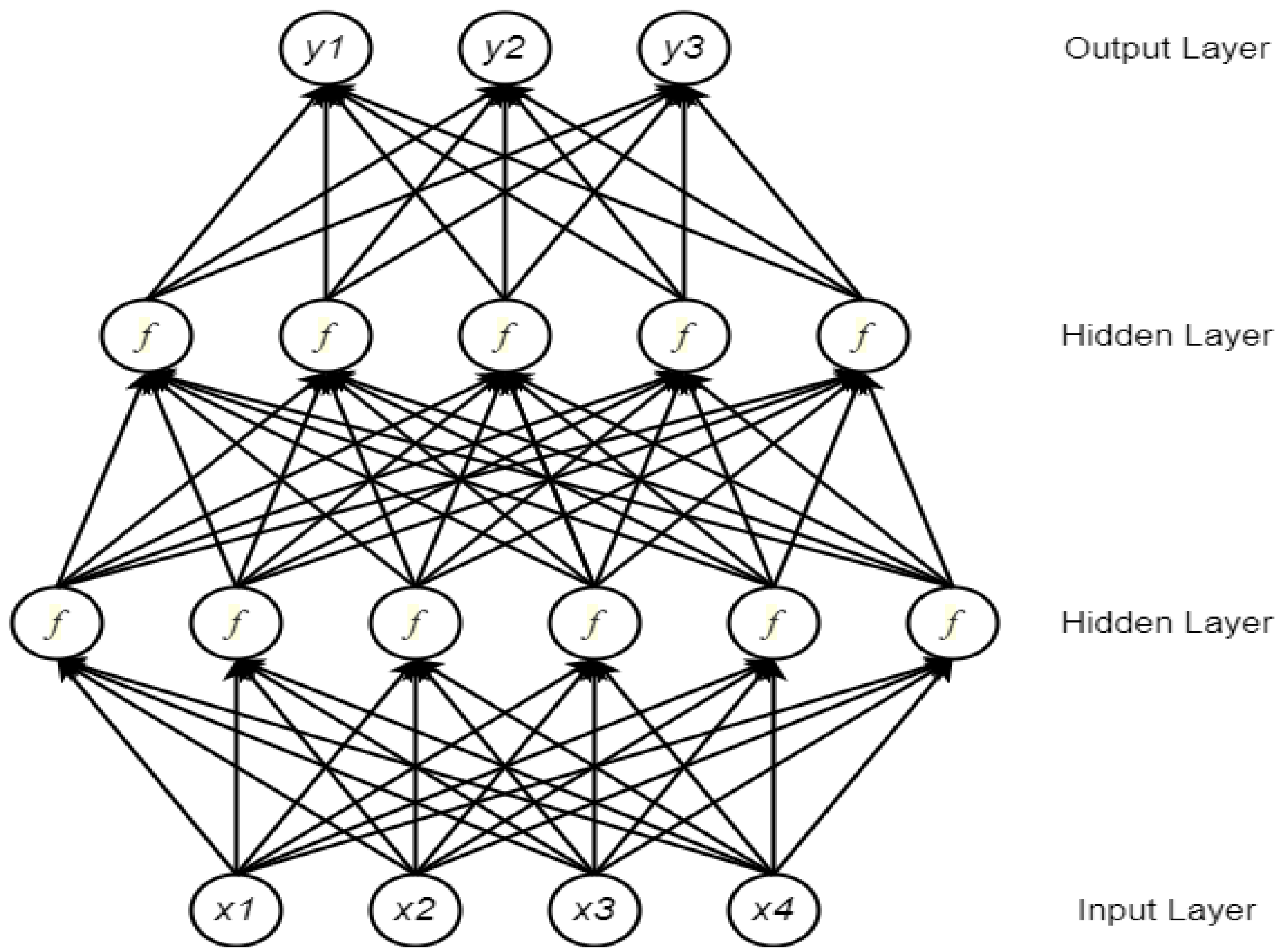
A neural network (NN) comprises multiple processing components, or parts, that are joined to form a network with adjustable weighting functions for each input. The NN components are organized in several connected layers. Typically, there are three types of layers in a NN: input layer, hidden layer(s), and output layer [30]. The input layer considers data to be fixed-size input values and presents them through the hidden layers inside the network. To propagate from one layer to the next, a weighted sum of the inputs from the previous layer is passed through a non-linear function. Finally, a fixed-sized output is generated through the output layer. Currently, the most popular function for the hidden layers is the rectified linear unit (ReLU) [31]. Depending on whether a task is a binary or a multi-class classification problem, a Sigmoid or a Softmax function is used at the output layer. Figure 1 shows a typical NN architecture for vector inputs.
2.2. Deep Neural Network
A deep neural network (DNN) is a neural network that has multiple hidden layers. These multiple learning layers allow for learning representations of data that have many levels of abstraction, which leads to improvements in model performance in many applications such as object detection, speech recognition, and many more [31].
2.3. Deep Belief Network
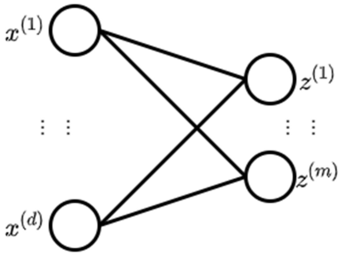
A deep belief network (DBN) is a network of multiple layers where each layer consists of a restricted Boltzmann machine (RBM) with a classifier in the last layer [33]. An RBM is a neural network with two layers where the left layer is the visible layer and the right layer is the hidden layer (Figure 2) [34]. The visible layer represents a less abstract form of the raw data where the hidden layer is trained to represent more abstract features [35].
2.4. Convolutional Neural Network
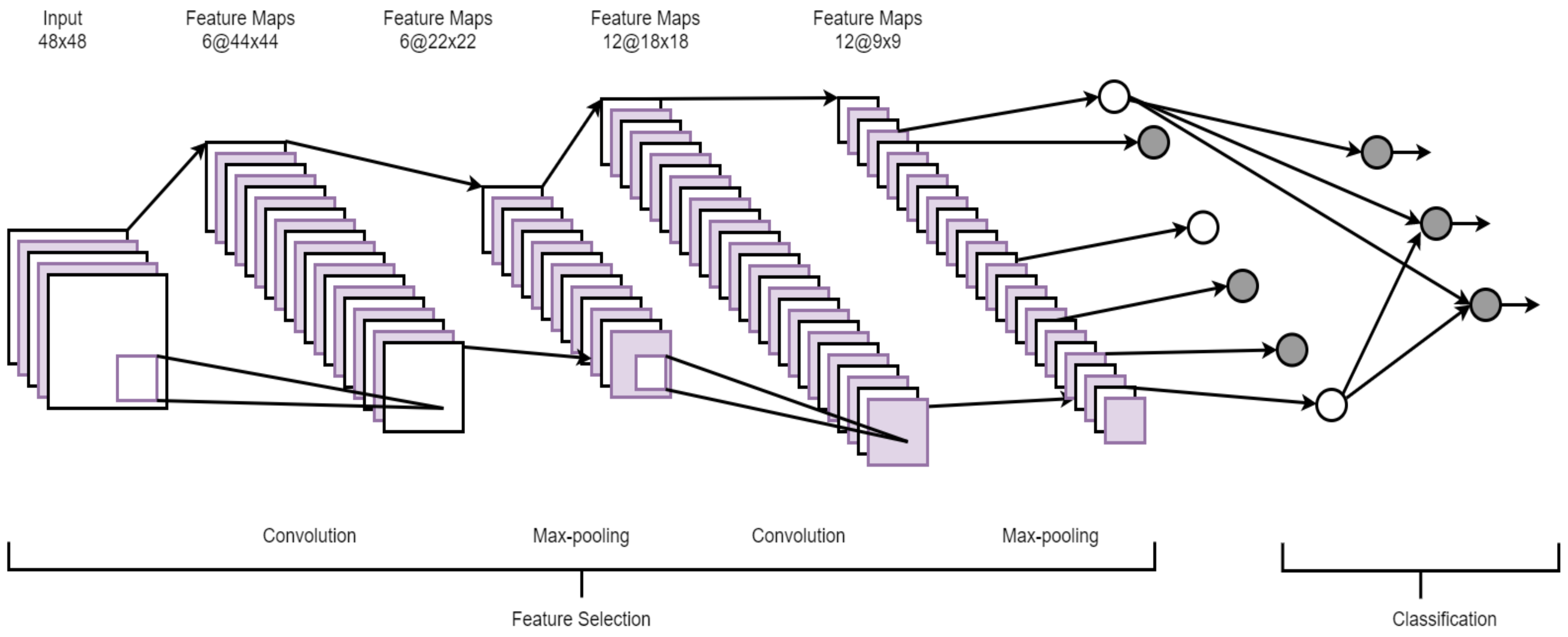
A convolutional neural network (CNN) is a hierarchical model that learns patterns at multiple layers using a series of 1D, 2D, or 3D convolutional operations [31]. A CNN usually consists of multiple layers, namely, a convolutional layer, a non-linearity layer, a pooling layer, and a fully-connected (FC) layer(s) [37]. However, it is important to stress that all of these layers are not mandatory to build a CNN. Multiple stages of these layers are followed by conventional fully connected layers. A set of filters is used in the convolutional layer to extract spatial features from the input data and the pooling layer reduces the dimension of the data after convolution steps. Since FC layers have a large number of parameters, making it harder to train the network, a new type of layer, global average pooling [38], can be applied directly to the output of the final convolution layer, eliminating the need for the FC. Since pooling operations might discard useful information from the input, strided convolution has recently been researchers’ preference. Figure 4 shows the architecture of a typical CNN.
2.5. Graph Convolutional Network
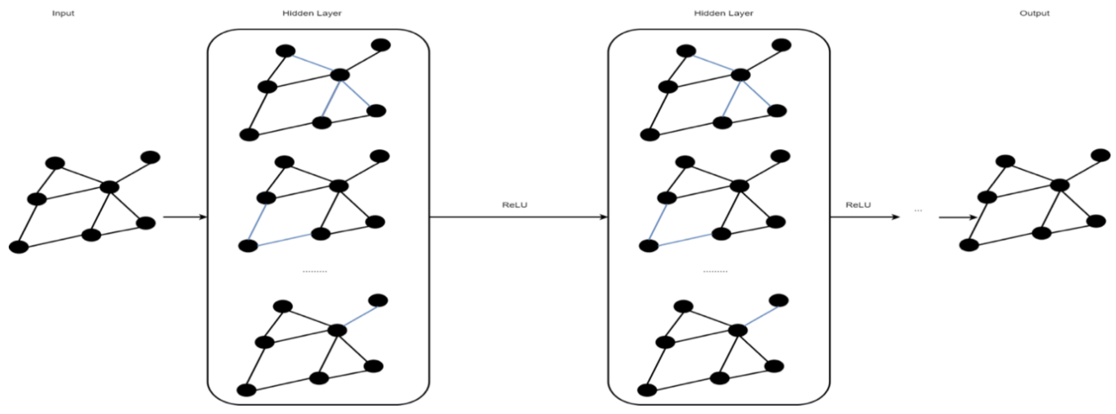
A graph convolutional network (GCN) is a type of convolutional neural network that works on graphs [40]. A GCN’s input is a graph with labeled nodes, and the output is all the input graph’s nodes labeled as predictions. Similar to CNNs or multi-layer perceptrons (MLP), for any input, a GCN learns new features that later become inputs to the classifier over multiple layers. Unlike an MLP, at the beginning of each layer, a GCN averages the features of each node with feature vectors in the neighborhood [40]. Figure 5 shows an example of a GCN.
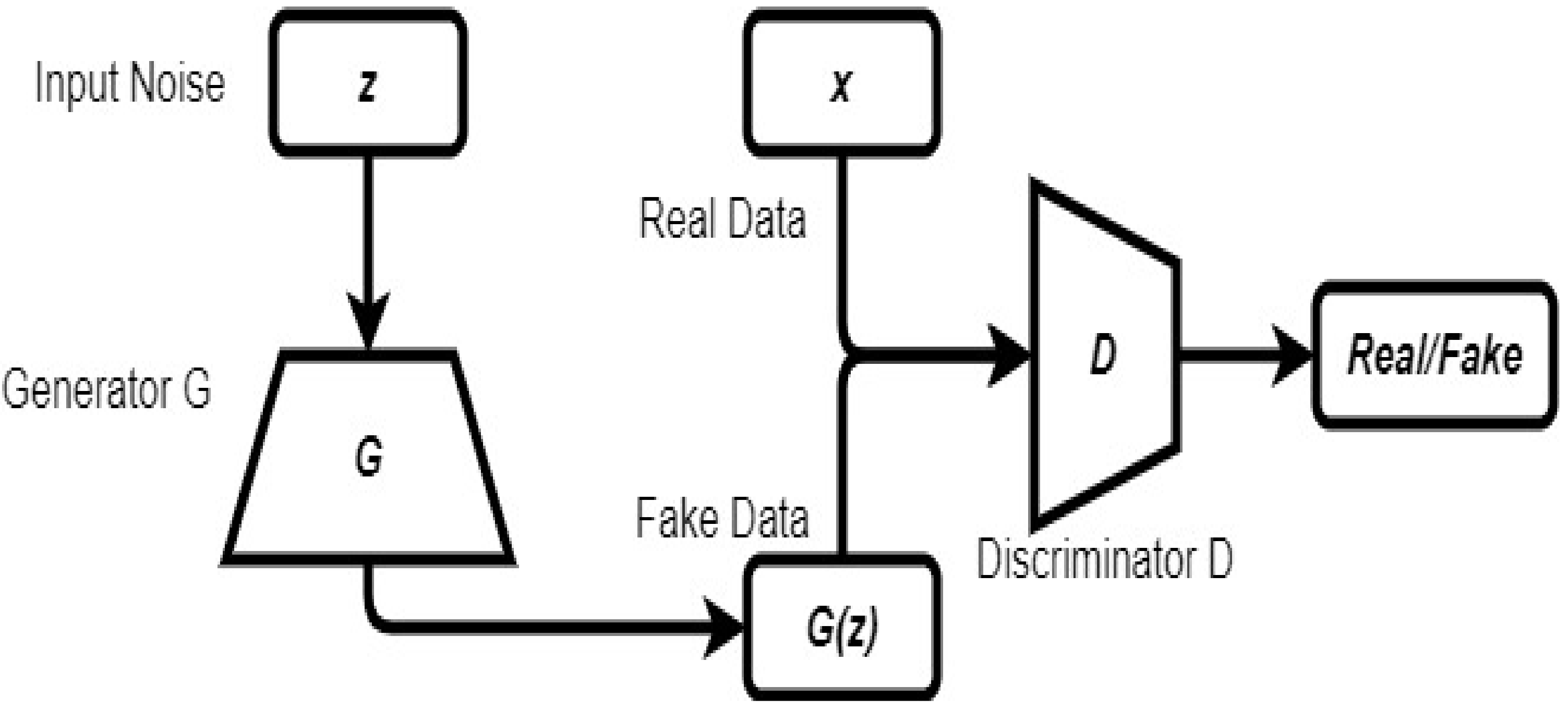
2.6. Generative Adversarial Network
A generative adversarial network (GAN) is a model that comprises generative and discriminative models. Both models are trained in an adversarial manner where the generator generates fake inputs that seem real, and the discriminative model tries to classify inputs as either real or fake [42]. In this model, the training process for the generator is to maximize the probability of the discriminator making a mistake [43]. This model can be used in applications related to data synthesis, classification, and image super-resolution [42]. Figure 6 shows an architecture of a GAN.
2.7. Autoencoder
An autoencoder (AE) is a type of neural network that learns the latent, lower-dimensional representation of input variables by passing the input variables through a bottleneck layer in the middle of the network and reconstructing the input variable at the output layer [44]. The loss function used in training this network penalizes the input reconstruction error. After convergence, the trained network can be used for input reconstruction with minimal noise [45]. One of the advantages of an AE is that it can be used in learning a lower-dimensional representation of input data with low reconstruction error even when it spans a non-linear manifold in a feature space. Figure 7 shows an architecture of an AE.
2.8. Recurrent Neural Network
A recurrent neural network (RNN) is made of artificial neurons with one or more feedback loops. A simple RNN architecture consists of an input layer, multiple recurrent hidden layer(s), and an output layer [46]. An RNN constructs recurrent connections over a period of time, and activation from time steps is stored in the internal memory of the network. This makes an RNN suitable for applications related to time series and sequential data [47]. Figure 8 shows an architecture of an RNN.
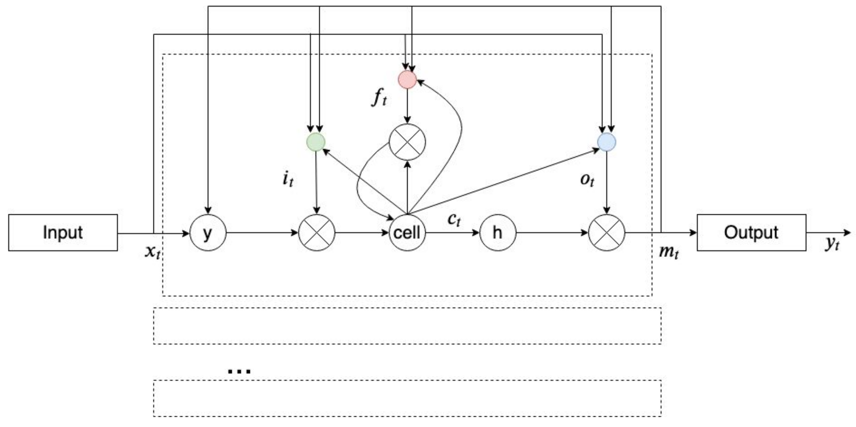
A long short-term memory (LSTM) is a type of RNN that reduces the effects of vanishing and exploding gradients (which is a drawback of an RNN that happens during the training of an RNN) in an RNN. LSTM changes the structure of hidden units from “sigmoid” or “tanh” to memory cells where gates control inputs and outputs and maintain extracted features from preceding timesteps [48]. Figure 9 shows an LTSM memory block.
A bidirectional LSTM (BLSTM) is a variation of an RNN [50] that runs in both forward and backward directions, where the output from a cell depends on all the previous (forward direction) and future (backward direction) timesteps. A BLSTM has been found to perform better than a unidirectional LSTM if the output at a timestep depends on both past and future inputs. Figure 10 shows a typical BLTSM network structure.
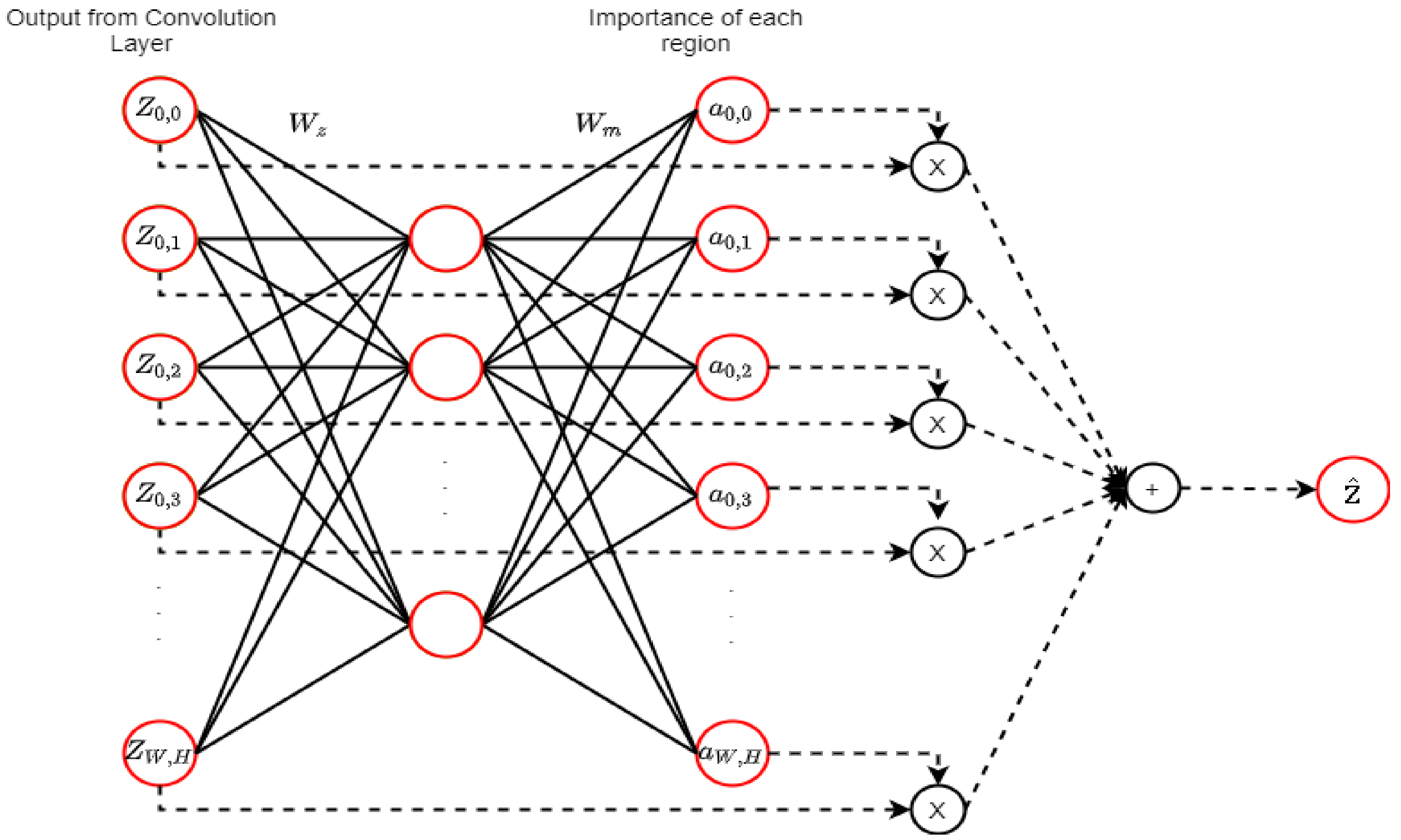
2.9. Attention Mechanism (AM)
An attention mechanism (AM) is a DL technique that was first introduced for language translation and performance enhancement that occurs by selecting significant features dynamically [51]. Figure 11 shows the attention mechanism in CNN that optimizes the weights and the biases to ensure the selection of important features in each region.
3. Summary of the lncRNAome Research Domains Where Deep Learning-Based Techniques Have Made Significant Contributions
Advances in next-generation sequencing techniques have afforded researchers the opportunity to study a plethora of novel lncRNA transcripts from multiple cells and tissues [17]. The state of lncRNA discovery and lncRNA annotation is still in its infancy. Several research groups are currently discovering new lncRNAs and applying different ML-based techniques to study different properties and functions of lncRNAs. In this section, we highlight different fields in the lncRNA research domain where DL-based techniques have been successfully used. An overview is given in Table 1.
3.1. LncRNA Identification
There are many existing methods for recognizing lncRNA transcripts which were developed based on shallow learning. For example, Lia et al. developed a tool called PLEK to recognize lncRNAs based on improved k-mer schemes [69]. Sun et al. developed the CNCI tool to distinguish lncRNA transcripts from protein-coding transcripts using the intrinsic composition of sequences [70]. An updated version of CNCI, called CNIT, which can provide the same solution with higher accuracy and faster speed has been produced [71].
Recently, due to the advancement of DL techniques, a lot of work has been published focusing on the identification of lncRNAs using DL-based techniques. For example, Tripath developed DeepLNC, a DNN-based network that uses k-mers (k = 1,2,3,4,5) from sequences as a feature set to distinguish lncRNA transcripts from mRNA transcripts [55]. Baek et al. developed lncRNAnet [52], which can be considered among the best of the performing models [72] for distinguishing full-length lncRNA transcripts from protein-coding transcripts. LncRNAnet used an RNN for sequence modeling and a CNN for the detection of stop codons to capture the open reading frame information. Yang et al. developed LncADeep, which can identify both partial and full-length lncRNA transcripts [53]. LncADeep incorporates different hand-curated features such as coding sequence (CDS) length, hexamer score, Fickett nucleotide features, etc. for developing a DBN-based model. In another recent publication, Liu et al. used k-mer embedding vectors for the sequences as input features and built the DL-based architecture using BLSTM and CNN [54]. Han et al. proposed an integrated platform for lncRNA recognition, which uses a sequence, structure, and physicochemical properties of sequences [73]. Interested readers may consult the review by Amin et al., which summarizes different DL-based methods that have been used to classify non-coding RNAs [72]. Table 2 provides a summary outcome from the articles that considered DL-based techniques to identify lncRNAs in multiple species.
As mentioned at the beginning of this section, many tools such as PLEK [69], CNCI [70], CNIT [71], etc. exist, and all of them were developed considering hand-curated features using traditional ML models for non-coding RNA identification. Interestingly, all the DL-based methods highlighted in Table 2 evaluated their proposed models against the traditional ML models and outperformed them for lncRNA identification, indicating the superiority of DL-based models over traditional ML models for this task.
3.2. Transcriptional Regulation of lncRNAs
To date, ML-based techniques have been used to detect underlying patterns in the promoter regions of lncRNAs and protein-coding genes [56,74,75]. Using an ML-based approach, Alam et al. showed that there are different sequence-specific patterns in the promoters of lncRNAs compared to the promoters of protein-coding genes. They also identified the list of transcription factors (TFs) that are involved in the transcriptional regulatory patterns specific to lncRNAs. Recently, Alam et al. developed a DL-based architecture, DeepCNPP, to distinguish the promoters of lncRNAs from the promoters of protein-coding genes ([56,74]. DeepCNPP was built using a CNN-based architecture and outperformed the existing models used for the same purpose. Alam et al. also developed a model, DeePEL, to distinguish between the transcription regulatory program of promoter-originated lncRNAs (p-lncRNA) and enhancer-originated lncRNAs (e-lncRNA) [57]. Table 3 provides a summary outcome from the articles that considered DL-based techniques to demystify the transcription regulation program for lncRNAs.
It is important to emphasize that the previous model [75] used for distinguishing the promoter of protein-coding genes and lncRNA genes incorporated hand-curated features based on the sequence of promoters, transcription factor binding sites at the promoter regions, CpG islands, repetitive elements, and epigenetic marks to achieve 81.69% accuracy on the classification task. On the other hand, the DL-based model, DeepCNPP [56], outperformed the previous model with 83.34% accuracy considering only the sequence-related information from the promoter of lncRNA genes.
3.3. Functional Annotation of lncRNAs
The functional annotation of lncRNA is a challenging task. There are many knowledge bases that collect the functionality of lncRNA based on the expression and/or the regulatory elements (transcription factors, transcription co-factors [76]) that are involved in their transcriptional regulation [20]. Some attempts to extract the known functionality of lncRNAs by literature mining have also been made [77].
Yang et al. developed LncADeep, a DNN-based architecture to infer the function of a lncRNA based on its interacting protein partners [53]. In lncADeep, Yang et al. used several sequence-and structure-related features from both lncRNA and proteins. These features were then fed into a DNN to predict lncRNA-protein interactions. To infer the function of lncRNAs, the authors used the Kyoto Encyclopedia of Genes and Genomes (KEGG) [78] and the Reactome [79] pathways enrichment of the predicted proteins. Since proteins usually work as functional modules [80], the authors also inferred the functional modules of lncRNAs based on interacting protein partners.
3.4. Predicting lncRNA Subcellular Localization
Cao et al. proposed an ensemble-based classifier to predict the location of lncRNAs in five subcellular locations: cytoplasm, cytosol, nucleus, ribosome, and exosome, yielding an overall performance accuracy of 59% [52,81]. Recently, Gudenas and Wang proposed the first DL-based localization predictor for lncRNAs. A DNN built only from sequence features is used to predict the subcellular localization of the lncRNAs, distinguishing between lncRNAs located in the nucleus and cytosol [58].
3.5. Predicting lncRNA–Protein Interactions
RNA binding proteins (RBP) play important roles in different biological processes [82] and are shown to be involved in different diseases, one of which is cancer [83]. With the advancement of sequencing technologies, RBP can be verified using cross-linking immunoprecipitation sequencing (CLIP-seq) [84]. However, these experiments are time-consuming and expensive. As an alternative, we can adopt a fast and affordable in silico approach using ML techniques for predicting RBP [85].
Many state-of-the-art tools for predicting lncRNA-protein interactions exist, such as lncPro [86], RPI-Pred [87], RPISeq-RF [88], etc., which were developed considering hand-curated features using traditional ML models. Among these tools, RPISeq-RF performed best for the task of lncRNA–protein prediction in many benchmark datasets [62]. Recently, DL-based architectures were used to predict lncRNA–protein interactions. For example, IPminer [59], RPI-SAN [60], and BGFE [61] are the tools where stacked auto-encoder networks were used to capture the important features of sequences, and then the learned features from the sequence were fed into random forest models to predict lncRNA-protein binding. Peng et al. developed a tool, RPITER [62], where they used stacked autoencoders and CNN to fit the k-mer sequence features and structure information from the RNA and protein.
Current methods have successfully predicted ncRNA and protein interactions with reasonably high accuracy, but most of the models were trained and tested on only small benchmark datasets mainly derived from ncRNA–protein complexes in a protein–RNA interaction database [89] or Protein Databank (PDB) [90]. Thus, there is a need for improving the generalization capability of these models. Interested readers may consult the review by Zhang et al. [91] for more details. Table 4 provides a summary outcome from the articles that considered DL-based techniques to predict lncRNA-protein interactions.
For lncRNA-protein interactions, multiple benchmark datasets exist (see Table 4) but there is no clear winner from the DL models (see Table 4) that performed the best in all benchmark datasets. For all benchmark datasets, there exists at least one DL-based model that outperformed the traditional ML-based models for the lncRNA–protein interaction prediction task. From the pool of conventional ML-based models, RPISeq-RF performed at a similar level of accuracy to the DL-based models in a few benchmark datasets [62]. Interested readers are encouraged to read the article by Yi et al. for more details [60].
3.6. Predicting lncRNA–miRNA Interactions
LncRNAs and microRNAs (miRNAs) interact with each other to form a complex regulatory network for controlling gene expression. Through this multi-level gene regulation (either transcriptional, post-transcriptional, or post-translational level), these two families of non-coding RNAs (miRNA and lncRNA) are involved in multiple aspects of cell cycles (e.g., cell division, cell differentiation, apoptosis). Recently, we witnessed an exponential growth of expression profiling of lncRNAs in different diseases and conditions, but information regarding lncRNA–miRNA interactions is still rare [92,93]. Huang et al. proposed the first large-scale lncRNA–miRNA predictive model using a network diffusion method on sequence information, expression profiles, and biological function ([93,94]). Similarly, Huang et al. proposed GCN-based model, graph convolution for novel lncRNA–miRNA interactions (GCLMI), to predict lncRNA–miRNA interactions [63]. Based on the proposed model, which combines graph convolution and an auto-encoder, Huang et al. found that the area under the curve (AUC) for the predictor was around 0.85, indicating that DL-based methods are important contributors in this research field.
3.7. Predicting lncRNA–DNA Binding
Prediction of lncRNA and DNA binding is a relatively new field of research. Until now, computational prediction of lncRNA–DNA interactions has received relatively little attention from the scientific community working in lncRNAome [95]. We did find several tools that assessed the triple helix formation of RNA–DNA interactions, namely Triplex [96], Triplex Domain Finder [97], Triplexator [98], Triplex-Inspector [99], and LongTarget [100].
Recently, Wang et al. proposed a DL-based model using different combinations of CNN and LSTM to predict the genome-wide DNA binding sites for twelve lncRNAs based on ChIRP-seq experimental data [64]. In that study, Wang et al. considered the best performing model to have two CNN layers and 32 kernels in each layer. The authors also concluded that LSTM-based models did not perform well, since long-range dependence along sequences is not necessary for lncRNA-DNA binding.
3.8. Predicting lncRNA-Disease Associations
There are many existing methods (e.g., Ping’s method [101], LDAP [102], SIMCLDA [103], MFLDA [104]) that have incorporated hand-curated features into traditional ML-based models to infer lncRNA–disease associations. Ping’s method and LDAP both consider similarity measures between lncRNAs and diseases to infer lncRNA-related diseases. Ping’s method also incorporates the topological information from the bipartite graph of the lncRNA–disease network to achieve better results than LDAP. On the other hand, SIMCLDA incorporates features from lncRNAs based on the Gaussian interaction profile kernels from lncRNA–disease interactions. SIMCLDA also incorporates features from diseases based on the Jaccard similarity of ontologies associated with diseases. Ping’s method and LDAP both performed better than SIMCLDA in benchmark datasets for multiple diseases [65]. MFLDA introduced a matrix factorization-based fusion model to predict lncRNA–disease associations. However, the performance of MFLDA was not as high compared to Ping’s method, LDAP, or SIMCLDA, as similarities between lncRNA and diseases were not incorporated into MFLDA [66].
Recently, Xuan et al. published a DL-based model called CNNLDA, a dual CNN with attention mechanisms for predicting lncRNA–disease associations [66]. CNNLDA integrates multiple sources of data considering similarities between diseases, similarities between lncRNAs, lncRNA–disease associations, disease–miRNA associations, and lncRNA–miRNA interactions under a single platform to outperform many of the state-of-the-art methods for predicting disease-related lncRNAs. Xual et al. also proposed another deep architecture, GCNLDA, which combines GCN and CNN to infer lncRNA–disease associations [65]. Hu et al. proposed NNLDA, a CNN-based DL architecture, that is used to predict the role of lncRNA in different diseases [67]. According to the authors, NNLDA was the first algorithm that considered deep neural networks for predicting lncRNA–disease associations. Table 5 provides a summary outcome from the articles that considered DL-based techniques to predict lncRNA–disease associations.
Compared to the traditional ML-based models (e.g., Ping’s method [101], LDAP [102], SIMCLDA [103], and MFLDA [104]), the DL-based models in Table 5 hugely improved the prediction of lncRNA–disease association. For example, CNNLDA outperformed Ping’s method, LDAP, SIMCLDA, and MFLDA by 8.05%, 8.85%, 20.6%, and 32.6%, respectively, in terms of AUC [66]. This clearly indicates the major contribution that DL-based models have made in the prediction of lncRNA–diseases associations.
3.9. Cancer Lassification
Mamun and Mondal proposed DL-based approaches to classify eight different cancer types using lncRNA expression profiles (RNA-seq) [68]. The authors discovered lncRNA expression to be a better signature compared to mRNA expression for classifying cancer types. Using four different types of deep neural networks (MLP, LSTM, CNN, and deep autoencoder (DAE)), the proposed models achieved an accuracy ranging from 94% to 98%.
4. Challenges for Deep Learning in lncRNA Research
In this section, we highlight some of the frequently encountered problems when building DL-based models for lncRNAome. We also briefly describe the problems and provide some recommendations to circumvent the issues.
4.1. Required Data Set Sizes
DL-based methods are most successful in supervised learning setups, where a sufficient number of samples are available for training the deep network. As a criterion, the number of training samples is expected to be as high as the number of total model parameters, although some regularization techniques can be used to avoid overfitting in cases of data scarcity [107]. LncRNAs are notoriously difficult to analyze, since their expression is low and cell-specific, making the number of lncRNAs from different cells and tissues available generally low. For image-based analysis, the training set can be augmented by different techniques such as rotation, scaling, or cropping [24]. However, for genomic sequences, the techniques are of a different type. For example, in the lncRNA–DNA binding prediction problem, Want et al. augmented the data by applying a random shift of genomic sequences either in the left or the right direction within a base pair range of 10 to 40 [64].
4.2. Imbalanced Datasets
Biological data are mostly imbalanced for training ML-based models [108]. There are many bioinformatics research problems where there is a need for handling such imbalanced data carefully, such as splice site predictions [109], poly (A) site predictions [110], protein–protein interaction motif findings [108], etc. Using imbalanced data for training DL-based models may result in undesirable or misleading results. To handle this issue, we need to follow specific criteria. First, we need to avoid using accuracy as an evaluation metric for models because accuracy is a misleading parameter for evaluating the performance of a model that uses imbalanced data. Instead of accuracy, we may use the area under the precision-recall curve (AUPRC), Matthews correlation coefficient (MCC), or F1-measure as a criterion for model evaluation. For example, in DeePEL, the DL-based model used to differentiate the transcription regulatory program between promoter-originated lncRNA (p-lncRNA) and enhancer-originated lncRNA (e-lncRNA), the authors mainly relied upon MCC as an evaluation metric since the dataset was imbalanced [57]. Additionally, instead of using cross-entropy loss, we may use weighted entropy loss, which penalizes the model for the misclassification of samples from the smaller class.
4.3. Interpreting and Visualizing Convolutional Networks
The interpretation of DL-based models is difficult [111]. Usually, DL-based models perform better than traditional ML-based models in terms of different evaluation metrics, which indicates that meaningful representations of data are learned by DL-based models. In terms of model explainability, the lowest-level (the level closest to the input data) representations are relatively simple to explain, but the higher-level features learned by different layers of DL-based models are difficult to interpret and can be considered to be a black box [112]. Opening this black box to interpret the high-level learned features will have a real impact on understanding the underlying biology of lncRNAs.
Feature importance scores can be used for the purpose of identifying the parts of an input that significantly contributed to achieving the result of the models. This can be done using two different methods: perturbation-based methods [113,114] and backpropagation-based methods [115,116]. For perturbation-based methods in sequence-based models, the input sequence is changed systematically (e.g., single-nucleotide substitution) to observe its impact on model performance. The main limitation of this approach is the high computational cost since we need to exhaustively search the perturbation. In backpropagation-based methods, the output signal is propagated backward from the output layer of the neural network to the input layer to check the contribution of different parts of the network. This approach is computationally more efficient and requires less time. For a more comprehensive discussion on model interpretability, readers may consult [117,118].
4.4. Model Selection and Model Building
There are many different types of DL architecture, and model selection is not a trivial task. The most commonly used network architectures are based on CNN and/or RNN. CNN architectures are mainly suited for high-dimensional data such as 2D images, 3D images, or higher numbers of genomic sequence data. RNN-based models can capture long-range dependencies from varying lengths of genomic sequence data. Sophisticated models can be developed by integrating multiple architectures into a novel architecture [109].
Determining the optimal structure of a deep network is also challenging. The optimal number of hidden layers and hidden units are problem-specific, and validation sets should be used to determine the optimal setup. More layers and hidden units in the neural network increase model complexity (number of representable functions), and discovering the local optimum becomes less prone to weight initialization [119].
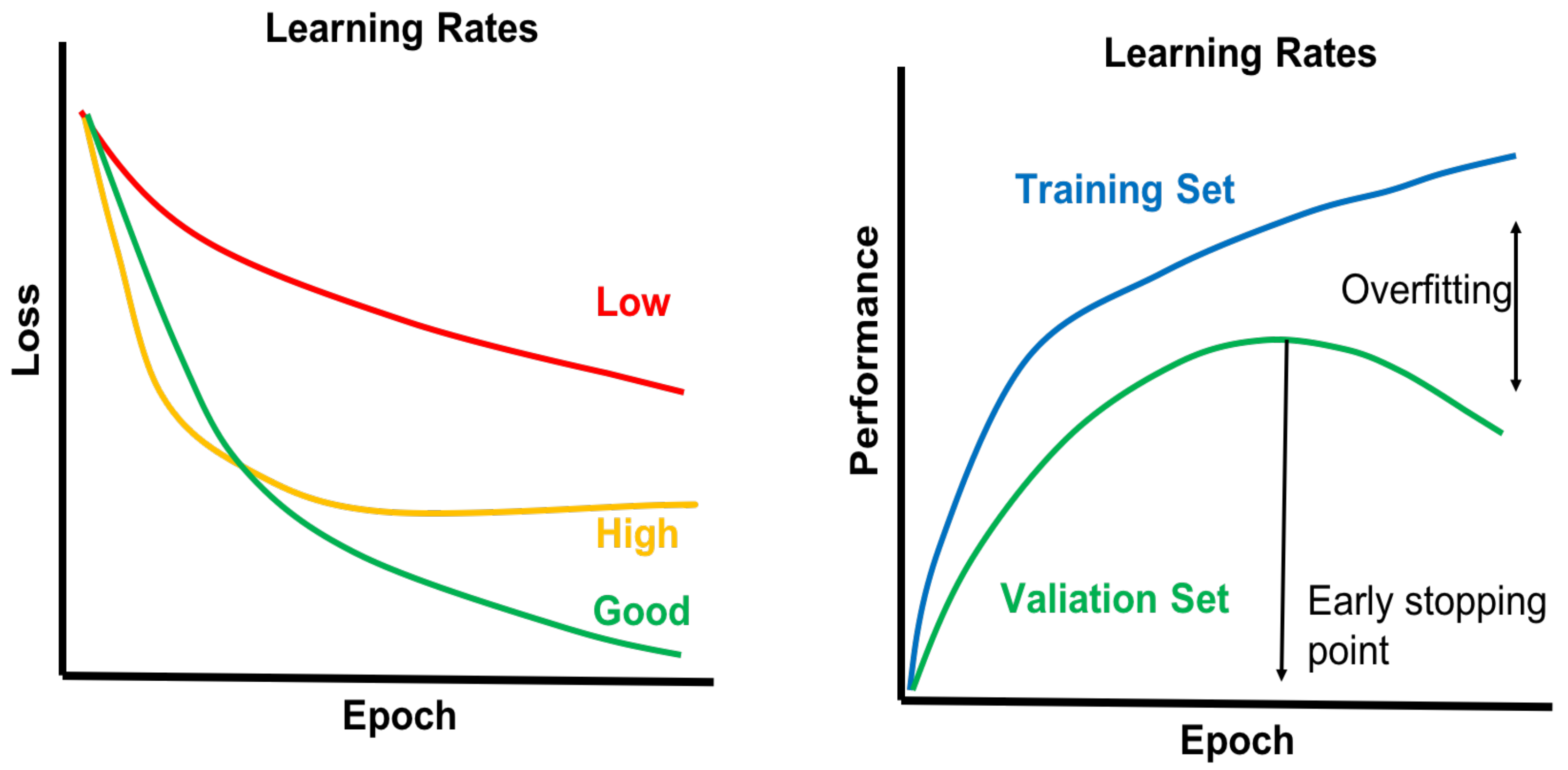
Training a deep network is far more complex and difficult than a shallow network [112]. Overfitting is a major challenge for training deep networks that result from using a model too complex for the data size of training sets. To avoid overfitting problems, the change of loss can be evaluated as a function of the number of epochs in the training phase. Depending on the learning rate value, the learning curve may change slowly or abruptly (Figure 12). Extreme learning rate values may result in a fluctuating learning curve [107]. Along with the loss function, monitoring the target performance parameter (e.g., accuracy, F1-score, etc.) is crucial for avoiding overfitting in both training sets and validation sets.
4.5. Confidence Score of the Prediction
In ML classification tasks, our main focus always revolves around the performance metric of the model. However, for real-life healthcare-related problems, we not only prefer a high prediction capability but also need to measure how confident the model is about its prediction, which enables us to evaluate the reliability of the model in clinical decision support systems, for example [120]. It is recommended that post-scaling be applied to Softmax output values from deep networks, as they are usually not on the right scale. Several methods have been proposed for the post-scaling purpose, such as temperate scaling [121], Platt scaling [122], isotonic regression [123], etc.
4.6. Catastrophic Forgetting
Catastrophic forgetting is a tendency of DL-based models to forget previously learned knowledge upon learning information from a new dataset [124]. Despite this, the integration of new lncRNA-related information is quite common, since new lncRNAs are constantly discovered and the information about known lncRNAs is increasing. For example, GENCODE release 21, published in 2014, contained 15,877 lncRNA genes. In 2019, this number increased to 17,904 lncRNA genes in GENCODE release 31. DL-based models that were developed based on earlier versions of data may not perform at the same level for newly released data. Training new models with new datasets are computationally exhaustive and time-consuming as well. There are different off-the-shelf solutions that may be used for this scenario such as dynamic neural networks with rehearsal training methods (e.g., Incremental Classifier and Representation Learning iCaRL [125]) and dual-memory-based learning systems [126].
5. Future Perspectives for Deep Learning in lncRNAome Research
DL-based methods are already extensively used in lncRNAs. However, to date, the most common DL architectures used in lnRNA-related research are CNN and RNN (see Table 1). Despite this, there are some other emerging architectures that may have applications in lncRNA-related research.
Di Lena et al. [127] applied deep spatio-temporal neural networks (DST-NNs) [128] using spatial features (e.g., protein secondary structures, orientation probabilities, and alignment probabilities) to determine protein structure predictions. Baldi et al. [129] applied multidimensional recurrent neural networks (MD-RNNs) [130] to amino acid sequences, the correlated profiles, and the secondary structures of proteins. Convolutional auto-encoders (CAEs) are designed to capitalize on the advantages of both CNN and AE to learn the hierarchical representation of data [131]. To the best of our knowledge, CAEs, MD-RNNs, and DST-NNs have not yet been used in the lncRNA domain.
Graph convolutional networks (GCN) have been successfully used in predicting different molecular attributes such as solubility, drug efficacy, etc. Recently, GCN and attention-based mechanisms have been used in lncRNA–disease prediction [65]. However, GCN, or attention-based mechanisms, have not been used in lncRNA–protein predictions thus far, and this might be an interesting area for further research.
GAN belongs to unsupervised learning methods, where the goal is to discover the underlying patterns from the data. GAN can also generate new sample data (e.g., sequences) with some variations. To date, the application of GAN is mainly focused on image processing [43]. However, as a relatively new method, the application of GAN is extremely limited in genomics. GAN models have been used to generate protein-coding DNA sequences [132] as well as for designing DNA probes for protein binding microarrays but have not been used in lncRNA research.
Capsule network models are a relatively new invention in the DL domain [133]. These models attempt to mimic the hierarchical representation of the human brain. Recently, capsule network models have been successfully used to classify brain tumor images [134]. However, capsule networks have not been used in any significant application in the lncRNA domain. LncRNAome might be an interesting area for capsule network-based research.
6. Conclusions
In this article, we summarized the contribution of DL in nine different lncRNAome research areas and highlighted the challenges DL-based researchers may face while developing models for lncRNAome. Comparative results from DL- and ML-based models highlight DL-based models’ superiority in different lncRNAome prediction tasks. Specifically, in the study of lncRNA identification, the distinction of transcription regulation programs for lncRNA, lncRNA–protein interaction prediction, and lncRNA–disease association prediction, DL-based models have outperformed the traditional ML-based models. Based on these results, there is significant potential for the application of DL-based techniques in lncRNAome. Unfortunately, only a few DL-based models for the task of lncRNA localization prediction, lncRNA–DNA interaction prediction, and the distinction of transcription regulation program for lncRNA exist. Researchers should consider focusing on developing new DL-based models in these areas which have received relatively little attention from the scientific community. However, the development of DL-based models for lncRNAome is a daunting task. Due to the low expression level and cell-/tissue-specific nature of lncRNA, DL-based model development may need to overcome the challenges of utilizing a relatively smaller dataset while building cell-/tissue-specific models. Additionally, the evolving annotations of lncRNAs from multiple research groups orchestrate another layer of complication in integrating newly discovered lncRNA into existing models. Thus, in spite of DL-based models achieving high-level prediction accuracy thus far, huge challenges in applying DL-based models in lncRNAome still exist. Leveraging state-of-the-art DL-based techniques while improving the existing ones, we expect to gain a better insight into lncRNAome in the near future.
Funding
The open access publication of this article was funded by the College of Science and Engineering, Hamad Bin Khalifa University, Doha, Qatar.
Conflicts of Interest
The authors declare no conflict of interest.
References
- Quinn, J.J.; Chang, H.Y. Unique features of long non-coding RNA biogenesis and function. Nat. Rev. Genet. 2016, 17, 47–62. [Google Scholar] [CrossRef]
- International Human Genome Sequencing Consortium. Initial sequencing and analysis of the human genome. Nature 2001, 409, 860–921. [Google Scholar] [CrossRef] [PubMed] [Green Version]
- Wapinski, O.; Chang, H.Y. Long noncoding RNAs and human disease. Trends Cell Biol. 2011, 21, 354–361. [Google Scholar] [CrossRef] [PubMed]
- Kino, T.; Hurt, D.E.; Ichijo, T.; Nader, N.; Chrousos, G.P. Noncoding RNA gas5 is a growth arrest- and starvation-associated repressor of the glucocorticoid receptor. Sci. Signal. 2010, 3, ra8. [Google Scholar] [CrossRef] [PubMed] [Green Version]
- Mourtada-Maarabouni, M.; Pickard, M.R.; Hedge, V.L.; Farzaneh, F.; Williams, G.T. GAS5, a non-protein-coding RNA, controls apoptosis and is downregulated in breast cancer. Oncogene 2009, 28, 195–208. [Google Scholar] [CrossRef] [PubMed] [Green Version]
- Shi, X.; Sun, M.; Liu, H.; Yao, Y.; Song, Y. Long non-coding RNAs: A new frontier in the study of human diseases. Cancer Lett. 2013, 339, 159–166. [Google Scholar] [CrossRef]
- Huang, Y.; Regazzi, R.; Cho, W. Emerging Roles of Long Noncoding RNAs in Neurological Diseases and Metabolic Disorders; Frontiers Media SAP: Lausanne, Switzerland, 2015; ISBN 9782889195718. [Google Scholar]
- Lin, N.; Rana, T.M. Dysregulation of Long Non-coding RNAs in Human Disease. In Molecular Biology of Long Non-Coding RNAs; Springer: Berlin/Heidelberg, Germany, 2013; pp. 115–136. [Google Scholar]
- Jarroux, J.; Morillon, A.; Pinskaya, M. History, Discovery, and Classification of lncRNAs. Adv. Exp. Med. Biol. 2017, 1008, 1–46. [Google Scholar]
- Brannan, C.I.; Dees, E.C.; Ingram, R.S.; Tilghman, S.M. The product of the H19 gene may function as an RNA. Mol. Cell. Biol. 1990, 10, 28–36. [Google Scholar] [CrossRef] [Green Version]
- Lyon, M.F. Gene Action in the X-chromosome of the Mouse (Mus musculus L.). Nature 1961, 190, 372–373. [Google Scholar] [CrossRef]
- Brown, C.J.; Ballabio, A.; Rupert, J.L.; Lafreniere, R.G.; Grompe, M.; Tonlorenzi, R.; Willard, H.F. A gene from the region of the human X inactivation centre is expressed exclusively from the inactive X chromosome. Nature 1991, 349, 38–44. [Google Scholar] [CrossRef]
- Brockdorff, N.; Ashworth, A.; Kay, G.F.; Cooper, P.; Smith, S.; McCabe, V.M.; Norris, D.P.; Penny, G.D.; Patel, D.; Rastan, S. Conservation of position and exclusive expression of mouse Xist from the inactive X chromosome. Nature 1991, 351, 329–331. [Google Scholar] [CrossRef] [PubMed]
- Orgel, L.E.; Crick, F.H. Selfish DNA: The ultimate parasite. Nature 1980, 284, 604–607. [Google Scholar] [CrossRef] [PubMed]
- The FANTOM Consortium and the RIKEN Genome Exploration Research Group Phase I & II Team. The Transcriptional Landscape of the Mammalian Genome. Science 2005, 309, 1559–1563. [Google Scholar] [CrossRef] [PubMed] [Green Version]
- The FANTOM Consortium and the RIKEN Genome Exploration Research Group Phase I & II Team. Analysis of the mouse transcriptome based on functional annotation of 60,770 full-length cDNAs. Nature 2002, 420, 563–573. [Google Scholar] [CrossRef] [Green Version]
- Hon, C.-C.; Ramilowski, J.A.; Harshbarger, J.; Bertin, N.; Rackham, O.J.L.; Gough, J.; Denisenko, E.; Schmeier, S.; Poulsen, T.M.; Severin, J.; et al. An atlas of human long non-coding RNAs with accurate 5′ ends. Nature 2017, 543, 199–204. [Google Scholar] [CrossRef] [Green Version]
- Derrien, T.; Johnson, R.; Bussotti, G.; Tanzer, A.; Djebali, S.; Tilgner, H.; Guernec, G.; Martin, D.; Merkel, A.; Knowles, D.G.; et al. The GENCODE v7 catalog of human long noncoding RNAs: Analysis of their gene structure, evolution, and expression. Genome Res. 2012, 22, 1775–1789. [Google Scholar] [CrossRef] [Green Version]
- Iyer, M.K.; Niknafs, Y.S.; Malik, R.; Singhal, U.; Sahu, A.; Hosono, Y.; Barrette, T.R.; Prensner, J.R.; Evans, J.R.; Zhao, S.; et al. The landscape of long noncoding RNAs in the human transcriptome. Nat. Genet. 2015, 47, 199–208. [Google Scholar] [CrossRef]
- Alam, T.; Uludag, M.; Essack, M.; Salhi, A.; Ashoor, H.; Hanks, J.B.; Kapfer, C.; Mineta, K.; Gojobori, T.; Bajic, V.B. FARNA: Knowledgebase of inferred functions of non-coding RNA transcripts. Nucleic Acids Res. 2017, 45, 2838–2848. [Google Scholar] [CrossRef]
- Eraslan, G.; Avsec, Ž.; Gagneur, J.; Theis, F.J. Deep learning: New computational modelling techniques for genomics. Nat. Rev. Genet. 2019, 20, 389–403. [Google Scholar] [CrossRef]
- Chen, L.-C.; Papandreou, G.; Kokkinos, I.; Murphy, K.; Yuille, A.L. DeepLab: Semantic Image Segmentation with Deep Convolutional Nets, Atrous Convolution, and Fully Connected CRFs. IEEE Trans. Pattern Anal. Mach. Intell. 2018, 40, 834–848. [Google Scholar] [CrossRef]
- Bengio, Y.; Courville, A.; Vincent, P. Representation learning: A review and new perspectives. IEEE Trans. Pattern Anal. Mach. Intell. 2013, 35, 1798–1828. [Google Scholar] [CrossRef] [PubMed]
- Krizhevsky, A.; Sutskever, I.; Hinton, G.E. ImageNet classification with deep convolutional neural networks. Commun. ACM 2017, 60, 84–90. [Google Scholar] [CrossRef]
- Wu, Y.; Schuster, M.; Chen, Z.; Le, Q.V.; Norouzi, M.; Macherey, W.; Krikun, M.; Cao, Y.; Gao, Q.; Macherey, K.; et al. Google’s Neural Machine Translation System: Bridging the Gap between Human and Machine Translation. arXiv 2016, arXiv:1609.08144. [Google Scholar]
- Amodei, D.; Ananthanarayanan, S.; Anubhai, R.; Bai, J.; Battenberg, E.; Case, C.; Casper, J.; Catanzaro, B.; Cheng, Q.; Chen, G.; et al. Deep Speech 2: End-to-End Speech Recognition in English and Mandarin. In Proceedings of the International Conference on Machine Learning, New York, NY, USA, 19–24 June 2016; pp. 173–182. [Google Scholar]
- Khan, S.H.; Hayat, M.; Porikli, F. Regularization of deep neural networks with spectral dropout. Neural Netw. 2019, 110, 82–90. [Google Scholar] [CrossRef] [Green Version]
- Xiong, J.; Zhang, K.; Zhang, H. A Vibrating Mechanism to Prevent Neural Networks from Overfitting. In Proceedings of the 15th International Wireless Communications & Mobile Computing Conference (IWCMC), Tangier, Morocco, 24–28 June 2019. [Google Scholar]
- Min, S.; Lee, B.; Yoon, S. Deep learning in bioinformatics. Brief. Bioinform. 2017, 18, 851–869. [Google Scholar] [CrossRef] [Green Version]
- Hinton, G.E. How neural networks learn from experience. Sci. Am. 1992, 267, 144–151. [Google Scholar] [CrossRef]
- LeCun, Y.; Bengio, Y.; Hinton, G. Deep learning. Nature 2015, 521, 436–444. [Google Scholar] [CrossRef]
- Goldberg, Y. Neural Network Methods for Natural Language Processing. Synth. Lect. Hum. Lang. Technol. 2017, 10, 1–309. [Google Scholar] [CrossRef]
- University of Colorado, Deptartment of Computer Science; Smolensky, P. Information Processing in Dynamical Systems: Foundations of Harmony Theory; MIT Press: Cambridge, MA, USA, 1986. [Google Scholar]
- Sugiyama, M. Statistical Machine Learning. In Introduction to Statistical Machine Learning; Elsevier: Amsterdam, The Netherlands, 2016; pp. 3–8. [Google Scholar]
- Hinton, G. Deep belief networks. Scholarpedia 2009, 4, 5947. [Google Scholar] [CrossRef]
- Karhunen, J.; Raiko, T.; Cho, K. Unsupervised deep learning. In Advances in Independent Component Analysis and Learning Machines; Elsevier: Amsterdam, The Netherlands, 2015; pp. 125–142. [Google Scholar]
- Albawi, S.; Mohammed, T.A.; Al-Zawi, S. Understanding of a convolutional neural network. In Proceedings of the International Conference on Engineering and Technology (ICET), Antalya, Turkey, 21–23 August 2017. [Google Scholar]
- Lin, M.; Chen, Q.; Yan, S. Network in Network. arXiv 2013, arXiv:1312.4400. [Google Scholar]
- Alom, M.Z.; Taha, T.M.; Yakopcic, C.; Westberg, S.; Sidike, P.; Nasrin, M.S.; Hasan, M.; van Essen, B.C.; Awwal, A.A.S.; Asari, V.K. A State-of-the-Art Survey on Deep Learning Theory and Architectures. Electronics 2019, 8, 292. [Google Scholar] [CrossRef] [Green Version]
- Zhang, S.; Tong, H.; Xu, J.; Maciejewski, R. Graph convolutional networks: A comprehensive review. Comput. Soc. Netw. 2019, 6, 11. [Google Scholar] [CrossRef] [Green Version]
- Graph Convolutional Networks. Available online: https://tkipf.github.io/graph-convolutional-networks/ (accessed on 24 July 2020).
- Zhu, L.; Chen, Y.; Ghamisi, P.; Benediktsson, J.A. Generative Adversarial Networks for Hyperspectral Image Classification. IEEE Trans. Geosci. Remote Sens. 2018, 56, 5046–5063. [Google Scholar] [CrossRef]
- Goodfellow, I.; Pouget-Abadie, J.; Mirza, M.; Xu, B.; Warde-Farley, D.; Ozair, S.; Courville, A.; Bengio, Y. Generative Adversarial Nets. In Proceedings of the Advances in Neural Information Processing Systems, Montreal, QC, Canada, 8–13 December 2014; pp. 2672–2680. [Google Scholar]
- Blaschke, T.; Olivecrona, M.; Engkvist, O.; Bajorath, J.; Chen, H. Application of Generative Autoencoder in De Novo Molecular Design. Mol. Inform. 2018, 37. [Google Scholar] [CrossRef] [PubMed] [Green Version]
- Luo, X.; Li, X.; Wang, Z.; Liang, J. Discriminant autoencoder for feature extraction in fault diagnosis. Chemom. Intell. Lab. Syst. 2019, 192, 103814. [Google Scholar] [CrossRef]
- Schuster, M.; Paliwal, K.K. Bidirectional recurrent neural networks. IEEE Trans. Signal Process. 1997, 45, 2673–2681. [Google Scholar] [CrossRef] [Green Version]
- Sterzing, V.; Schurmann, B. Recurrent neural networks for temporal learning of time series. In Proceedings of the IEEE International Conference on Neural Networks, San Francisco, CA, USA, 28 March–1 April 1993; pp. 843–850. [Google Scholar]
- Greff, K.; Srivastava, R.K.; Koutnik, J.; Steunebrink, B.R.; Schmidhuber, J. LSTM: A Search Space Odyssey. IEEE Trans. Neural Netw. Learn. Syst. 2017, 28, 2222–2232. [Google Scholar] [CrossRef] [PubMed] [Green Version]
- Azzouni, A.; Pujolle, G. A Long Short-Term Memory Recurrent Neural Network Framework for Network Traffic Matrix Prediction. arXiv 2017, arXiv:1705.05690. [Google Scholar]
- Bidirectional Recurrent Neural Networks—IEEE Journals & Magazine. Available online: https://0-ieeexplore-ieee-org.brum.beds.ac.uk/document/650093 (accessed on 18 September 2020).
- Yakura, H.; Shinozaki, S.; Nishimura, R.; Oyama, Y.; Sakuma, J. Neural malware analysis with attention mechanism. Comput. Secur. 2019, 87, 101592. [Google Scholar] [CrossRef]
- Baek, J.; Lee, B.; Kwon, S.; Yoon, S. LncRNAnet: Long non-coding RNA identification using deep learning. Bioinformatics 2018, 34, 3889–3897. [Google Scholar] [CrossRef] [PubMed]
- Yang, C.; Yang, L.; Zhou, M.; Xie, H.; Zhang, C.; Wang, M.D.; Zhu, H. LncADeep: An ab initio lncRNA identification and functional annotation tool based on deep learning. Bioinformatics 2018, 34, 3825–3834. [Google Scholar] [CrossRef] [PubMed]
- Liu, X.-Q.; Li, B.-X.; Zeng, G.-R.; Liu, Q.-Y.; Ai, D.-M. Prediction of Long Non-Coding RNAs Based on Deep Learning. Genes 2019, 10. [Google Scholar] [CrossRef] [PubMed] [Green Version]
- Tripathi, R.; Patel, S.; Kumari, V.; Chakraborty, P.; Varadwaj, P.K. DeepLNC, a long non-coding RNA prediction tool using deep neural network. Netw. Model. Anal. Health Inform. Bioinform. 2016, 5, 21. [Google Scholar] [CrossRef]
- Alam, T.; Islam, M.T.; Househ, M.; Belhaouari, S.B.; Kawsar, F.A. DeepCNPP: Deep Learning Architecture to Distinguish the Promoter of Human Long Non-Coding RNA Genes and Protein-Coding Genes. Stud. Health Technol. Inform. 2019, 262, 232–235. [Google Scholar]
- Alam, T.; Islam, M.T.; Schmeier, S.; Househ, M.; Al-Thani, D.A. DeePEL: Deep learning architecture to recognize p-lncRNA and e-lncRNA promoters. In Proceedings of the IEEE International Conference on Bioinformatics and Biomedicine (BIBM), San Diego, CA, USA, 18–21 November 2019. [Google Scholar]
- Gudenas, B.L.; Wang, L. Prediction of LncRNA Subcellular Localization with Deep Learning from Sequence Features. Sci. Rep. 2018, 8, 1–10. [Google Scholar] [CrossRef] [Green Version]
- Pan, X.; Fan, Y.-X.; Yan, J.; Shen, H.-B. IPMiner: Hidden ncRNA-protein interaction sequential pattern mining with stacked autoencoder for accurate computational prediction. BMC Genom. 2016, 17, 582. [Google Scholar] [CrossRef] [Green Version]
- Yi, H.-C.; You, Z.-H.; Huang, D.-S.; Li, X.; Jiang, T.-H.; Li, L.-P. A Deep Learning Framework for Robust and Accurate Prediction of ncRNA-Protein Interactions Using Evolutionary Information. Mol. Ther. Nucleic Acids 2018, 11, 337–344. [Google Scholar] [CrossRef] [Green Version]
- Zhan, Z.-H.; Jia, L.-N.; Zhou, Y.; Li, L.-P.; Yi, H.-C. BGFE: A Deep Learning Model for ncRNA-Protein Interaction Predictions Based on Improved Sequence Information. Int. J. Mol. Sci. 2019, 20. [Google Scholar] [CrossRef] [Green Version]
- Peng, C.; Han, S.; Zhang, H.; Li, Y. RPITER: A Hierarchical Deep Learning Framework for ncRNA–Protein Interaction Prediction. Int. J. Mol. Sci. 2019, 20, 1070. [Google Scholar] [CrossRef] [Green Version]
- Huang, Y.-A.; Huang, Z.-A.; You, Z.-H.; Zhu, Z.; Huang, W.-Z.; Guo, J.-X.; Yu, C.-Q. Predicting lncRNA-miRNA Interaction via Graph Convolution Auto-Encoder. Front. Genet. 2019, 10, 758. [Google Scholar] [CrossRef] [Green Version]
- Wang, F.; Chainani, P.; White, T.; Yang, J.; Liu, Y.; Soibam, B. Deep learning identifies genome-wide DNA binding sites of long noncoding RNAs. RNA Biol. 2018, 15, 1468–1476. [Google Scholar] [CrossRef] [PubMed]
- Xuan, P.; Pan, S.; Zhang, T.; Liu, Y.; Sun, H. Graph Convolutional Network and Convolutional Neural Network Based Method for Predicting lncRNA-Disease Associations. Cells 2019, 8. [Google Scholar] [CrossRef] [PubMed] [Green Version]
- Xuan, P.; Cao, Y.; Zhang, T.; Kong, R.; Zhang, Z. Dual Convolutional Neural Networks with Attention Mechanisms Based Method for Predicting Disease-Related lncRNA Genes. Front. Genet. 2019, 10, 416. [Google Scholar] [CrossRef] [PubMed] [Green Version]
- Hu, J. Deep learning enables accurate prediction of interplay between lncRNA and disease. Front. Genet. 2019, 10. [Google Scholar] [CrossRef] [PubMed]
- Mamun, A.A.; Al Mamun, A.; Mondal, A.M. Long Non-coding RNA Based Cancer Classification using Deep Neural Networks. In Proceedings of the 10th ACM International Conference on Bioinformatics, Computational Biology and Health Informatics—BCB ’19, Niagara Falls, NY, USA, 7–10 September 2019. [Google Scholar]
- Li, A.; Zhang, J.; Zhou, Z. PLEK: A tool for predicting long non-coding RNAs and messenger RNAs based on an improved k-mer scheme. BMC Bioinform. 2014, 15, 311. [Google Scholar] [CrossRef] [Green Version]
- Sun, L.; Luo, H.; Bu, D.; Zhao, G.; Yu, K.; Zhang, C.; Liu, Y.; Chen, R.; Zhao, Y. Utilizing sequence intrinsic composition to classify protein-coding and long non-coding transcripts. Nucleic Acids Res. 2013, 41, e166. [Google Scholar] [CrossRef]
- Guo, J.-C.; Fang, S.-S.; Wu, Y.; Zhang, J.-H.; Chen, Y.; Liu, J.; Wu, B.; Wu, J.-R.; Li, E.-M.; Xu, L.-Y.; et al. CNIT: A fast and accurate web tool for identifying protein-coding and long non-coding transcripts based on intrinsic sequence composition. Nucleic Acids Res. 2019, 47, W516–W522. [Google Scholar] [CrossRef] [Green Version]
- Amin, N.; McGrath, A.; Chen, Y.-P.P. Evaluation of deep learning in non-coding RNA classification. Nat. Mach. Intell. 2019, 1, 246–256. [Google Scholar] [CrossRef]
- Han, S.; Liang, Y.; Ma, Q.; Xu, Y.; Zhang, Y.; Du, W.; Wang, C.; Li, Y. LncFinder: An integrated platform for long non-coding RNA identification utilizing sequence intrinsic composition, structural information and physicochemical property. Brief. Bioinform. 2018, 20, 2009–2027. [Google Scholar] [CrossRef]
- Lin, J.; Wen, Y.; He, S.; Yang, X.; Zhang, H.; Zhu, H. Pipelines for cross-species and genome-wide prediction of long noncoding RNA binding. Nat. Protoc. 2019, 14, 795–818. [Google Scholar] [CrossRef]
- Alam, T.; Medvedeva, Y.A.; Jia, H.; Brown, J.B.; Lipovich, L.; Bajic, V.B. Promoter analysis reveals globally differential regulation of human long non-coding RNA and protein-coding genes. PLoS ONE 2014, 9, e109443. [Google Scholar] [CrossRef] [PubMed] [Green Version]
- Schmeier, S.; Alam, T.; Essack, M.; Bajic, V.B. TcoF-DB v2: Update of the database of human and mouse transcription co-factors and transcription factor interactions. Nucleic Acids Res. 2017, 45, D145–D150. [Google Scholar] [CrossRef] [PubMed] [Green Version]
- Salhi, A.; Essack, M.; Alam, T.; Bajic, V.P.; Ma, L.; Radovanovic, A.; Marchand, B.; Schmeier, S.; Zhang, Z.; Bajic, V.B. DES-ncRNA: A knowledgebase for exploring information about human micro and long noncoding RNAs based on literature-mining. RNA Biol. 2017, 14, 963–971. [Google Scholar] [CrossRef]
- Kanehisa, M. KEGG: Kyoto Encyclopedia of Genes and Genomes. Nucleic Acids Res. 2000, 28, 27–30. [Google Scholar] [CrossRef] [PubMed]
- Fabregat, A.; Jupe, S.; Matthews, L.; Sidiropoulos, K.; Gillespie, M.; Garapati, P.; Haw, R.; Jassal, B.; Korninger, F.; May, B.; et al. The Reactome Pathway Knowledgebase. Nucleic Acids Res. 2018, 46, D649–D655. [Google Scholar] [CrossRef] [PubMed]
- Enright, A.J.; Van Dongen, S.; Ouzounis, C.A. An efficient algorithm for large-scale detection of protein families. Nucleic Acids Res. 2002, 30, 1575–1584. [Google Scholar] [CrossRef]
- Cao, Z.; Pan, X.; Yang, Y.; Huang, Y.; Shen, H.-B. The lncLocator: A subcellular localization predictor for long non-coding RNAs based on a stacked ensemble classifier. Bioinformatics 2018, 34, 2185–2194. [Google Scholar] [CrossRef]
- Glisovic, T.; Bachorik, J.L.; Yong, J.; Dreyfuss, G. RNA-binding proteins and post-transcriptional gene regulation. FEBS Lett. 2008, 582, 1977–1986. [Google Scholar] [CrossRef] [Green Version]
- Kim, M.Y.; Hur, J.; Jeong, S. Emerging roles of RNA and RNA-binding protein network in cancer cells. BMB Rep. 2009, 42, 125–130. [Google Scholar] [CrossRef] [Green Version]
- Li, J.-H.; Liu, S.; Zhou, H.; Qu, L.-H.; Yang, J.-H. starBase v2.0: Decoding miRNA-ceRNA, miRNA-ncRNA and protein-RNA interaction networks from large-scale CLIP-Seq data. Nucleic Acids Res. 2014, 42, D92–D97. [Google Scholar] [CrossRef] [Green Version]
- Pan, X.; Shen, H.-B. Predicting RNA–protein binding sites and motifs through combining local and global deep convolutional neural networks. Bioinformatics 2018, 34, 3427–3436. [Google Scholar] [CrossRef] [PubMed] [Green Version]
- Lu, Q.; Ren, S.; Lu, M.; Zhang, Y.; Zhu, D.; Zhang, X.; Li, T. Computational prediction of associations between long non-coding RNAs and proteins. BMC Genom. 2013, 14, 651. [Google Scholar] [CrossRef] [PubMed] [Green Version]
- Suresh, V.; Liu, L.; Adjeroh, D.; Zhou, X. RPI-Pred: Predicting ncRNA-protein interaction using sequence and structural information. Nucleic Acids Res. 2015, 43, 1370–1379. [Google Scholar] [CrossRef] [PubMed] [Green Version]
- Muppirala, U.K.; Honavar, V.G.; Dobbs, D. Predicting RNA-protein interactions using only sequence information. BMC Bioinform. 2011, 12, 489. [Google Scholar] [CrossRef] [PubMed] [Green Version]
- Lewis, B.A.; Walia, R.R.; Terribilini, M.; Ferguson, J.; Zheng, C.; Honavar, V.; Dobbs, D. PRIDB: A Protein-RNA interface database. Nucleic Acids Res. 2011, 39, D277–D282. [Google Scholar] [CrossRef] [PubMed] [Green Version]
- Berman, H.; Westbrook, J.; Feng, Z.; Gilliland, G.; Bhat, T.; Weissig, H.; Shindyalov, I.; Bourne, P. The Protein Data Bank. Nucleic Acids Res. 2000, 28, 235–242. [Google Scholar] [CrossRef] [PubMed] [Green Version]
- Zhang, S.-W.; Fan, X.-N. Computational Methods for Predicting ncRNA-protein Interactions. Med. Chem. 2017, 13, 515–525. [Google Scholar] [CrossRef]
- Zheng, Y.; Li, T.; Xu, Z.; Wai, C.M.; Chen, K.; Zhang, X.; Wang, S.; Ji, B.; Ming, R.; Sunkar, R. Identification of microRNAs, phasiRNAs and Their Targets in Pineapple. Trop. Plant Biol. 2016, 9, 176–186. [Google Scholar] [CrossRef]
- Jalali, S.; Bhartiya, D.; Lalwani, M.K.; Sivasubbu, S.; Scaria, V. Systematic transcriptome wide analysis of lncRNA-miRNA interactions. PLoS ONE 2013, 8, e53823. [Google Scholar] [CrossRef] [Green Version]
- Huang, Z.-A.; Huang, Y.-A.; You, Z.-H.; Zhu, Z.; Sun, Y. Novel link prediction for large-scale miRNA-lncRNA interaction network in a bipartite graph. BMC Med. Genom. 2018, 11, 17–27. [Google Scholar] [CrossRef] [Green Version]
- Antonov, I.V.; Mazurov, E.; Borodovsky, M.; Medvedeva, Y.A. Prediction of lncRNAs and their interactions with nucleic acids: Benchmarking bioinformatics tools. Brief. Bioinform. 2019, 20, 551–564. [Google Scholar] [CrossRef] [PubMed]
- Hon, J.; Martínek, T.; Rajdl, K.; Lexa, M. Triplex: An R/Bioconductor package for identification and visualization of potential intramolecular triplex patterns in DNA sequences. Bioinformatics 2013, 29, 1900–1901. [Google Scholar] [CrossRef] [PubMed] [Green Version]
- Hänzelmann, S.; Kuo, C.-C.; Kalwa, M.; Wagner, W.; Costa, I.G. Triplex Domain Finder: Detection of Triple Helix Binding Domains in Long Non-Coding RNAs. bioRxiv 2015. [Google Scholar] [CrossRef]
- Buske, F.A.; Bauer, D.C.; Mattick, J.S.; Bailey, T.L. Triplexator: Detecting nucleic acid triple helices in genomic and transcriptomic data. Genome Res. 2012, 22, 1372–1381. [Google Scholar] [CrossRef] [PubMed] [Green Version]
- Buske, F.A.; Bauer, D.C.; Mattick, J.S.; Bailey, T.L. Triplex-Inspector: An analysis tool for triplex-mediated targeting of genomic loci. Bioinformatics 2013, 29, 1895–1897. [Google Scholar] [CrossRef] [Green Version]
- He, S.; Zhang, H.; Liu, H.; Zhu, H. LongTarget: A tool to predict lncRNA DNA-binding motifs and binding sites via Hoogsteen base-pairing analysis. Bioinformatics 2015, 31, 178–186. [Google Scholar] [CrossRef] [Green Version]
- Ping, P.; Wang, L.; Kuang, L.; Ye, S.; Iqbal, M.F.B.; Pei, T. A Novel Method for LncRNA-Disease Association Prediction Based on an lncRNA-Disease Association Network. IEEE/ACM Trans. Comput. Biol. Bioinform. 2019, 16, 688–693. [Google Scholar] [CrossRef]
- Lan, W.; Li, M.; Zhao, K.; Liu, J.; Wu, F.-X.; Pan, Y.; Wang, J. LDAP: A web server for lncRNA-disease association prediction. Bioinformatics 2017, 33, 458–460. [Google Scholar] [CrossRef]
- Lu, C.; Yang, M.; Luo, F.; Wu, F.-X.; Li, M.; Pan, Y.; Li, Y.; Wang, J. Prediction of lncRNA-disease associations based on inductive matrix completion. Bioinformatics 2018, 34, 3357–3364. [Google Scholar] [CrossRef] [Green Version]
- Fu, G.; Wang, J.; Domeniconi, C.; Yu, G. Matrix factorization-based data fusion for the prediction of lncRNA-disease associations. Bioinformatics 2018, 34, 1529–1537. [Google Scholar] [CrossRef]
- Chen, X.; Yan, C.C.; Luo, C.; Ji, W.; Zhang, Y.; Dai, Q. Constructing lncRNA functional similarity network based on lncRNA-disease associations and disease semantic similarity. Sci. Rep. 2015, 5, 11338. [Google Scholar] [CrossRef] [PubMed] [Green Version]
- Wang, D.; Wang, J.; Lu, M.; Song, F.; Cui, Q. Inferring the human microRNA functional similarity and functional network based on microRNA-associated diseases. Bioinformatics 2010, 26, 1644–1650. [Google Scholar] [CrossRef] [PubMed] [Green Version]
- Bengio, Y. Practical Recommendations for Gradient-Based Training of Deep Architectures. Lect. Notes Comput. Sci. 2012, 7700, 437–478. [Google Scholar]
- Alam, T.; Alazmi, M.; Naser, R.; Huser, F.; Momin, A.A.; Walkiewicz, K.W.; Canlas, C.G.; Huser, R.G.; Ali, A.J.; Merzaban, J.; et al. Proteome-level assessment of origin, prevalence and function of Leucine-Aspartic Acid (LD) motifs. Bioinformatics 2020, 36, 1121–1128. [Google Scholar] [CrossRef] [PubMed] [Green Version]
- Alam, T.; Islam, M.T.; Househ, M.; Bouzerdoum, A.; Kawsar, F.A. DeepDSSR: Deep Learning Structure for Human Donor Splice Sites Recognition. Stud. Health Technol. Inform. 2019, 262, 236–239. [Google Scholar] [PubMed]
- Kalkatawi, M.; Magana-Mora, A.; Jankovic, B.; Bajic, V.B. DeepGSR: An optimized deep-learning structure for the recognition of genomic signals and regions. Bioinformatics 2019, 35, 1125–1132. [Google Scholar] [CrossRef]
- Greenside, P.G. Interpretable Machine Learning Methods for Regulatory and Disease Genomics; Stanford University: Stanford, CA, USA, 2018. [Google Scholar]
- Park, Y.; Kellis, M. Deep learning for regulatory genomics. Nat. Biotechnol. 2015, 33, 825–826. [Google Scholar] [CrossRef]
- Alipanahi, B.; Delong, A.; Weirauch, M.T.; Frey, B.J. Predicting the sequence specificities of DNA- and RNA-binding proteins by deep learning. Nat. Biotechnol. 2015, 33, 831–838. [Google Scholar] [CrossRef]
- Zhou, J.; Troyanskaya, O.G. Predicting effects of noncoding variants with deep learning–based sequence model. Nat. Methods 2015, 12, 931–934. [Google Scholar] [CrossRef] [Green Version]
- Samek, W.; Binder, A.; Montavon, G.; Lapuschkin, S.; Muller, K.-R. Evaluating the Visualization of What a Deep Neural Network Has Learned. IEEE Trans Neural Netw. Learn Syst. 2017, 28, 2660–2673. [Google Scholar] [CrossRef] [Green Version]
- Shrikumar, A.; Greenside, P.; Kundaje, A. Learning important features through propagating activation differences. In Proceedings of the 34th International Conference on Machine Learning, Sydney, Australia, 6–11 August 2017; Volume 70, pp. 3145–3153. [Google Scholar]
- Lipton, Z.C. The mythos of model interpretability. Commun. ACM 2018, 61, 36–43. [Google Scholar] [CrossRef]
- Ching, T.; Himmelstein, D.S.; Beaulieu-Jones, B.K.; Kalinin, A.A.; Do, B.T.; Way, G.P.; Ferrero, E.; Agapow, P.-M.; Zietz, M.; Hoffman, M.M.; et al. Opportunities and obstacles for deep learning in biology and medicine. J. R. Soc. Interface 2018, 15. [Google Scholar] [CrossRef] [PubMed] [Green Version]
- Dauphin, Y.; Pascanu, R.; Gulcehre, C.; Cho, K.; Ganguli, S.; Bengio, Y. Identifying and attacking the saddle point problem in high-dimensional non-convex optimization. Adv. Inf. Proces. Syst. 2014, 2014, 2933–2941. [Google Scholar]
- Leibig, C.; Allken, V.; Ayhan, M.S.; Berens, P.; Wahl, S. Leveraging uncertainty information from deep neural networks for disease detection. Sci. Rep. 2017, 7, 17816. [Google Scholar] [CrossRef] [PubMed] [Green Version]
- Guo, C.; Pleiss, G.; Sun, Y.; Weinberger, K.Q. On Calibration of Modern Neural Networks. arXiv 2017, arXiv:1706.04599. [Google Scholar]
- Probabilistic Outputs for Support Vesctor Machines and Comparisons to Refularized Likelihood Methods. Available online: https://www.cs.colorado.edu/~mozer/Teaching/syllabi/6622/papers/Platt1999.pdf (accessed on 24 July 2020).
- Zadrozny, B.; Elkan, C. Transforming classifier scores into accurate multiclass probability estimates. In Proceedings of the Eighth ACM SIGKDD International Conference on Knowledge Discovery and Data Mining—KDD ’02, Montreal, QC, Canada, 23–26 July 2002. [Google Scholar]
- Kirkpatrick, J.; Pascanu, R.; Rabinowitz, N.; Veness, J.; Desjardins, G.; Rusu, A.A.; Milan, K.; Quan, J.; Ramalho, T.; Grabska-Barwinska, A.; et al. Overcoming catastrophic forgetting in neural networks. Proc. Natl. Acad. Sci. USA 2017, 114, 3521–3526. [Google Scholar] [CrossRef] [Green Version]
- Rebuffi, S.-A.; Kolesnikov, A.; Sperl, G.; Lampert, C.H. iCaRL: Incremental Classifier and Representation Learning. In Proceedings of the IEEE Conference on Computer Vision and Pattern Recognition, Las Vegas, NV, USA, 26 June–1 July 2016. [Google Scholar]
- Tieleman, T.; Hinton, G. Using fast weights to improve persistent contrastive divergence. In Proceedings of the 26th Annual International Conference on Machine Learning—ICML ’09, Montreal, QC, Canada, 14–18 June 2009. [Google Scholar]
- Di Lena, P.; Nagata, K.; Baldi, P. Deep architectures for protein contact map prediction. Bioinformatics 2012, 28, 2449–2457. [Google Scholar] [CrossRef] [Green Version]
- Lena, P.D.; Nagata, K.; Baldi, P.F. Deep Spatio-Temporal Architectures and Learning for Protein Structure Prediction. In Proceedings of the Advances in Neural Information Processing Systems, Lake Tahoe, NV, USA, 3–6 December 2012; pp. 512–520. [Google Scholar]
- Baldi, P.; Pollastri, G. The Principled Design of Large-Scale Recursive Neural Network Architectures--DAG-RNNs and the Protein Structure Prediction Problem. J. Mach. Learn. Res. 2003, 4, 575–602. [Google Scholar]
- Graves, A.; Schmidhuber, J. Offline Handwriting Recognition with Multidimensional Recurrent Neural Networks. In Proceedings of the Advances in Neural Information Processing Systems, Vancouver, BC, Canada, 6–8 December 2009; pp. 545–552. [Google Scholar]
- Masci, J.; Meier, U.; Cireşan, D.; Schmidhuber, J. Stacked Convolutional Auto-Encoders for Hierarchical Feature Extraction. Lect. Notes Comput. Sci. 2011, 6791, 52–59. [Google Scholar]
- Gupta, A.; Zou, J. Feedback GAN for DNA optimizes protein functions. Nat. Mach. Intell. 2019, 1, 105–111. [Google Scholar] [CrossRef]
- Hinton, G.E.; Sabour, S.; Frosst, N. Matrix capsules with EM routing. In Proceedings of the International Conference on Learning Representations, Vancouver, BC, Canada, 30 April–3 May 2018. [Google Scholar]
- Afshar, P.; Mohammadi, A.; Plataniotis, K.N. Brain Tumor Type Classification via Capsule Networks. In Proceedings of the 25th IEEE International Conference on Image Processing (ICIP), Athens, Greece, 7–10 October 2018. [Google Scholar]
Figure 1.
A neural network (NN) with four inputs and two hidden layers (adopted from [32]). xi represents an input feature for the network, and yi represents an output class label.
Figure 1.
A neural network (NN) with four inputs and two hidden layers (adopted from [32]). xi represents an input feature for the network, and yi represents an output class label.

Figure 2.
Restricted Boltzmann machine (RBM) (adopted from [34]).
Figure 2.
Restricted Boltzmann machine (RBM) (adopted from [34]).

Figure 3.
Pretraining of a deep belief network (DBN) (adopted from [36]).
Figure 3.
Pretraining of a deep belief network (DBN) (adopted from [36]).
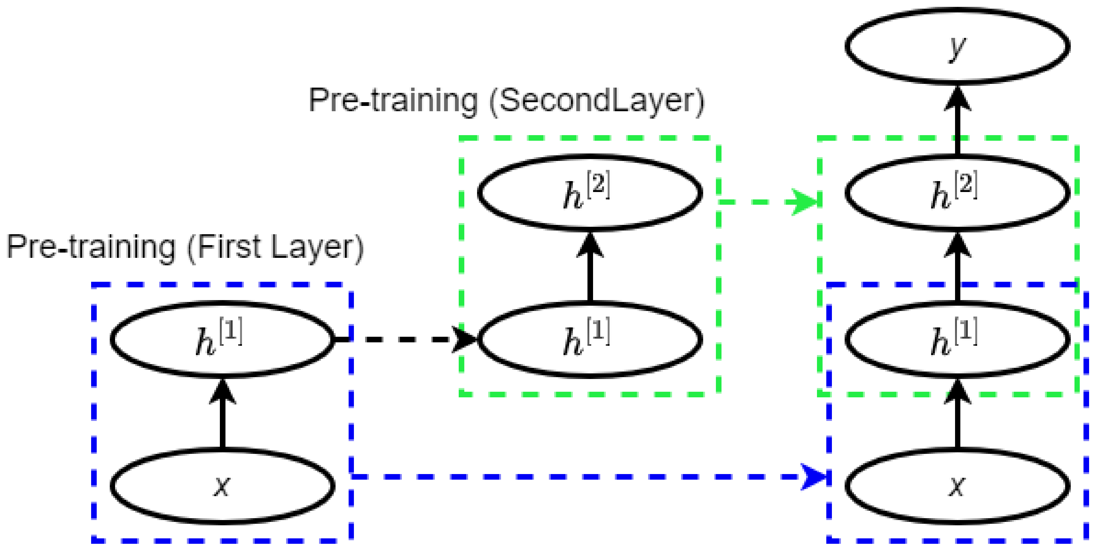
Figure 4.
An architecture of a convolutional neural network (CNN) (adopted from [39]).
Figure 4.
An architecture of a convolutional neural network (CNN) (adopted from [39]).

Figure 5.
A graph convolutional network (GCN) (adopted from [41]).
Figure 5.
A graph convolutional network (GCN) (adopted from [41]).

Figure 6.
Architecture of a generative adversarial network (GAN) (adopted from [42]).
Figure 6.
Architecture of a generative adversarial network (GAN) (adopted from [42]).

Figure 7.
Architecture of an autoencoder (AE) (adopted from [45]).
Figure 7.
Architecture of an autoencoder (AE) (adopted from [45]).
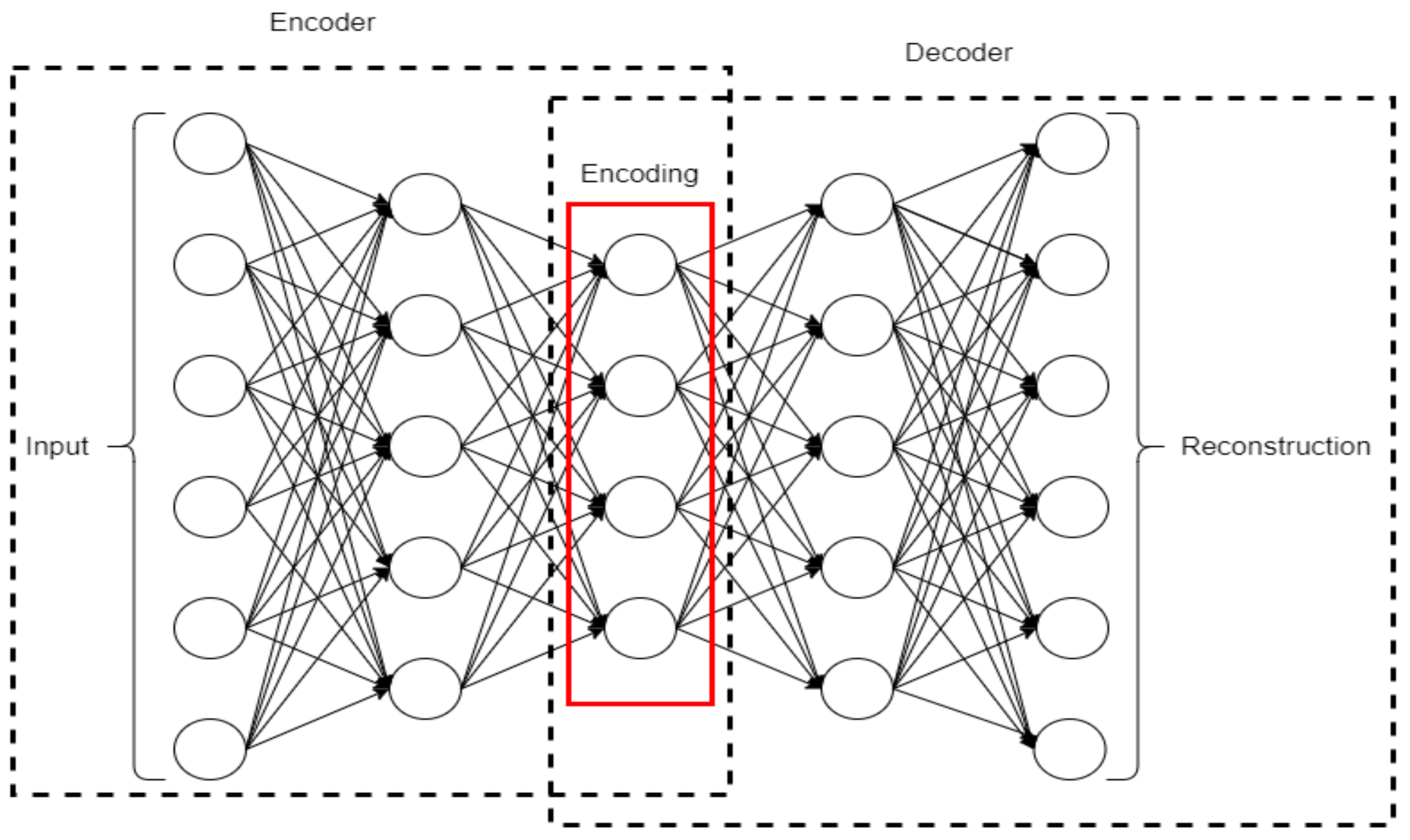
Figure 8.
A simple architecture of an RNN.
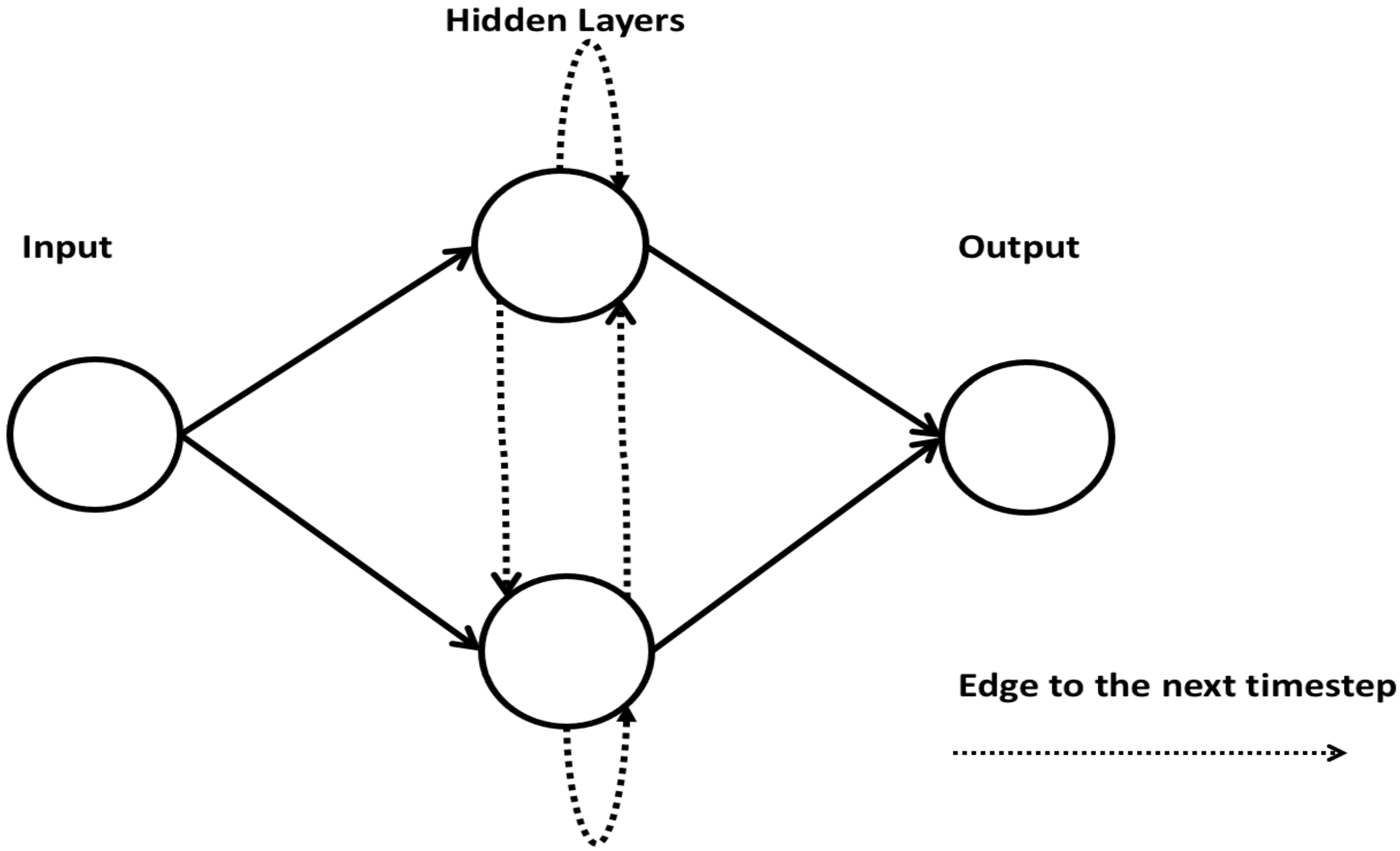
Figure 9.
A long short-term memory (LTSM) architecture (adopted from [49]).
Figure 9.
A long short-term memory (LTSM) architecture (adopted from [49]).

Figure 10.
A bidirectional LSTM (BLTSM) architecture. A and A’ represent an LSTM cell propagating data dependency in forward and reverse directions, respectively. xt and yt are input and output at timestep t from each LSTM cell, respectively. S0 and S’0 denote the initial states, whereas Si and S’i denote the final states.
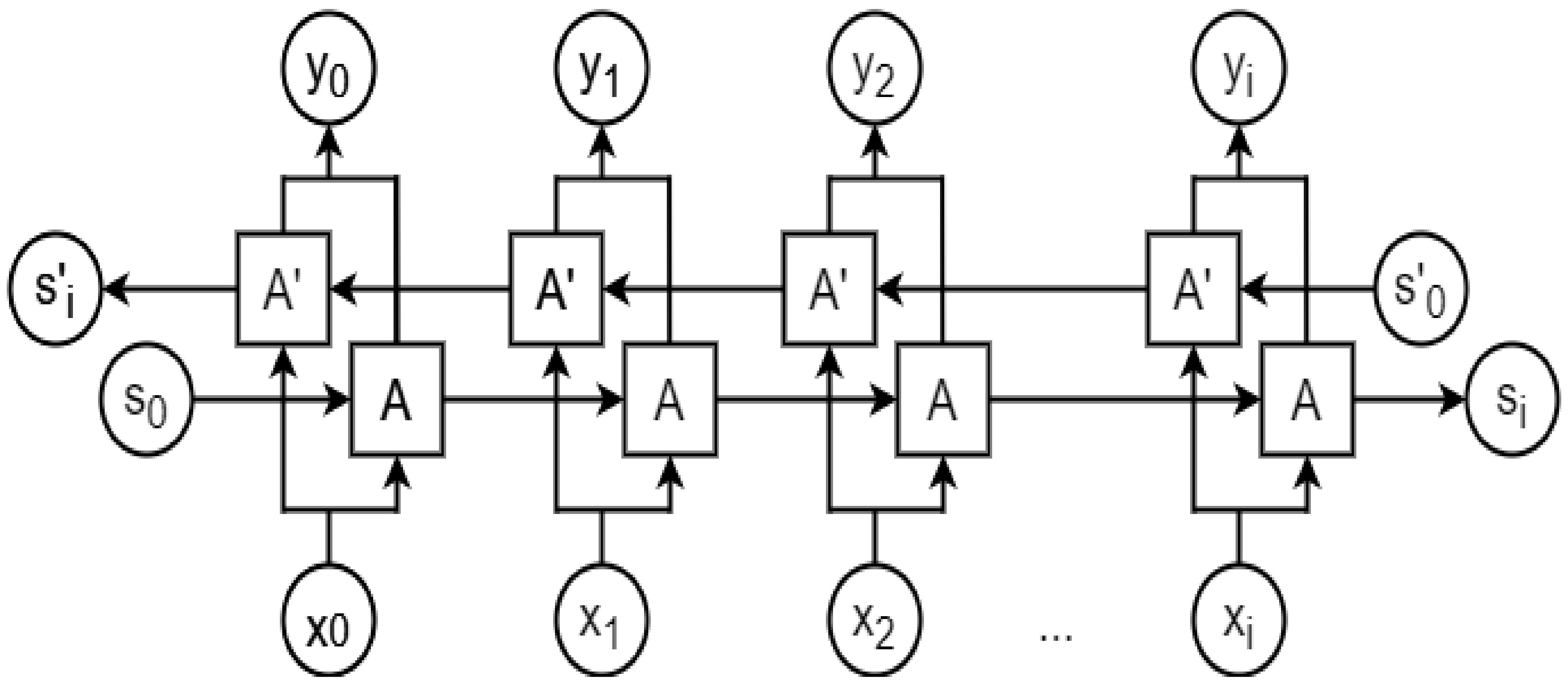
Figure 11.
An attention mechanism (AM) (adopted from [51]). denotes the output map from the middle of the convolution layer of a network. The map is propagated to the next layer of the network, and the AM calculates the weighted average of as . The fully connected layer calculation is represented by the straight lines, and the weighted average calculation is represented by dashed lines. The neural network is utilized by the AM to estimate and the importance of each .

Figure 12.
Loss function and performance metric over epoch to avoid the overfitting problem of deep networks. When the model performance of a validation set diminishes relative to the performance of a training set, an overfitting scenario may be indicated.
Figure 12.
Loss function and performance metric over epoch to avoid the overfitting problem of deep networks. When the model performance of a validation set diminishes relative to the performance of a training set, an overfitting scenario may be indicated.


Table 1.
List of deep learning (DL)-based architectures that have been employed to solve key questions in lncRNA research.
Table 1.
List of deep learning (DL)-based architectures that have been employed to solve key questions in lncRNA research.
| Research Area | Proposed DL Based Architecture | References |
|---|---|---|
| LncRNA Identification | CNN and RNN | LncRNAnet [52] |
| DBN | LncADeep [53] | |
| Embedding vector, BLSTM, CNN | Liu et al. [54] | |
| DNN | DeepLNC [55] | |
| Distinct transcription regulation of lncRNAs | CNN | DeepCNPP [56], DeePEL [57] |
| Functional annotation of lncRNAs | DNN | LncADeep [53] |
| Localization prediction | DNN | DeepLncRNA [58] |
| lncRNA–protein interaction | Stacked auto-encoder, Random forest | IPminer [59], RPI-SAN [60], BGFE [61] |
| Stacked auto-encoder, CNN | RPITER [62] | |
| LncRNA–miRNA interaction | GCN | GCLMI [63] |
| LncRNA–DNA interaction | GCN | [64] |
| LncRNA–disease association | GCN and AM | GCNLDA [65] |
| CNN and AM | CNNLDA [66] | |
| DNN | NNLDA [67] | |
| Cancer type classification | MLP, CNN, LSTM, DAE | [68] |
AM: attention mechanism. BLSTM: bi-directional long short-term memory. CNN: convolutional neural network. DAE: deep autoencoder. DBN: deep belief network. DNN: deep neural network. GCN: graph convolutional network. LSTM: long short-term memory. MLP: multi-layer perceptron. RNN: recursive neural network.
Table 2.
Overview of articles for lncRNA identification leveraging DL-based techniques.
| LncRNAnet [52] | LncADeep [53] | Liu et al. [54] | DeepLNC [55] | |
|---|---|---|---|---|
| Publication Year | 2018 | 2018 | 2019 | 2016 |
| Species | Human and Mouse | Human and Mouse | Human and Mouse | Human |
| Data source used | GENCODE 25, Ensembl | GENCODE 24, Refseq | GENCODE 28, Refseq | LNCipedia 3.1, Refseq |
| Number of lncRNA considered for training | ~21k (~21k) lncRNA transcripts from human (mouse) | ~66k (~42k) full length lncRNA transcripts from human (mouse) | 28k (~17k) lncRNA transcripts from human (mouse) | ~80k lncRNA transcripts and ~100k mRNA transcripts |
| Performance metric | SN, SP, ACC, F1-Score, AUC | SN, SP, Hm | SN, SP, ACC, F1-Score, AUC | SN, SP, ACC, F1-Score, Precision |
| Metrics for comparison against traditional ML based model * | ACC:91.79 # | Hm: 97.7 # | ACC:96.4 # | ACC: 98.07 |
| Intriguing features from the proposed model | ORF length and ratio | ORF length and ratio, k-mer composition and hexamer score, position specific nucleotide frequency etc. | k-mer embedding | Solely based on k-mer patterns |
| Source code/Implementation | N/A | https://github.com/cyang235/LncADeep/ | N/A | http://bioserver.iiita.ac.in/deeplnc |
ACC: accuracy. AUC: area under the receiver operating characteristics curve. Hm: harmonic mean of sensitivity and specificity. MCC: Matthews correlation coefficient. N/A: not available. ORF: open reading frame. SN: sensitivity. SP: specificity. * Performance metrics that were highlighted in the original research article for comparing against traditional machine learning (ML)-based models. #: Performance on humans.
Table 3.
Overview of articles for demystifying transcription regulation of lncRNA leveraging DL-based techniques.
Table 3.
Overview of articles for demystifying transcription regulation of lncRNA leveraging DL-based techniques.
| DeepCNPP [56] | DeePEL [57] | |
|---|---|---|
| Publication Year | 2019 | 2019 |
| Species | Human | Human |
| Data source used | Dataset from [75] | FANTOM CAT [17] |
| Number of lncRNA transcripts or genes considered | ~19k lncRNA genes | ~7k (~3k) p-lncRNA (e-lncRNA) transcripts |
| Performance metric | SN, SP, ACC | SN, SP, MCC, AUC |
| Metrics for comparison against traditional ML based model * | ACC: 83.34 | Traditional ML model does not exist for this task |
| Intriguing features from the proposed model | k-mer embedding of promoter regions | k-mer embedding of promoter regions, transcription factor binding sites |
* Performance metrics that were highlighted in the original research article for comparing against traditional ML-based models.
Table 4.
Overview of articles for lncRNA–protein interaction prediction leveraging DL-based techniques.
Table 4.
Overview of articles for lncRNA–protein interaction prediction leveraging DL-based techniques.
| IPminer [59] | RPI-SAN [60] | BGFE [61] | RPITER [62] | |
|---|---|---|---|---|
| Publication Year | 2016 | 2018 | 2019 | 2019 |
| Species | Multi-species | Multi-species | Multi-species | Multi-species |
| Benchmark Data source used | NPInter 2.0, RPI369, RPI488, RPI1807, RPI2241, RPI13254 | NPInter 2.0, RPI488, RPI1807, RPI2241 | RPI488, RPI1807, RPI2241 | NPInter 2.0, RPI369, RPI488, RPI1807, RPI2241 |
| Performance metric | SN, SP, ACC, Precision, AUC, MCC | SN, SP, ACC, Precision, AUC, MCC | SN, SP, ACC, Precision, AUC, MCC | SN, SP, ACC, Precision, AUC, MCC |
| Metrics for comparison against traditional ML based model for different dataset * | NPInter 2.0 (ACC: 95.7) #, RPI369 (ACC: 75.2), RPI488 (ACC: 89.1), RPI1807 (ACC: 98.6), RPI2241 (ACC: 82.4), RPI13254 (ACC: 94.5) | NPInter 2.0 (ACC: 99.33) #, RPI488 (ACC: 89.7), RPI1807 (ACC: 96.1), RPI2241 (ACC: 90.77) | RPI488 (ACC: 88.68), RPI1807 (ACC: 96.0), RPI2241 (ACC: 91.30) | NPInter 2.0 (ACC: 95.5) #, RPI369 (ACC: 72.8), RPI488 (ACC: 89.3), RPI1807 (ACC: 96.8), RPI2241 (ACC: 89.0) |
| Intriguing features from the proposed model | Sequence composition features, specifically 3-mer and 4-mer from protein and RNA sequences, respectively | k-mer sparse matrix from RNA sequences and PSSM from protein sequences | k-mer sparse matrix from RNA sequences and PSSM from protein sequences. Stacked auto-encoder was employed to get high accuracy | k-mer frequency of sequence and two types of structural information (bracket and dot) from RNA. k-mer frequency of sequence and three types of structural information (α-helix, β-sheet and coil) from protein |
| Source code/Implementation | https://github.com/xypan1232/IPMiner; http://www.csbio.sjtu.edu.cn/bioinf/IPMiner | N/A | N/A | https://github.com/Pengeace/RPITER |
PSSM: position-specific scoring matrix.* Performance metrics that were highlighted in the original research article for comparing against traditional machine learning (ML)-based models. #: Performance on humans.
Table 5.
Overview of articles for lncRNA–disease association prediction leveraging DL-based techniques.
Table 5.
Overview of articles for lncRNA–disease association prediction leveraging DL-based techniques.
| GCNLDA [65] | CNNLDA [66] | NNLDA [67] | |
|---|---|---|---|
| Publication Year | 2019 | 2019 | 2019 |
| Data source used | LncRNADisease, Lnc2cancer, GeneRIF | LncRNADisease, Lnc2cancer, GeneRIF | LncRNADisease |
| Number of lncRNA considered | 240 | 240 | 19166 |
| Number of diseases considered | 402 | 402 | 529 |
| Performance metric | AUC, AUPRC, Precision, Recall | AUC, AUPRC, Precision, Recall | HR(k): Probability for the predicted samples to appear in top-k ranked list |
| Metrics for comparison against traditional ML based models | AUC $: 0.959 AUPRC $: 0.223 | AUC $: 0.952 AUPRC $: 0.251 | HR(k); k = 1.10 |
| Intriguing features from the proposed model * | For ncRNA-lncRNA similarity Chen’s method was applied [105]. For disease-disease similarity Wang’s method was applied [106] | For ncRNA-lncRNA similarity Chen’s method was applied [105]. For disease-disease similarity Wang’s method was applied [106] | Matrix factorization method was modified in two aspects to fit into this model: (a) cross-entropy was used as a loss function; (b) only one batch data per round was used to minimize loss |
| Source code/Implementation | N/A | N/A | https://github.com/gao793583308/NNLDA |
AUPRC: area under the precision-recall curve. HR(k): hit ratio, the probability for the predicted samples to appear in a top k ranked list. * Performance metrics that were highlighted in the original research article for comparing against traditional ML -based models. $: Average over 402 diseases.
Publisher’s Note: MDPI stays neutral with regard to jurisdictional claims in published maps and institutional affiliations. |
© 2020 by the authors. Licensee MDPI, Basel, Switzerland. This article is an open access article distributed under the terms and conditions of the Creative Commons Attribution (CC BY) license (http://creativecommons.org/licenses/by/4.0/).
Share and Cite
MDPI and ACS Style
Alam, T.; Al-Absi, H.R.H.; Schmeier, S. Deep Learning in LncRNAome: Contribution, Challenges, and Perspectives. Non-Coding RNA 2020, 6, 47. https://0-doi-org.brum.beds.ac.uk/10.3390/ncrna6040047
AMA Style
Alam T, Al-Absi HRH, Schmeier S. Deep Learning in LncRNAome: Contribution, Challenges, and Perspectives. Non-Coding RNA. 2020; 6(4):47. https://0-doi-org.brum.beds.ac.uk/10.3390/ncrna6040047
Chicago/Turabian StyleAlam, Tanvir, Hamada R. H. Al-Absi, and Sebastian Schmeier. 2020. "Deep Learning in LncRNAome: Contribution, Challenges, and Perspectives" Non-Coding RNA 6, no. 4: 47. https://0-doi-org.brum.beds.ac.uk/10.3390/ncrna6040047
Note that from the first issue of 2016, this journal uses article numbers instead of page numbers. See further details here.