Article

Analyzing the Raman Spectra of Graphenic Carbon Materials from Kerogens to Nanotubes: What Type of Information Can Be Extracted from Defect Bands?

1
CEMES, UPR8011-CNRS, Université de Toulouse, 29 rue Jeanne Marvig, 31055 Toulouse CEDEX 04, France
2
Nanoscience Research Laboratory, Pontificia Universidad Católica Madre y Maestra, Autopista Duarte km 1 ½, Apartado Postal 822, Santiago, Dominican Republic
3
IMT Mines Albi, Centre RAPSODEE, UMR CNRS 5302, Campus Jarlard, F-81013 Albi CEDEX 09, France
4
Institute of Nano Science and Technology, Habitat Center, Sector 64, Phase 10, Mohali, Punjab 160062, India
5
CNRS/MIT/Aix-Marseille Université Joint Laboratory “MultiScale Materials Science for Energy and Environment”, UMI 2, Massachusetts Institute of Technology, 77 Massachusetts Avenue, Cambridge, MA 02139, USA
*
Author to whom correspondence should be addressed.
Submission received: 30 September 2019 / Revised: 27 October 2019 / Accepted: 30 October 2019 / Published: 1 November 2019
(This article belongs to the Special Issue Characterization of Disorder in Carbons)

Abstract

:
Considering typical spectra of a broad range of carbonaceous materials from gas-shale to nanotubes, various ways by which defects show up in Raman spectra are exampled and discussed. The position, resonance behavior, and linewidth of both the D and G bands are compared, even if in some cases obtaining accurate information on the materials from the fitting parameters is a difficult task. As a matter of fact, even if a full picture is unreachable, defining parameter trends is one acceptable option. Two ways to determine the linewidth, either graphically and or by fitting are proposed in order to be able to compare literature data. The relationship between the crystallite size obtained from the linewidth and from X-ray diffraction, which is complementary to the Tuinstra and Koenig law, is examined. We show that a single approach is not possible unless modeling is performed and therefore that analysis of Raman spectra should be adapted to the specificities of each sample series, i.e., a minimum of knowledge about the materials is always required.

Graphical Abstract

1. Introduction

Raman spectroscopy is widely used for investigating carbonaceous materials [1,2,3,4]. The Raman signal is intense enough to map samples and the shape of the spectra presents modifications with respect to the chemical composition or crystallite size [5,6]. For example, Raman spectroscopy has become a routine technique for the analysis of graphene, allowing the charge transfer, layer quality, or number of layers to be obtained [7]. The Raman signal of all carbon allotropes is well known [8]. However, analyzing Raman spectra becomes more complex as the crystallite size becomes smaller. Considering point defects (e.g., vacancies, bonded atoms or functional groups) in small graphene domains has led to new models [9] for which discriminating point defects from domain edges (line defects) have been recently proposed [10]. It is presently a real concern for physicists to propose models and to try to accurately extract physical parameters from Raman spectra. For a long time, the Tuinstra and Koenig law [11] was believed to relate with no restriction the crystallite size to the ratio of Raman intensity height ID/IG, where D is the defect band (around 1330 cm−1) and G is the optical phonon of carbon atoms moving in phase opposition around (1580 cm−1). Nowadays, it is clear that the Tuinstra and Koenig law is suitable for some particular samples only. Indeed, in many carbon materials, heteroatoms are present in a sufficient amount to significantly modify the Raman spectra. In a recent paper dealing with the contribution of both point and line defects to the Raman signal [10], the EL4 dependence (where EL is the excitation laser energy) of the ID/IG ratio found for graphite [12] was assumed. However, this hypothesis has been invalidated by experiments on small crystallite sizes [13]. Usually, crystallite size is determined by X-ray diffraction. Determining crystallite size by Raman spectroscopy is highly expected as the process can be local with a spatial resolution in the micrometer range and there is no need for any sample preparation. For disordered carbons (i.e., with La in the range of 2 nanometers and below) fitting the Raman spectra is definitely an issue because there is no consensus on the way to do it. Even after annealing in the 1000–2400°C range, the fitting is not straightforward and many inaccuracies are often present. Many strategies exist, such as varying the number of sub-bands required for the fitting, and each of them gives different results. Some parameters are commonly used while others such as the D band linewidth are user-dependent and therefore are less investigated. As this band is due to a double resonance process [14] and its linewidth is correlated to the crystallite size [12], using it is highly interesting but requires an accurate understanding of the physical processes which are responsible for it.
In this paper, Raman spectra of disordered carbon materials with increasing La are analyzed first. Then, two particular Raman bands (D and D’) due to a double resonance effect are investigated to show what complementary information can be extracted with ordered carbon materials. Afterwards, how linewidths and intensities vary with crystallite size is summarized and the possible requirements for building a theory able to reproduce experimental Raman spectra are discussed.

2. Experimental Section

2.1. Samples

Carbonaceous materials were deliberately selected from very different origins.
The gas-shale samples used were Mississippian Barnett shale, Fort Worth Basin (Texas, USA) and Marcellus49 shale from Pennsylvania. They were merely cut and not polished. They were studied as they were, i.e., the kerogen part (i.e., the carbonaceous part) was not extracted from the mineral.
The N330 sample used was a commercial carbon black (from Orion Engineered Carbons®) composed essentially of elemental carbon and typically used as a reinforcing filler in tire tread compounds. This grade was produced by the furnace process through the incomplete or partial combustion of a hydrocarbon feedstock. For the purposes of other studies concerned with tire recycling, a model tire containing the N330 carbon black (31.91 wt.%) was first formulated and then thermally treated under two sets of conditions in order to recover the carbon black filler. The first set of conditions (pyrolysis) corresponded to a temperature of 475 °C for 45 min under N2 (flow rate of 5 L/min) at atmospheric pressure. The second set of conditions (steam-thermolysis) corresponded to the very same cycle but under water vapor instead of N2 (flow rate of 5 L/min).
Cokes at various carbonization temperatures were prepared from a coal tar pitch (reference GFEC-1) by Le Carbone Lorraine (now MERSEN) and obtained from the French Carbon Society (SFEC, formerly GFEC) to be used as reference samples.
Carbon cones were grown by chemical vapor deposition from the thermal cracking above 1300 °C of a CH4 and H2 mixture onto single carbon nanotubes [15]. The first step involved catalytically growing individual multiwall carbon nanotubes and then, during a post-growth catalyst-free process, adjusting experimental conditions to deposit pyrolytic carbon onto the nanotube and form the cones.
Single-wall carbon nanotubes (SWCNT) were grown horizontally aligned on a substrate of stable temperature (ST)-cut quartz with patterned lines of iron catalyst spaced by 400 µm. Ethanol vapor was used as a carbon precursor and was diluted in argon. The growth was performed at a temperature of 850 °C for 30 min. The occurrence of nanotubes was deliberately low so that the tubes were individual on the surface. Under the selected experimental conditions, the nanotube diameters were in the 1.1 nm to 1.5 nm range.

2.2. Experimental Conditions

A UV-Dilor spectrometer was used in a backscattering configuration with an excitation wavelength of 336 nm (3.69 eV). The laser power was kept low enough (5 mW with a ×20 objective) to avoid modifying the materials by overheating. For the visible range, both an XPlora and a Labram HORIBA Jobin-Yvon spectrometer provided by HORIBA France, Longjumeau, France were used. These were bright enough to allow using a laser power below 1 mW with a ×40 objective while obtaining a recordable signal with a reasonable noise level. A wavelength of 532 nm (2.33 eV) was usually used. The Labram spectrometer was coupled to a Trios atomic force microscopy (AFM), allowing for the possibility of characterizing the cone apex with a nanometric resolution and also to acquire a tip-enhanced Raman spectrometer (TERS) signal using commercial silver tips working at 633 nm.
The X-ray diffraction (XRD) experimental diagrams were recorded on a Bruker D8 Advance diffractometer equipped with a Cu anode source and a Lynxeye 1D detector using a Bragg-Brentano setup. The primary divergence slit aperture was fixed at 0.5°. The XRD diagrams were recorded in a 2θ range between 10° and 90° with a 0.01° step in continuous mode.

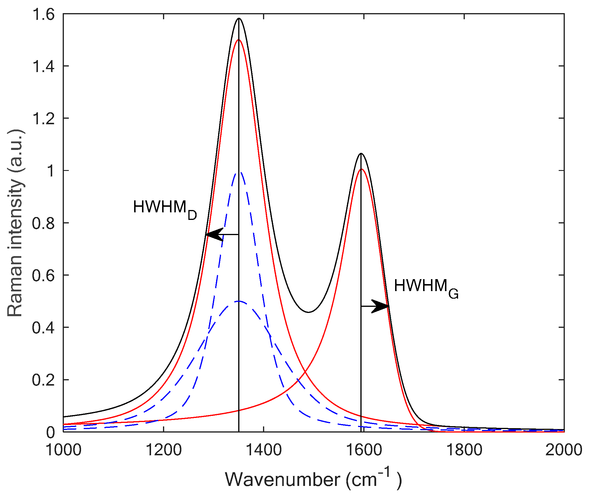
2.3. Fitting Procedure

Fitting the Raman spectra can be done with 10 [16], 5 [6], or fewer than 5 sub-bands [17]. Ferrari and Robertson [1,3,4] as well as Fung et al. [18] have used a Fano shape for fitting both the G and D bands with success. When the number of functions used is larger than two, the fitting becomes excellent but each parameter is highly sensitive to small shape changes.
For poorly organized carbon materials such as kerogens, considering up to five bands to account for the D and G spectral region (sometimes the spectral positions are fixed in order to have the same, single decomposition for all the samples) allows for having a kind of spectral decomposition close to principal component analysis. This is an interesting way to compare small shape variations within a series of samples. Nevertheless, in such an approach, the linewidth of both the D and G bands (or bands close to the related spectral positions and called by these names) are underestimated and cannot be properly compared.
Alternatively, as long as the D band position is sensitive to the excitation energy and the signal around the D band varies in the same way, a double Lorentzian centered on a single position may be proposed to fit the D band of graphenic materials. This double Lorentzian can fully take into account for both the double resonance process and a possible double scattering event [13]. This principle applies to all kinds of graphenic carbons whatever their level of structuration, although in practice the possible double scattering process cannot occur anymore for La > ~5 nm, meaning the related Lorentzian vanishes and hence that considering a single Lorentzian is enough for larger La.
Due to the large variety of Raman spectrum shapes, the Lorentzian shape has been viewed as too restrictive and switching to a Voigt shape (a mixing of Lorentzian and Gaussian shapes) definitively better. In the following, in order to compare all the spectra from all the samples from our series, the D band is fitted with a double Voigt band (Figure 1) as an adaptation of the procedure proposed in [13]. For simplicity, we only report the resulting D band curve. For the G band, the Fano shape is suitable for taking into account the low wavenumber range but is usually associated with a small lack of intensity in the upper side of the band. This is unsatisfactory and consequently using a Fano shape for the low wavenumber side of the band and a Voigt shape for the upper side is proposed here. The switch from one shape to the other is chosen to be at the maximum of the curve, corresponding to the G band wavenumber.
The main problem of fitting arises with amorphous carbon where the spectra present a single band with a strong asymmetry and are consequently very difficult to describe. In this paper, we have not considered amorphous carbon materials in which graphenic character is not prevalent anyway and therefore barely compare to the graphene-based carbons of the series investigated.
Graphically, it is possible to extract some parameters from direct measurements of the Raman spectra. Considering a linear background, the intensity height of both the D and G bands (ID and IG) can be directly measured with a ruler. This has been used in the past and also in review work to compare data [19]. For the linewidth, it is important to specify whether it is half (HWHM) or full (FWHM) width at half maximum as both are used in the literature. HWHM can be also measured using a ruler as indicated in Figure 1.
The ratio of ID/IG depends on the excitation energy EL and we note α the exponent in the expression
I D I G = f ( L a ) E L α
where f(La) is a function of the in-plane crystallite size La.

2.4. La, Lc, and LD Parameters and Experimental Laws in the Literature

Carbon materials are composed of domains, or crystallites, which may be defined as the smallest coherent volumes of matter. It is remarkable that, for a given precursor and a given carbonization temperature, the distribution of domain sizes is relatively narrow and can be well represented by its average value, as obtained by XRD measurements. XRD is usually used to determine two parameters, the height Lc of the average domain along the c axis (even if the stacking is random) and determined from the 002 peak width, and the average diameter La of the graphene planes composing the domain, deduced from 10 (when the stacking sequence is turbostratic) or 100 (when the stacking sequence is at least partly graphitic) [20].
In the first publication of Tuinstra and Koenig [11], using both blue and green excitation wavelengths, a correlation was found with the Raman spectrum data, i.e.,
I D I G = 4.4 L a ( n m )
where I is the height of the Raman D and G bands. A can be used instead of I when areas are preferably considered over intensities. Indeed, as graphene became a worldwide subject of study, the question of whether either the area of a peak or its height should be used to describe the Raman response was considered. Unfortunately, a misunderstanding of the factor relating the XRD peak linewidth and crystallite size has led to inaccurate laws (see the discussions in references [13] and [21]). Moreover, the dependence of ID/IG on the excitation energy was assumed to be EL−4, whereas this factor was found to be only valid for a limited crystallite size range [13]. Finally, the following relation proposed in [22] has often been considered as a reference since then:
L a ( n m ) = 560 E L 4 1 A D A G
In their text, however, the authors use the term “relative intensity” when designating integrated area and write it improperly as I (we have corrected the notation in Equation (3)).
When considering the D band, when graphenes are affected by point defects (as created by ion bombardment, for instance) only, the situation is simple as the following law has been proposed versus the excitation energy for LD (the average distance between defects) > ~7 nm [9], i.e.,
L D ( n m ) = 3640 E L 4 1 A D A G
For LD < ~7 nm (see below), a more complex expression has been proposed, taking into account two spatial areas, namely a defective one and another one where the D band is activated. In such a relation (Equation (4)), the EL2 dependency for the determination of LD of around 2 nm (and of course lower) does not perfectly fit with the experimental data.
Finally, by combining all experimental laws, the discriminating contributions of point and line defects in the Raman spectra of graphene-related materials have been proposed [10] while omitting the limitation due to the modification of the EL4 dependency.
For highly disordered graphenic carbons (La < 2 nm), the situation is different. Ferrari and Robertson proposed a variation in La2. This led to the well-known reference plot [1] showing an increase in La2, a maximum around La = 2 nm, and a decrease following the Tuinstra and Koenig law. This is obviously consistent with their previous publications on amorphous carbon (both pristine and annealed at moderate temperature, i.e., below 500 °C).
Equations (3) and (4) have been obtained for nano-graphite and graphene. In many other samples, the presence of heteroatoms modifies the shape of the D band and introduces some wavenumber shift, and consequently only parameter trends can be proposed [2,3,4].
This is typically true for geological samples for which the decomposition in several bands is often used in order to reveal some correlation between the samples and then to determine from it their age or the temperature ultimately reached during a geologic cycle [23]. For chars, the same strategy with several bands is used [24], with, however, variable success. Some particular spectra resist this approach as they are too sensitive to initialization parameters and correspond to many different fitting solutions. Due to these difficulties, for example for soot, spectrum subtraction without fitting has been proposed [25].
The linewidth has been also intensively used [19] for determining La for a large range of graphenic carbons. From the confinement model, HWHM is related to the crystallite size by [26]:
H W H M D ( c m 1 ) 300 L a ( n m )
The value 300 includes the slope dωD/dEL, where ωD is the wavenumber of the D peak. This expression is satisfactory for many samples for La larger than 2–3 nm.
The data analysis and related discussion that follow attempt to bring some clarity to this fuzzy situation.

3. Experiments on Poorly Ordered Graphenic Carbon Materials

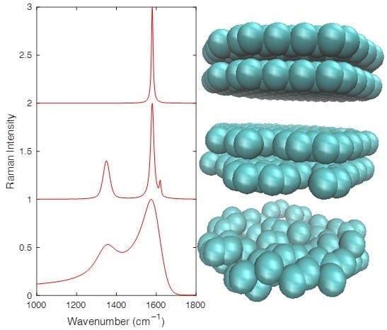
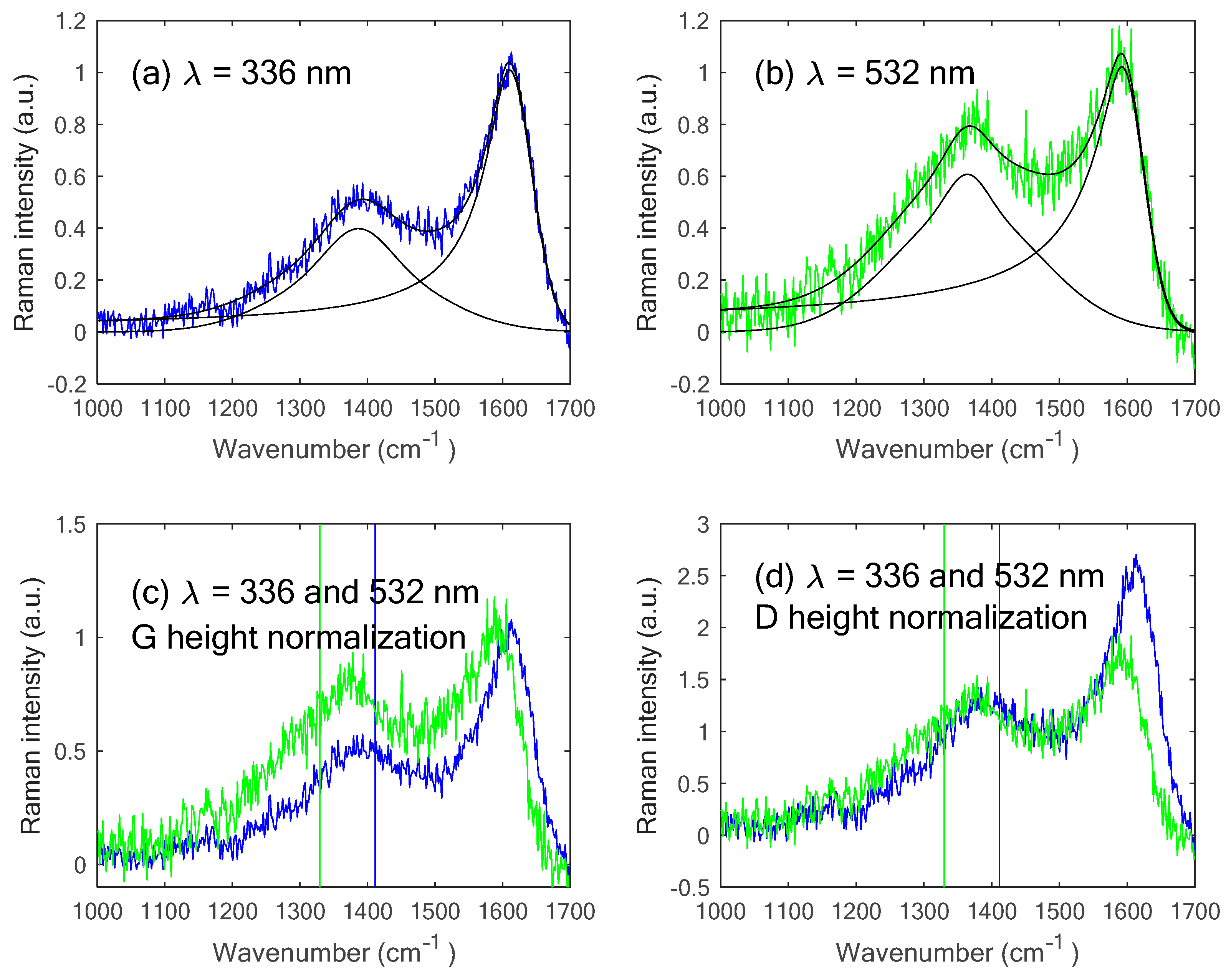
3.1. Crystallite Size Lower Than 2 nm − The Example of Gas-Shales

Two gas-shale samples with different maturities are compared here. The Barnett sample contains both oil and gas while the Marcellus49 sample contains only gas (hydrocarbons), meaning that its maturity is higher (assuming that no incoming or outgoing fluid migration events have occurred either for gas or oil). In Figure 2 and Figure 3 are reported the Raman spectra for both samples obtained with an excitation wavelength of 336 nm (a) and 533 nm (b), respectively. The fitting with two bands as described in Section 2.3 is fairly satisfactory. It is noteworthy that in the following we name the two main bands as D and G in order to be consistent with the literature; these denominations, however, are questionable for such materials (see below).
In order to clearly see the differences between the spectra and understand the strategies used in the literature, the spectra are normalized to either the intensity of the G band or of the D band ((c) and (d), respectively, in both figures). The fitting parameters are reported in Table 1.
Studying poorly organized carbonaceous materials such as gas-shale samples allows for the investigating further of the behavior of the D and G bands. The linewidth is not a good indicator (because the crystallite size is small and the Raman behavior is close to a molecular response) and neither is the position. First of all, the D band intensity is weak and poorly sensitive to the excitation wavelength. This is related to the high heteroatom content associated with the carbon lattice. Indeed, for pure yet defective graphenic materials, no D band shows up with UV excitation. Also, the shift of the D band wavenumber with the excitation energy for graphite is around 60 cm−1/eV [14], while here, the shift value is much smaller (Table 3, column 8). These two features are enough to figure out that the band which shows up in the 1300–1400 cm−1 range is not the genuine D-band that carbon scientists are used to. The double resonance effect vanishes (as well as the double scattering effect) and the D band, in this case, is close to corresponding to the breathing of a single hexagonal ring of carbons [1]. Even if the intensity ratio of the D band over the G band increases when the excitation energy is reduced, the behavior resonance does not follow the EL4 dependency. Hence, only qualitative information can be obtained.
Several fitting strategies exist for kerogens and each of them is valid for a given sample series for obtaining variations of some parameters. However, none is universally valid (see Section 2.3). The physical meaning of fitting with two bands only is not obvious. The linewidth of the D band is no longer exclusively governed by the double resonance process and consequently the correlation between the linewidth and the crystallite size is no longer valid (one can note that the slope dωD/dEL is reduced and consequently that the HWHM of the D band is reduced too). We have also normalized to either the D or G band intensity in order to visually compare the results. The conclusion is that for the oil kerogen (Barnett), normalizing to the D band intensity is more relevant as both the G band shape and position change a lot. For the gas kerogen sample (Marcellus49), normalizing to the G band appears to be better.
One can note that fitting the D band with a symmetrical function brings to light the peak at 1265 cm−1 for the Marcellus sample. This band can originate from two causes: (i) the activation of phonon density of states around the K point (for transverse optical (TO) branches) due to a double resonance process, and (ii) another organic phase in the sample. Indeed, recently, a band located at 1450 cm−1 has been tentatively attributed to the presence of trapped liquid hydrocarbons [27]. As this 1450 cm−1 value does not correspond to a particular point in the phonon band dispersion nor in the phonon density of states of graphite, this assignment is not challenged by the double resonance theory.
In summary, the Barnett sample presents a D band which is poorly sensitive to excitation energy, revealing a lack of large graphitic domains, and a G band for which high sensitivity to excitation energy is due to a large amount of hydrogen in interaction with the graphenic lattice (aromatic C–H). [2] Comparatively, the Marcellus49 sample is more mature, with less hydrogen in the lattice (its G band is less sensitive to excitation energy than that of Barnett), and exhibits larger domains (the wavenumber of its D band is more sensitive to excitation energy). The results are thus consistent with the maturity trend presumably assumed, confirming the higher rank for Marcellus49 and providing a good hint that no migration event has affected the oil and/or gas content for both shales.

3.2. Crystallite Size Directly Above 2 nm: The Example of Carbon Black

This sample series contains three samples: the original commercial carbon black N330, then the same after incorporation within a model tire, and subsequently the same which has been subjected to either pyrolysis or steam-thermolysis (see Section 2.1).
In Figure 4 are reported the diffractograms for the three samples. In a previous work [20] we developed an accurate fitting procedure from a bottom-up approach, allowing the average in-plane crystallite size La to be the only adjustable parameter.
Judging from the XRD data, the carbon blacks are definitely not exactly the same before and after heat treatment. The other peaks in the diffractogramm are due to crystalline compounds incorporated as vulcanisation agents into the model tyre formulation. For the original N330 La ~2.9 nm while it is 2.4–2.5 nm for the recovered carbon blacks. The difference is significant. The most probable origin is the surface functionalisation of the crystallite by the elastomer functional groups while being decomposed. Lc can be seen to have increased after the post-treatments. This value takes into account the correction necessary for small crystallite size [20]. At a constant number of carbon atoms, Dopita et al. [28] have shown that the shape of the crystallite does not play a role in the linewidth of 002. It is believed that this is due to the contribution of the carbonised remnants of the elastomer which were not fully eliminated by the treatments and ended by coating the carbon black nanoparticles, thereby adding atoms to the crystallite and so leading to an increase in Lc [28].
In order to analyse further the differences, two Raman spectra at 532 nm (2.33 eV) and 638 nm (1.96 eV) were acquired for each sample (Figure 5). Spectra were fitted and the extracted parameters are reported in Table 2.
What is striking is the change in the resonance behavior of the ratio ID/IG. The power dependence deduced from these two excitation wavelengths is completely different, and we assume that the amount of hydrogen plays a role like that in luminescence [29]. In any case, this means that extracting accurately the crystallite size from ID/IG is not possible. Indeed, even if it seems correct at the excitation energy of 2.33 eV, the Raman spectra at 1.96 eV are too different. Another option is then to use the linewidth. Comparing the linewidth of the G bands, we clearly see that the increase of it versus the decreasing crystallite size is no longer valid. We have proposed a law in a previous work [13] but it is clear that this increase is only valid over a small range (typically between 2–3 to 10 nm).
It therefore remains to consider the linewidth of the D band. For both excitation wavelengths the expected trend is observed and from the law obtained with the confinement model (La ≅ 3600/HWHMD), at 532 nm (most Raman works are done in the green), crystallite sizes of 2.1, 2.3, and 2.5 nm for steam-thermolysis, pyrolysis, and the reference sample were obtained, respectively. However, compared to the X-ray data, this is not consistent. Moreover, the shift of the D band versus the excitation energy (column 8 in Table 2) is not consistent either, proving that the Raman response of the carbon domain is affected by the recycling process.
As the main conclusion from the study of both the carbon black series and the previous shale series, it appears that the Raman response is highly sensitive to the amount of heteroatoms, which modify the electronic band structure. Therefore, would the average crystallite sizes for a pure graphenic carbon and a heteroatom-rich carbon be the same, the Raman response might be different, hence preventing an accurate comparison between both. This explains why, in the literature, decompositions in several sub-bands are used and correlations are sought to estimate the chemical composition but that they will always fail in the determination of the crystallite size. The use of several indicators (e.g., linewidth of both D and G bands as well as the ratio ID/IG) improves the comparison between samples.

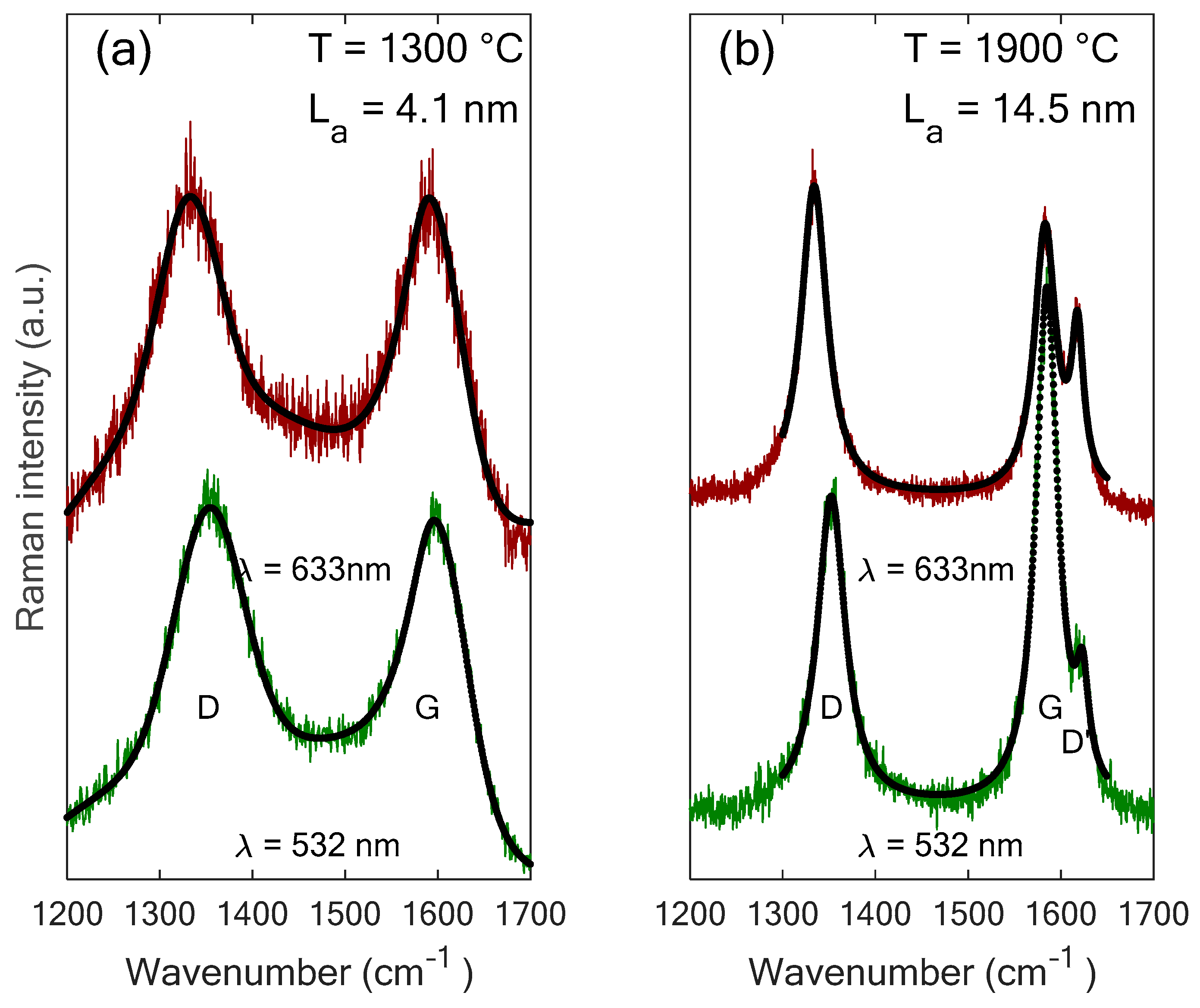
3.3. La Much Larger Than 2 nm: The Example of Coal Tar Pitch Cokes

Another Raman band which somehow accounts for defects is the D’ band. This band does not show up in poorly organised carbons such as the kerogens and carbon black investigated in Section 3.1 and Section 3.2, and hence we considered other carbon materials. A complete set of XRD data on the coal tar pitch coke series considered here can be found in [20]. Only Raman spectra are reported here (Figure 6) for two excitation wavelengths (532 and 633 nm, respectively) and for two coke samples (carbonised at 1300 and 1900 °C, respectively, so that they exhibit different crystallite sizes).
When the crystallite size is large, the D’ band is clearly visible (and highly sensitive to an excitation energy with 1/EL4 dependency of ID or ID’ over IG). When the crystallite size is lower than 7 nm [13], both G and D’ merge into a single band [18,30]. The shape of this merged band is nearly insensitive to the excitation energy and the linewidth remains constant over a large range of excitation energies, at least from 2 to 4 eV. The resonance behavior of the ID/IG ratio is also modified: with large crystallite sizes, it follows the law 1/EL4, whereas the exponent 4 is reduced to a lower value (always positive) for small crystallite sizes. By comparing the spectrum at 633 nm and that at 532 nm for the 1900 °C coke in Figure 6 (right), it is obvious that the ID/IG ratio is remarkably different for both wavelengths while it remains quite similar for the 1300 °C coke. Therefore, the ID/IG ratio behaves differently for both samples due to the occurrence of the D’ band. Equation (2) could be associated with La < ~7 nm and Equation (3) with La > ~7 nm.

4. Experiments on Highly Ordered Graphenic Carbon Materials

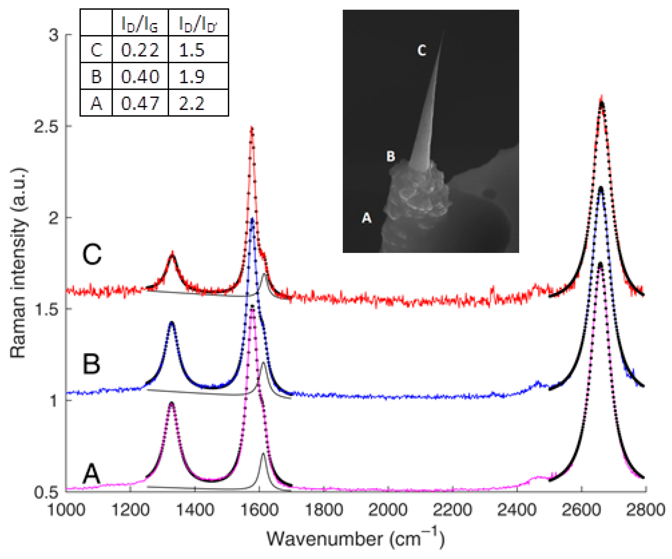
4.1. Fewly Defective, Turbostratically Stacked Graphenes – The Example of Carbon Cones

For large crystallite sizes, different information can be obtained. For example, the ratio ID/ID’ can be determined. Eckmann et al. [31] have shown that this ratio allows for discrimination between various dominating types of defects. However, one defect is not considered in [31]: the case of loops, which form when two superimposed graphene edges bend, join, and buckle. Such a buckling effect has been commonly observed in the literature, starting as early as in 1981 with heat-treating herringbone carbon nanotubes [32]. The material we have considered which exhibit this kind of loop are carbon nano-cones prepared in our laboratory (see Section 2.1). The whole cone is made of perfect graphenes concentrically displayed and attached to a carbon microfiber segment [33]. Therefore, the cone surface is made of steps, with each step corresponding to a free graphene edge and having the height of a single graphene. When it comes to the cone apex, the nano-size of it generate high stresses (as in small diameter nanotubes), and when superimposed graphenes have their edges close to each other, the carbon atoms from both graphenes bond to each other in order to lower the energy of the system by eliminating the dangling bonds (Figure 7).
When mounting such a carbon cone onto a cantilever and using it as a tip for a TERS system instead of the standard Ag tip, the laser spot can be moved along the cone from A (the carbon microfiber segment) to C (the cone apex) as reported in Figure 8, thanks to the ability of the equipment to focus the laser very accurately in the three space directions.
The associated Raman spectra obtained are also reported in Figure 8. The ID/IG ratio is the highest (0.47) on the microfiber part (A) in which the structural organization is less than in the cone [33] and is the lowest (0.22) on the cone apex (C) where the graphenes are mostly perfect.
Interestingly, the ID/ID’ ratio does not remain constant when moving from A to C, meaning that the type of defect is locally not the same. In A, defects are in part those associated with graphene stacks with small La [33], providing an ID/ID’ ratio of 2.2. On the other hand, at the cone apex, we know from the HRTEM images that the main defect is the loop configuration terminating the graphene edges. Consequently, we associate the quite unusual value (1.5) of the ID/ID’ ratio to this type of defect, thereby completing the table given in the paper of Eckmann et al. [31] (Table 3).
For mounting the carbon cone onto the cantilever, we compared three different assembly processes: firstly, gluing the cone with a single component UV-curable resin at room temperature, secondly, metal (platinum) deposition using focused electrons to break the organometallic precursor molecules, and lastly, the same as the latter but using focused ions instead of electrons. The Raman spectra allow for comparison of the effect of these processes on the cone’s structural integrity (Figure 9).
With respect to the glued cone, which can be taken as the reference material since the operating procedure was not harmful to the graphene lattice (carbon nanotubes are not affected by the curing UV wavelength), the two other mounting procedures affect the graphenic structure to various extents (Figure 9). Interestingly, this experiment provides a nice illustration of the reason why the D’ band is not merely a subsidiary of the D band, bringing useful additional information; indeed, the use of focused ions heavily amorphizes the carbon tip, whereas the use of focused electrons only increases the concentration of the surface defects while the D’ intensity is not affected (neither is the 2 band). The latter fact may be deduced from a publication by Cançado et al. [10] about discriminating point and lines defects. For the cone mounted using focused electrons, the linewidth of the D band as well as that of the G band is nearly constant and only the ID/IG ratio strongly increases. We have thus an increase in point defect concentration. This is interesting as the point defects in our case are localized on the surface of the carbon cone.
As a matter of conclusion, a detailed examination of the Raman spectra helps reveal the peculiar behaviors of a carbon material or the peculiar events which have affected it. However, identifying the causes of the spectral particularities requires a thorough knowledge of the history of the material (otherwise, misinterpretations may occur).

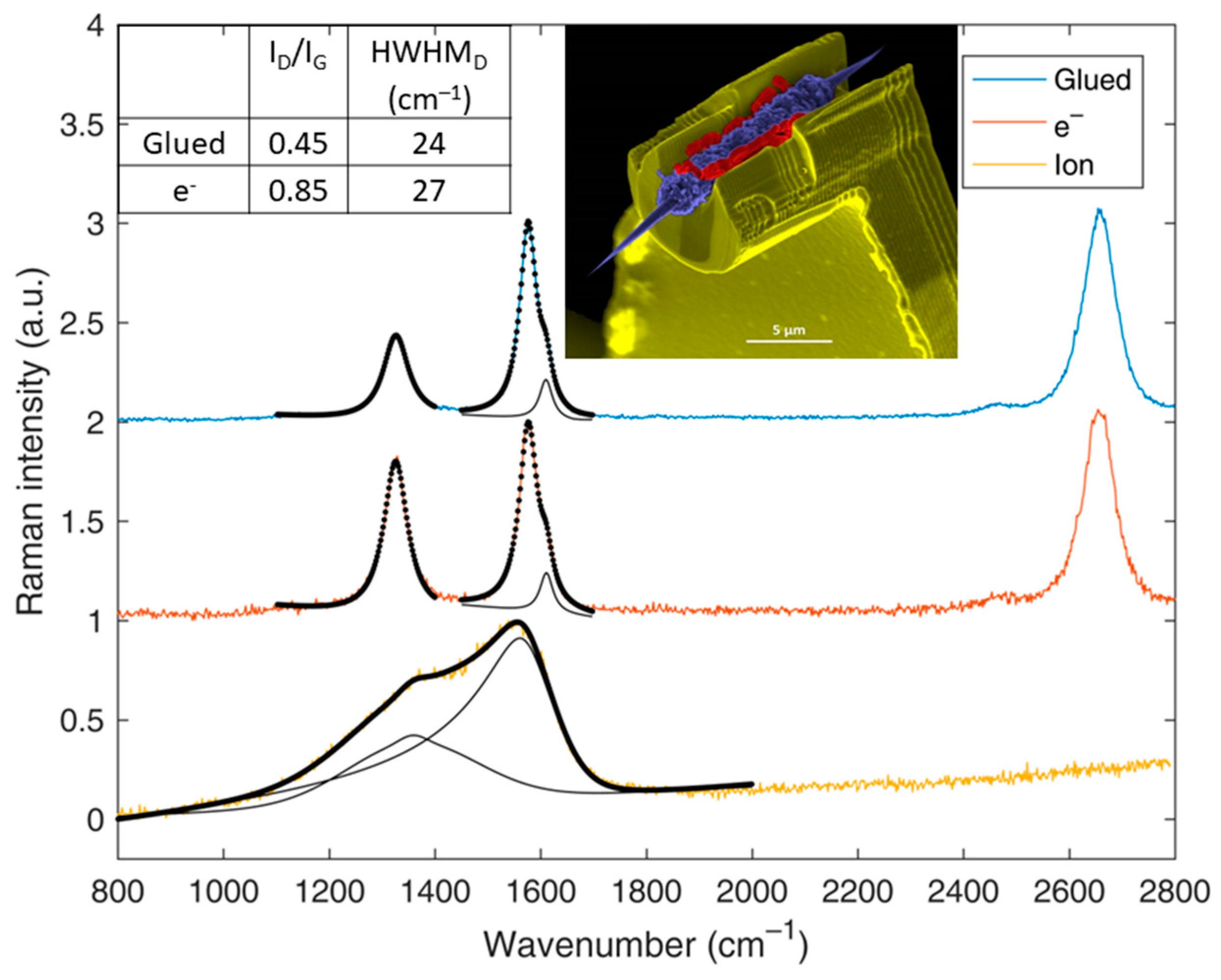
4.2. Single, Quasi-Perfect Graphene: The Case of Isolated Single-Wall Carbon Nanotubes

Up to now, in this paper, going from highly defective to highly organized carbon materials has revealed how the D’ band can be considered. For the D band, the intensity and linewidth are sensitive to disorder but easily adjustable by a double Voigt shape. Unfortunately, this is not always the case and more fundamental analysis may be required to interpret the experimental spectra. We present now the most striking finding obtained in our laboratory on SWCNT by TERS.
In our TERS configuration, we used a silver tip with hot points (see the supplementary information of [34]). Usually, with such a configuration, a metallic substrate has a gap-mode [35]. Here, the carbon nanotube being studied (with diameter around 1.3 nm, hence very likely a single-wall nanotube) was left on its growth substrate, i.e., a flat mica surface (see Section 2.1). The TERS spectrum obtained from it can be seen to be composed of a G band which is split between a G+ (upper wavenumber around 1592 cm−1) and a single G- (lower wavenumber with a position dependent on the diameter) sub-band as shown in Figure 10. The fact that the G- sub-band is single confirms that the nanotube is single-walled. The low wavenumber range is usually used to determine the diameter as the radial breathing mode (RBM) wavenumber is roughly proportional to the inverse of the diameter [36]. When the laser energy meets the optical transition energies (incoming resonance) or the optical transition energies with, in addition, the phonon energy (outcoming resonance), the intensity of the RBM becomes large. Thus, from the couple of these two parameters (RBM wavenumber and photon energy), we can deduce the chirality (n,m) (which characterizes how the graphene sheet rolls up to form the nanotube). [37] With the amount of observations reported over years, accuracy has been improved and effects from the surroundings have been taken into account [38]. In the absence of any distinctive RBM signal (overwhelmed by the signal from the substrate [39]) and knowing the expected range of the nanotube diameter, it is possible to determine accurately the actual nanotube diameter thanks to the value of the wavenumber gap between the G+ and the G- sub-bands. This gap is 49 cm−1, which corresponds to a tube with a diameter of 1.28 nm and a metallic character (if hypothesizing that a semi-conducting tube would correspond to a diameter of 0.99 nm, which is out of the possible range). As the excitation energy is 1.96 eV (633 nm), the Stokes part around the D-G band (1300−1600 cm−1) corresponds to an energy of 1.77−1.80 eV. From the Kataura plot for metallic tubes [40], it corresponds to the (16,1) helicity and the optical transition E 11 M .
What was just made above is a regular way to analyze the Raman spectrum of a SWCNT, for which a TERS is not necessary. However, the TERS spectrum shows much more information for the D band as it exhibits a minimum of five components. The D band overall corresponds to the activation of several phonons, going from 1240 to 1390 cm−1 (hence a spectral range of 150 cm−1). The gap-mode changes the selection of a single D phonon wave-vector. Usually, the D band at this excitation energy is a Lorentzian centered around 1330 cm−1. Here, the wavenumber range is centered to the usual value but its shape is very different. All the phonons in the TO and longitudinal acoustical (LA) branches [41] are not activated as they range from 1175 to 1600 cm−1. From the shift of ordered carbon dωD/dEL = 60 cm−1.eV−1 and from the shape of the Dirac cone E = vFħq where vF is the Fermi velocity, q the electron wave-vector and ħ the reduced Planck constant, we have dωD/dq = 40 cm−1.nm−1. This gives a q range in the reciprocal space of 3.75 nm−1. This value can be compared to the value of the circle in the reciprocal space which is delimited by the Dirac cone and the excitation energy of 2 eV (so 1 eV from the K point) with a radius of E/vFħ = 0.66 nm−1. Due to the double resonance process, the variation of q for a transition from K to K’ is two diameters, which corresponds to 2.6 nm−1. This estimation is satisfactory. We assume that the origin of the peaks is due to the quantification along the circumference. A simple confinement model gives a spacing of 1.54 nm−1 in the reciprocal space for the (16,1) helicity. Consequently, only one line cuts the two circles and this cut is in the middle, giving the two phonons at the edge and other phonons in the intermediate range.
In summary, several peaks can be observed for the D band of a SWCNT due to the quantification around the circumference, and these peaks are well explained by the double resonance theory. Nevertheless, both the linewidth and intensity usually used as parameters to extract the amount of defects are useless in this case. The involved defects are yet to be identified and a possible interaction with the TERS probe should also be considered.

5. Summary

Table 4 summarizes the parameter trends, which were determined by investigating our sample set, and outlines how materials rank over a fairly large range of structural order.
A limit of 2 nm given by Ferrari and Robertson [1] as the La value for which the ID/IG ratio reaches its maximum is indicative of the dependence of the existence of the D band on the content in heteroatoms. Below 2 nm, Ferrari and Robertson propose for the ID/IG ratio a law proportional to La2. In such a picture, the resonance behavior is not considered and is valid for only pure graphenic carbon material. What is important is to attempt to figure out the actual distinction between highly disordered yet graphenic carbons (kerogens, for example, or chars from primary carbonization) and amorphous carbon. In the former case, the contained carbon is certainly combined with a significant amount of other atoms while with amorphous carbon, the sample can be pure carbon and heterogeneous from the point of view of carbon hybridization. Consequently, the Raman spectrum is completely different, for instance with showing a weak D band for amorphous carbon [42]. A large amount of defects can induce the loss of resonant behavior. In such a case, as in kerogens (here exampled by the Barnett and Marcellus49 shales) where the heteroatom content related to the carbon skeleton is fairly high, the D band becomes non-resonant and is no longer due to a double resonance, and, consequently, a local description is probably more appropriate than a crystal description.
A limit of 7 nm is for line defects and concerns a change in the G band linewidth. For large crystallite sizes, if the plane is not perfect with some defect points, a modification of the intensities (see Figure 9) is observed. A TERS analysis also proves that several components should be considered, as in graphite [41].
As a significant content of heteroatoms can heavily influence the Raman response, it might be thought that identifying the specific contribution of each of them (typically O, N, and H) is possible, which would allow the obtaining of some quantification of the atomic composition. However, this is made difficult because of the resonance effect, which can prevail over the non-resonant one.
For oxygen, though, the position of the D band can possibly be correlated [44], but a full study is required to ascertain it.
For nitrogen, parameter trends from Raman spectra have been proposed [45], but applying them to carbon materials with nitrogen content lower than 10% remains an issue.
For hydrogen, some bands corresponding to C−H at 2800 cm−1 to 3300 cm−1 are present, but are close to overtones (D + D’ at 2900 cm−1 and 2D’ at 3200 cm−1). This spectral region is not always studied and moreover is highly sensitive to the excitation energy.
Of course, the above-mentioned possibilities of somehow evaluating the content of O, N, or H require specific materials, such as model ones, to validate the strategies and to be able to extract quantitative data, but in real life, many carbon materials (e.g., kerogens, coke precursors, and chars) exhibit a complex chemical composition to start with and involve all these heteroatoms at once and possibly others. In such a case, solving the problem of the contribution of heteroatoms to the Raman spectra will remain complex for a long time.

6. Conclusions

Raman spectra from kerogens to single-wall carbon nanotubes show a large diversity of D band shapes and more generally highly specific Raman responses, which differ over the whole range of the sample set. As the Raman signal is not proportional to the number of carbon atoms and as the signature is a mixture of different kinds of processes, drawing trends for homogeneous series of samples is possible but expecting a common approach for all kinds of graphenic carbon materials is still challenging.
Parameter trends and laws for different sets of samples have been reported in the literature. To go further, a theory mixing third and fourth perturbation orders in the Raman calculation which correspond to regular and double resonance processes, respectively, is necessary to have a quantitative understanding of the Raman spectrum. It is clear that such a calculation is probably the only way to understand the dependence of Raman spectrum features on so many parameters (e.g., chemical composition, types of defects, crystallite size, crystallite surface functionalization, and so on).

Author Contributions

Investigations: M.K., G.P., N.R.-R., A.K., J.-M.P., P.P., L.M. and E.W.-H.; resources: G.P. and R.P.; methodology: P.P.; writing and discussion: P.P. and M.M.

Funding

A. Kundu acknowledges CEFIPRA for their financial support. M. Kandara and G. Paredes have benefited from the EUR grant NEXT/NanoX (no. ANR-17-EURE-0009) in the framework of the “Programme des Investissements d’Avenir”.

Acknowledgments

V. Jourdain is acknowledged for providing aligned SWCNT on mica (Section 4.2).

Conflicts of Interest

The authors declare no conflict of interest.

References

  1. Ferrari, A.C.; Robertson, J. Interpretation of Raman spectra of disordered and amorphous carbon. Phys. Rev. B 2000, 61, 14095. [Google Scholar] [CrossRef]
  2. Casiraghi, C.; Ferrari, A.C.; Robertson, J. Raman spectroscopy of hydrogenated amorphous carbons. Phys. Rev. B 2005, 72, 085401. [Google Scholar] [CrossRef] [Green Version]
  3. Ferrari, A.C.; Robertson, J. Raman spectroscopy of amorphous, nanostructured, diamond–like carbon, and nanodiamond. Philos. Trans. R. Soc. Lond. Ser. A: Math. Phys. Eng. Sci. 2004, 362, 2477–2512. [Google Scholar] [CrossRef] [PubMed]
  4. Ferrari, A.C.; Robertson, J. Resonant Raman spectroscopy of disordered, amorphous, and diamond-like carbon. Phys. Rev. B 2001, 64, 075414. [Google Scholar] [CrossRef]
  5. Johnson, C.A.; Patrick, J.W.; Thomas, K.M. Characterization of coal chars by Raman spectroscopy, X-ray diffraction and reflectance measurements. Fuel 1986, 65, 1284–1290. [Google Scholar] [CrossRef]
  6. Sadezky, A.; Muckenhuber, H.; Grothe, H.; Niessner, R.; Pöschl, U. Raman microspectroscopy of soot and related carbonaceous materials: Spectral analysis and structural information. Carbon 2005, 43, 1731–1742. [Google Scholar] [CrossRef]
  7. Ferrari, A.C.; Basko, D.M. Raman spectroscopy as a versatile tool for studying the properties of graphene. Nat. Nanotechnol. 2013, 8, 235–246. [Google Scholar] [CrossRef] [Green Version]
  8. Dennison, J.R.; Holtz, M.; Swain, G. Raman spectroscopy of carbon materials. Spectroscopy 1996, 11, 38–45. [Google Scholar]
  9. Lucchese, M.M.; Stavale, F.; Ferreira, E.M.; Vilani, C.; Moutinho, M.V.O.; Capaz, R.B.; Achete, C.A.; Jorio, A. Quantifying ion-induced defects and Raman relaxation length in graphene. Carbon 2010, 48, 1592–1597. [Google Scholar] [CrossRef]
  10. Cançado, L.G.; Da Silva, M.G.; Ferreira, E.H.M.; Hof, F.; Kampioti, K.; Huang, K.; Pénicaud, A.; Achete, C.A.; Capaz, R.B.; Jorio, A. Disentangling contributions of point and line defects in the Raman spectra of graphene-related materials. 2D Mater. 2017, 4, 025039. [Google Scholar] [CrossRef]
  11. Tuinstra, F.; Koenig, J.L. Raman spectrum of graphite. J. Chem. Phys. 1970, 53, 1126–1130. [Google Scholar] [CrossRef]
  12. Cançado, L.G.; Jorio, A.; Pimenta, M.A. Measuring the absolute Raman cross section of nanographites as a function of laser energy and crystallite size. Phys. Rev. B 2007, 76, 064304. [Google Scholar] [CrossRef]
  13. Mallet-Ladeira, P.; Puech, P.; Toulouse, C.; Cazayous, M.; Ratel-Ramond, N.; Weisbecker, P.; Vignoles, G.L.; Monthioux, M. A Raman study to obtain crystallite size of carbon materials: A better alternative to the Tuinstra–Koenig law. Carbon 2014, 80, 629–639. [Google Scholar] [CrossRef]
  14. Thomsen, C.; Reich, S. Double resonant Raman scattering in graphite. Phys. Rev. Lett. 2000, 85, 5214–5217. [Google Scholar] [CrossRef] [PubMed]
  15. Allouche, H.; Monthioux, M.; Jacobsen, R.L. Chemical vapor deposition of pyrolytic carbon on carbon nanotubes: Part 1. Synthesis and morphology. Carbon 2003, 41, 2897–2912. [Google Scholar] [CrossRef]
  16. Asadullah, M.; Zhang, S.; Min, Z.; Yimsiri, P.; Li, C.Z. Effects of biomass char structure on its gasification reactivity. Bioresour. Technol. 2010, 101, 7935–7943. [Google Scholar] [CrossRef] [PubMed]
  17. Mallet-Ladeira, P.; Puech, P.; Weisbecker, P.; Vignoles, G.L.; Monthioux, M. Behavior of Raman D band for pyrocarbons with crystallite size in the 2–5 nm range. Appl. Phys. A 2014, 114, 759–763. [Google Scholar] [CrossRef]
  18. Fung, A.W.P.; Rao, A.M.; Kuriyama, K.; Dresselhaus, M.S.; Dresselhaus, G.; Endo, M.; Shindo, N. Raman scattering and electrical conductivity in highly disordered activated carbon fibers. J. Mater. Res. 1993, 8, 489–500. [Google Scholar] [CrossRef] [Green Version]
  19. Merlen, A.; Buijnsters, J.; Pardanaud, C. A guide to and review of the use of multiwavelength Raman spectroscopy for characterizing defective aromatic carbon solids: From graphene to amorphous carbons. Coatings 2017, 7, 153. [Google Scholar] [CrossRef]
  20. Puech, P.; Dabrowska, A.; Ratel-Ramond, N.; Vignoles, G.L.; Monthioux, M. New insight on carbonisation and graphitisation mechanisms as obtained from a bottom-up analytical approach of X-ray diffraction patterns. Carbon 2019, 147, 602–611. [Google Scholar] [CrossRef]
  21. Cançado, L.G.; Jorio, A.; Ferreira, E.M.; Stavale, F.; Achete, C.A.; Capaz, R.B.; Moutinho, M.V.O.; Lombardo, A.; Kulmala, T.S.; Ferrari, A.C. Quantifying defects in graphene via Raman spectroscopy at different excitation energies. Nano Lett. 2011, 11, 3190–3196. [Google Scholar] [CrossRef] [PubMed]
  22. Cançado, L.G.; Takai, K.; Enoki, T.; Endo, M.; Kim, Y.A.; Mizusaki, H.; Jorio, A.; Coelho, L.N.; Magalhães-Paniago, R.; Pimenta, M.A. General equation for the determination of the crystallite size La of nanographite by Raman spectroscopy. Appl. Phys. Lett. 2006, 88, 163106. [Google Scholar] [CrossRef]
  23. Beyssac, O.; Goffé, B.; Chopin, C.; Rouzaud, J.N. Raman spectra of carbonaceous material in metasediments: A new geothermometer. J. Metamorph. Geol. 2002, 20, 859–871. [Google Scholar] [CrossRef]
  24. Guizani, C.; Jeguirim, M.; Gadiou, R.; Sanz, F.J.E.; Salvador, S. Biomass char gasification by H2O, CO2 and their mixture: Evolution of chemical, textural and structural properties of the chars. Energy 2016, 112, 133–145. [Google Scholar] [CrossRef]
  25. Schmid, J.; Grob, B.; Niessner, R.; Ivleva, N.P. Multiwavelength Raman microspectroscopy for rapid prediction of soot oxidation reactivity. Anal. Chem. 2011, 83, 1173–1179. [Google Scholar] [CrossRef]
  26. Puech, P.; Plewa, J.M.; Mallet-Ladeira, P.; Monthioux, M. Spatial confinement model applied to phonons in disordered graphene-based carbons. Carbon 2016, 105, 275–281. [Google Scholar] [CrossRef]
  27. Romero-Sarmiento, M.F.; Rouzaud, J.N.; Bernard, S.; Deldicque, D.; Thomas, M.; Littke, R. Evolution of Barnett Shale organic carbon structure and nanostructure with increasing maturation. Org. Geochem. 2014, 71, 7–16. [Google Scholar] [CrossRef]
  28. Dopita, M.; Rudolph, M.; Salomon, A.; Emmel, M.; Aneziris, C.G.; Rafaja, D. Simulations of X-Ray Scattering on TwoDimensional, Graphitic and Turbostratic Carbon Structures. Adv. Eng. Mater. 2013, 15, 1280–1291. [Google Scholar] [CrossRef]
  29. Robertson, J. Photoluminescence mechanism in amorphous hydrogenated carbon. Diam. Relat. Mater. 1996, 5, 457–460. [Google Scholar] [CrossRef]
  30. Pillet, G.; Sapelkin, A.; Bacsa, W.; Monthioux, M.; Puech, P. Size-controlled graphene-based materials prepared by annealing of pitch-based cokes: G band phonon line broadening effects due to high pressure, crystallite size, and merging with D′ band. J. Raman Spectrosc. 2019, in press. [Google Scholar] [CrossRef]
  31. Eckmann, A.; Felten, A.; Mishchenko, A.; Britnell, L.; Krupke, R.; Novoselov, K.S.; Casiraghi, C. Probing the nature of defects in graphene by Raman spectroscopy. Nano Lett. 2012, 12, 3925–3930. [Google Scholar] [CrossRef] [PubMed]
  32. Audier, M.; Oberlin, A.; Oberlin, M.; Coulon, M.; Bonnetain, L. Morphology and crystalline order in catalytic carbons. Carbon 1981, 19, 217–224. [Google Scholar] [CrossRef]
  33. Allouche, H.; Monthioux, M. Chemical vapor deposition of pyrolytic carbon on carbon nanotubes. Part. II: Texture and structure. Carbon 2005, 43, 1265–1278. [Google Scholar] [CrossRef]
  34. Su, W.; Kumar, N.; Krayev, A.; Chaigneau, M. In situ topographical chemical and electrical imaging of carboxyl graphene oxide at the nanoscale. Nat. Commun. 2018, 9, 2891. [Google Scholar] [CrossRef]
  35. Richard-Lacroix, M.; Zhang, Y.; Dong, Z.; Deckert, V. Mastering high resolution tip-enhanced Raman spectroscopy: Towards a shift of perception. Chem. Soc. Rev. 2017, 46, 3922–3944. [Google Scholar] [CrossRef]
  36. Rao, A.M.; Richter, E.; Bandow, S.; Chase, B.; Eklund, P.C.; Williams, K.A.; Fang, S.; Subbaswamy, K.R.; Menon, M.; Thess, A.; et al. Diameter-selective Raman scattering from vibrational modes in carbon nanotubes. Science 1997, 275, 187–191. [Google Scholar] [CrossRef]
  37. Jorio, A.; Saito, R.; Hafner, J.H.; Lieber, C.M.; Hunter, D.M.; McClure, T.; Dresselhaus, G.; Dresselhaus, M.S. Structural (n, m) determination of isolated single-wall carbon nanotubes by resonant Raman scattering. Phys. Rev. Lett. 2001, 86, 1118. [Google Scholar] [CrossRef]
  38. Araujo, P.T.; Pesce, P.B.C.; Dresselhaus, M.S.; Sato, K.; Saito, R.; Jorio, A. Resonance Raman spectroscopy of the radial breathing modes in carbon nanotubes. Phys. E Low-Dim. Syst. Nanostruct. 2010, 42, 1251–1261. [Google Scholar] [CrossRef]
  39. Jorio, A.; Souza Filho, A.G.; Dresselhaus, G.; Dresselhaus, M.S.; Swan, A.K.; Ünlü, M.S.; Goldberg, B.B.; Pimenta, M.A.; Hafner, J.H.; Lieber, C.M.; et al. G-band resonant Raman study of 62 isolated single-wall carbon nanotubes. Phys. Rev. B 2002, 65, 155412. [Google Scholar] [CrossRef]
  40. Telg, H.; Maultzsch, J.; Reich, S.; Hennrich, F.; Thomsen, C. Chirality distribution and transition energies of carbon nanotubes. Phys. Rev. Lett. 2004, 93, 177401. [Google Scholar] [CrossRef]
  41. Maultzsch, J.; Reich, S.; Thomsen, C. Double-resonant Raman scattering in graphite: Interference effects, selection rules, and phonon dispersion. Phys. Rev. B 2004, 70, 155403. [Google Scholar] [CrossRef] [Green Version]
  42. Chhowalla, M.; Ferrari, A.C.; Robertson, J.; Amaratunga, G.A.J. Evolution of sp2 bonding with deposition temperature in tetrahedral amorphous carbon studied by Raman spectroscopy. Appl. Phys. Lett. 2000, 76, 1419–1421. [Google Scholar] [CrossRef]
  43. Zhang, L.; Wei, X.; Lin, Y.; Wang, F. A ternary phase diagram for amorphous carbon. Carbon 2015, 94, 202–213. [Google Scholar] [CrossRef]
  44. Pillet, G.; Freire-Soler, V.; Eroles, M.N.; Bacsa, W.; Dujardin, E.; Puech, P. Reversibility of defect formation during oxygen-assisted electron-beam-induced etching of graphene. J. Raman Spectrosc. 2018, 49, 317–323. [Google Scholar] [CrossRef]
  45. Ferrari, A.C.; Rodil, S.E.; Robertson, J. Interpretation of infrared and Raman spectra of amorphous carbon nitrides. Phys. Rev. B 2003, 67, 155306. [Google Scholar] [CrossRef] [Green Version]
Figure 1. Typical Raman spectrum (black line) for a disordered carbon showing the principle of hand-made measurement of the half width at half maximum (HWHM). HWHMD (HWHMD) is for the D band (G band respectively). The G and D band contributions are plotted in red. The dotted blue reports the D band decomposition in two Voigt sub-bands (same wavenumber).
Carbon 05 00069 g001
Figure 2. Raman spectra of the Barnett gas-shale obtained with an excitation wavelength of (a) 336 nm and (b) 532 nm. The fitting and its components (black lines) are also shown but the sub-bands are not represented for clarity. (c) and (d) show comparisons of both previous spectra (blue: 336 nm spectrum; green: 532 nm spectrum) while normalizing them using the G band intensity (c) and the D band intensity (d). The vertical lines represent the position of the D band for graphite for each excitation energy.
Carbon 05 00069 g002
Figure 3. Raman spectra of the Marcellus49 gas-shale obtained with an excitation wavelength of (a) 336 nm and (b) 532 nm. The fitting (red line) and its components (blue lines) are also shown. (c) and (d) show comparisons of both spectra (blue: 336 nm spectrum; green: 532 nm spectrum) while normalizing them using the G band intensity (c) and the D band intensity (d). The vertical lines represent the position of the D band for graphite for each excitation energy.
Carbon 05 00069 g003
Figure 4. X-ray diffractogram (left: 002 region; right: 10 region) of the N330 carbon black before and after being incorporated into a model tire and then subjected to two recycling processes. The sharper and intense peaks seen on the right shoulder of both the 002 and the 10 peaks are due to leftovers of other phases involved in the tire fabrication. La is the in-plane diameter of the crystallite size while Lc is its height.
Carbon 05 00069 g004
Figure 5. Raman spectra with their fitting (red lines are the components of the fit; blue lines are the resulting fit) for the three N330 samples (from top to bottom, the ranking is the same as in Figure 4). Left: green excitation; right: red excitation.
Carbon 05 00069 g005
Figure 6. Raman spectra of annealed cokes (left: 1300 °C; right: 1900 °C) for two excitation wavelengths. The fits are the solid black line.
Carbon 05 00069 g006
Figure 7. High resolution transmission electron microscopy (HRTEM) image of the nano-sized apex of an all-graphene carbon cone. Dots are carbon atoms. Several examples of buckling graphenes forming loops are seen. (Photo credit: R. Wang, CEMES-CNRS).
Carbon 05 00069 g007
Figure 8. Raman spectra (the D’ contribution to the fit is also plotted as the thin, solid black line) of a carbon cone at the various positions indicated on the image in the inset. Top left: values of both ID/IG and ID/ID’ ratios.
Carbon 05 00069 g008
Figure 9. Raman spectra (with fitting as the heavy, black solid line) recorded on the microfiber part of three different carbon cones mounted onto an AFM cantilever (an example is provided in the inset: purple-blue is the (cone+ short microfiber segment) carbon morphology; yellow is the Si-doped cantilever support; and red is the welding material, here an ion-promoted Pt deposit) by the three different procedures described in the text: bottom (blue line) Pt deposition promoted by focused ions; middle (red line) Pt deposition promoted by focused electrons; and top (yellow line) gluing with a UV-curable resin. In the top-left inset are provided the ID/IG height ratio as well as the linewidth of the D band for the two cones still exhibiting the regular D + G (+ 2D) bands. Indeed, the apex of the cone subjected to an ion beam during the mounting (blue line) has been heavily transformed and is no longer graphenic but amorphous, yet it does not show up as low magnification (see the cone apex in the middle-top image showing a cone welded onto the Si-doped cantilever support).
Carbon 05 00069 g009
Figure 10. Tip-enhanced Raman scattering spectrum of a single-wall carbon nanotube with the silver tip in close vicinity to the surface. The fitting for the G and G+ is indicated with dots.
Carbon 05 00069 g010
Table 1. Fitting parameters corresponding to Figure 1 and Figure 2.
Sampleλ
(nm)
ωD
(cm−1)
ωG
(cm−1)
HWHMD
(cm−1)
HWHMG
(cm–1)
ID/IGD/dEL
(cm−1.eV–1)
α
See Equation (1)
Barnett
Gas and oil
3361388161043240.37181.1
5321364159252260.61
Marcellus49
Gas
3361374160839170.44260.6
5321339160146120.59
Table 2. Fitting parameters corresponding to Figure 5. Wavelengths of 532 and 633 nm correspond to energy of 2.33 and 1.96 eV, respectively.
Sampleλ (nm)ωD
(cm−1)
ωG
(cm−1)
HWHMD
(cm−1)
HWHMG
(cm−1)
ID/IGD/dEL
(cm−1.eV−1)
α
Steam53213131601144421.051273.7
63313601594125461.98
Pyro53213571603127450.99491.3
63313391597133561.24
N33053213441589119531.23270.14
63313341601109501.26
Table 3. ID/ID’ ratio value as a function of the type of defects. * values correspond to the work by Eckmann et al. [31].
Type of DefectsID/ID’
sp313*
Vacancy7*
Boundary3.5*
Loop1.5 (our result)
Table 4. Trends of evolution with crystallite size of the three main parameters associated with a Raman spectrum.
La<2 nm2–7 nm>7 nm
ID/IGFor amorphous carbon (a-C): proportional to La2 [1]Varies roughly with 1/La (see Equation (2)) and is affected by the presence of heretoatoms (see Section 3)ID/ID’ to be considered (see Section 4).
Experimental laws for ID/IG (see Equations (2) and (3) for the least)
For disordered-C: varies with the content in chain, defects, and heteroatoms [3]
HWHMDOne component.
Is dependent on both dωD/dE and 1/La.
Could reach a maximum (see Section 3)
Often two different components [17]. Varies with 1/La [26]Varies roughly with 1/La [26]
HWHMGFor a-C: decreases with increased La [42]Varies with 1/La or La (because the La size range is small) [13]Jumps due to the merging of G and D’ around 7 nm [30]. Weak dependence for larger La
For disordered-C: varies with the content in chain, defects, and heteroatoms [43]

