A Study on the Effect of Carbon Nanotubes’ Distribution and Agglomeration in the Free Vibration of Nanocomposite Plates


1
CIMOSM, ISEL, Centro de Investigação em Modelação e Optimização de Sistemas Multifuncionais, 1959-007 Lisbon, Portugal
2
IDMEC, IST—Instituto Superior Técnico, Universidade de Lisboa, 1049-001 Lisbon, Portugal
3
UNIDEMI, Departamento de Engenharia Mecânica e Industrial, Faculdade de Ciências e Tecnologia, Universidade NOVA de Lisboa, 2829-516 Caparica, Portugal
*
Authors to whom correspondence should be addressed.
C 2020, 6(4), 79; https://0-doi-org.brum.beds.ac.uk/10.3390/c6040079
Submission received: 3 November 2020
/
Revised: 18 November 2020
/
Accepted: 23 November 2020
/
Published: 30 November 2020
(This article belongs to the Collection Feature Papers in the Science and Engineering of Carbons)
Abstract
:The present work aimed to characterize the free vibrations’ behaviour of nanocomposite plates obtained by incorporating graded distributions of carbon nanotubes (CNTs) in a polymeric matrix, considering the carbon nanotubes’ agglomeration effect. This effect is known to degrade material properties, therefore being important to predict the consequences it may bring to structures’ mechanical performance. To this purpose, the elastic properties’ estimation is performed according to the two-parameter agglomeration model based on the Eshelby–Mori–Tanaka approach for randomly dispersed nano-inclusions. This approach is implemented in association with the finite element method to determine the natural frequencies and corresponding mode shapes. Three main agglomeration cases were considered, namely, agglomeration absence, complete agglomeration, and partial agglomeration. The results show that the agglomeration effect has a negative impact on the natural frequencies of the plates, regardless the CNTs’ distribution considered. For the corresponding vibrations’ mode shapes, the agglomeration effect was shown in most cases not to have a significant impact, except for two of the cases studied: for a square plate and a rectangular plate with symmetrical and unsymmetrical CNTs’ distribution, respectively. Globally, the results confirm that not accounting for the nanotubes’ agglomeration effect may lead to less accurate elastic properties and less structures’ performance predictions.
1. Introduction
Carbon nanotubes’ (CNTs) remarkable characteristics makes them well suited for acting as a reinforcing phase in composite materials where high strength and low density are required or in applications where superior physical, mechanical, thermal, and electrical properties have to be guaranteed [1,2]. Considering these nanoparticles’ potential use in a number of engineering fields, it is thus important to characterize the influence that their distribution and eventual agglomeration may have in the behaviour of structures, namely in their free vibrations’ behaviour.
A number of researchers have developed very relevant work in the field of composite materials reinforced with nanoparticles. Among them, one can refer the work developed by Sobhani Aragh et al. [3], where an equivalent continuum model based on the Eshelby–Mori–Tanaka (EMT) approach was employed to estimate the elastic properties of functionally graded carbon nanotube-reinforced composite (FG-CNTRC) cylindrical panels to study their free vibration response. These authors found out that CNTs’ volume fraction can be used for the management of vibrational behaviour of structures. A similar study was developed by Sobhadi Aragh et al. [4], this time using the third-order shear deformation theory to investigate the dynamic behaviour of FG-CNTRCs cylindrical shells. These authors concluded that symmetric distributions of the CNTs’ volume fraction, over the thickness direction, provided a greater improvement of the dynamic behaviour when compared to uniform or unsymmetrical volume fraction distributions. Yas and Heshmati [5] studied the influence of various CNTs distributions and orientations, among other parameters on the dynamic behaviour of a functionally graded nanocomposite Timoshenko beam.
Due to their high aspect ratio, low bending stiffness, and van der Waals forces, CNTs tend to agglomerate into bundles [6,7], with this phenomenon interfering directly with the material properties of a CNTRC (carbon nanotube-reinforced composite). To estimate the CNTRC’s properties more realistically, it is necessary to take into account this agglomeration effect. However, in most of the studies including CNTRC, the most common homogenization scheme employed is the extended rule of mixtures (ROM) not taking into account this effect.
To overcome this problem, Shi et al. [8] proposed a two-parameter agglomeration model based on the EMT for CNTRC property estimation with randomly oriented straight CNTs to investigate the effect of nanotube waviness and agglomeration on the mechanical properties of CNTRCs.
Van der Waals forces play an important role on CNT micromechanical models namely, to model the interphase between the resin and the CNT for nanocomposites, for predicting their mechanical properties as proposed in the studies led by Shokrieh [9,10]. There is another important consideration about the van der Waals forces when assessing the free vibration behaviour of MWCNT (multi-walled carbon nanotubes), which is the interaction of the van der Waals forces between two different SWCNT (single-walled carbon nanotube) layers and their effect on the natural frequencies and modes’ shapes. The study developed by He et al. [11] indicated that when considering van der Waals forces, the modes’ shapes change when varying the radii in MWCNT from very small to very large, and the that these forces have a significant impact in higher natural frequencies. Another study that considers the influence of the van der Waals forces between two different SWCNT layers is the study developed by Strozzi and Pellicano [12] on the linear vibrations of TWCNTs (triple-walled carbon nanotubes), where these interactions are modelled by means of a radius-dependent function that relates the displacements of two adjacent layers.
Since the EMT agglomeration model was proposed, a number of studies have emerged using this technique for property estimation. Among them, the dynamic behaviour of an FG-CNTRC Timoshenko beam resting on a Pasternak foundation was studied under the influence of CNT agglomeration, showing that the natural frequencies of the beam are highly influenced by the agglomeration effect [13]. Another study performed using beam models was developed by Heshmati and Yas [14], where the dynamic behaviour of FG nanocomposite beams was evaluated under the influence of CNT agglomeration, and it was also shown that the agglomeration exerted a significant weakening effect in CNTRC.
Kamarian et al. [15] studied the dynamic behaviour under free vibrations of CNTRC conical shells under the influence of agglomerated CNT using the EMT approach and they concluded that the agglomeration significantly affects the natural frequency of the structure. Tornabene et al. [16] performed a study on the effect of agglomerated CNTs on the natural frequencies of FG-CNTRC doubly curved shells, where several parametric studies were developed varying the CNT volume fraction, the CNTs distributions along the thickness, as well as the agglomeration parameters, proving their influence on the dynamic behaviour of the structure. Tornabene et al. [17] published another study now on the static response of nanocomposite plates and shells reinforced by agglomerated CNTs, where the static response of these structures was shown to be considerably affected by the agglomeration of CNTs.
Eringen’s nonlocal elasticity theory was employed to develop bending and buckling analyses of agglomerated CNTRC nanoplates resting on a Pasternak foundation by Daghigh et al. [18]. With this study, it was concluded that the presence of the foundation beneath the nanoplates reduced the effects of CNT agglomeration. The same author led another study on the dynamic behaviour of size- and temperature-dependent agglomerated CNTRC nanoplates resting on a visco-Pasternak foundation [19], where it was concluded that ignoring the agglomeration effect causes an overestimation of the elastic properties and the presence of the Pasternak foundation clearly increased the nanoplate natural frequency.
More recently, Bisheh et al. [20] studied the dynamics of wave propagation in agglomerated CNTR piezoelectric composite cylindrical shells. The developed analytical model showed a capacity to find the effects of nanotube agglomeration on wave propagation characteristics of these smart nanocomposite shells for the applications of structural health monitoring and energy harvesting. The performance of CNTR porous composite plates bonded with piezoceramic material in the lower and upper faces under static mechanical and electrical loading was evaluated by Moradi-Dastjerdi et al. [21], concluding that embedding pores up to around 90% of the volume of the middle plate leads to an increase of around 11.3% and 2.2% in mechanical and electrical deflections, respectively. The inclusion of CNTs in the middle plate was demonstrated to be beneficial; however, this was to limited values of the CNT volume fraction due to the agglomeration effect.
A modelling paradigm for improving the piezoelectric performance for piezoelectric matrix-inclusion composites based on lead-free ceramics through improved matrices and optimal polycrystallinity in the piezoelectric inclusions was developed by Krishnaswamy et al. [22]. These authors demonstrated for this case that CNT agglomeration near nanotube percolation and the clustering of nanotubes can lead to better matrix hardening and higher permittivity, leading to an improvement exceeding 30% in piezoelectric response.
As mentioned, CNTs have remarkable characteristics that are important for many engineering applications; however, CNTs tend to agglomerate even for low volume fraction’s distributions [23]. Hence, assessing the influence of the agglomeration effect on the free vibration behaviour of nanocomposites is fundamental to better design structures built from these materials. The present work aimed to characterize the free vibration behaviour of FG-CNTRC square and rectangular plates concerning the effect of CNTs’ distributions and agglomeration, regarding its influence on the natural frequencies and modes’ shapes of these plate-type structures.
2. Materials and Methods
The present section is subdivided into two sub-sections, wherein the most relevant aspects, techniques, and methodologies that support the present study are summarized.
2.1. Properties’ Estimation through the Eshelby–Mori–Tanaka Approach
In FG-CNTs, CNTs tend to agglomerate in a polymer matrix, due to its high aspect ratio, low bending stiffness (small diameter and lower elastic modulus in its radial direction), and to van der Waals forces. Shi et al. [8] developed a two-parameter model to describe the effect of agglomeration on the elastic properties of randomly oriented CNTs.
The present Eshelby–Mori–Tanaka property estimation model [8] is based on the equivalent fibre concept. The equivalent fibre properties are estimated by multiscale finite element method (FEM) analysis or through molecular dynamics (MD) simulations. Through these simulations, one determines the properties of the composite, and then the properties of the equivalent fibre might be calculated using the rule of mixtures (ROM) presented in Equation (1). A virtual-equivalent fibre consists of a straight CNT embedded in a polymeric resin and its interphase. For the SWCNT with a chiral index of (10,10), the equivalent fibre would be a solid cylinder with a 1.424-nm diameter [10]. The properties of the equivalent fibre for the present studies are listed in Table 1.
where , , , and are the longitudinal elastic modulus, transverse elastic modulus, shear modulus, and Poisson’s ratio, respectively, of the equivalent fiber. , , , and are the longitudinal elastic modulus, transverse elastic modulus, shear modulus, and Poisson’s ratio, respectively, of the composite, which were determined using multiscale FEM or MD simulations. , , and are the elastic modulus, shear modulus, and Poisson’s ratio, respectively, of the matrix. Finally, and are the volume fraction of the equivalent fibre and the volume fraction of the matrix, respectively.
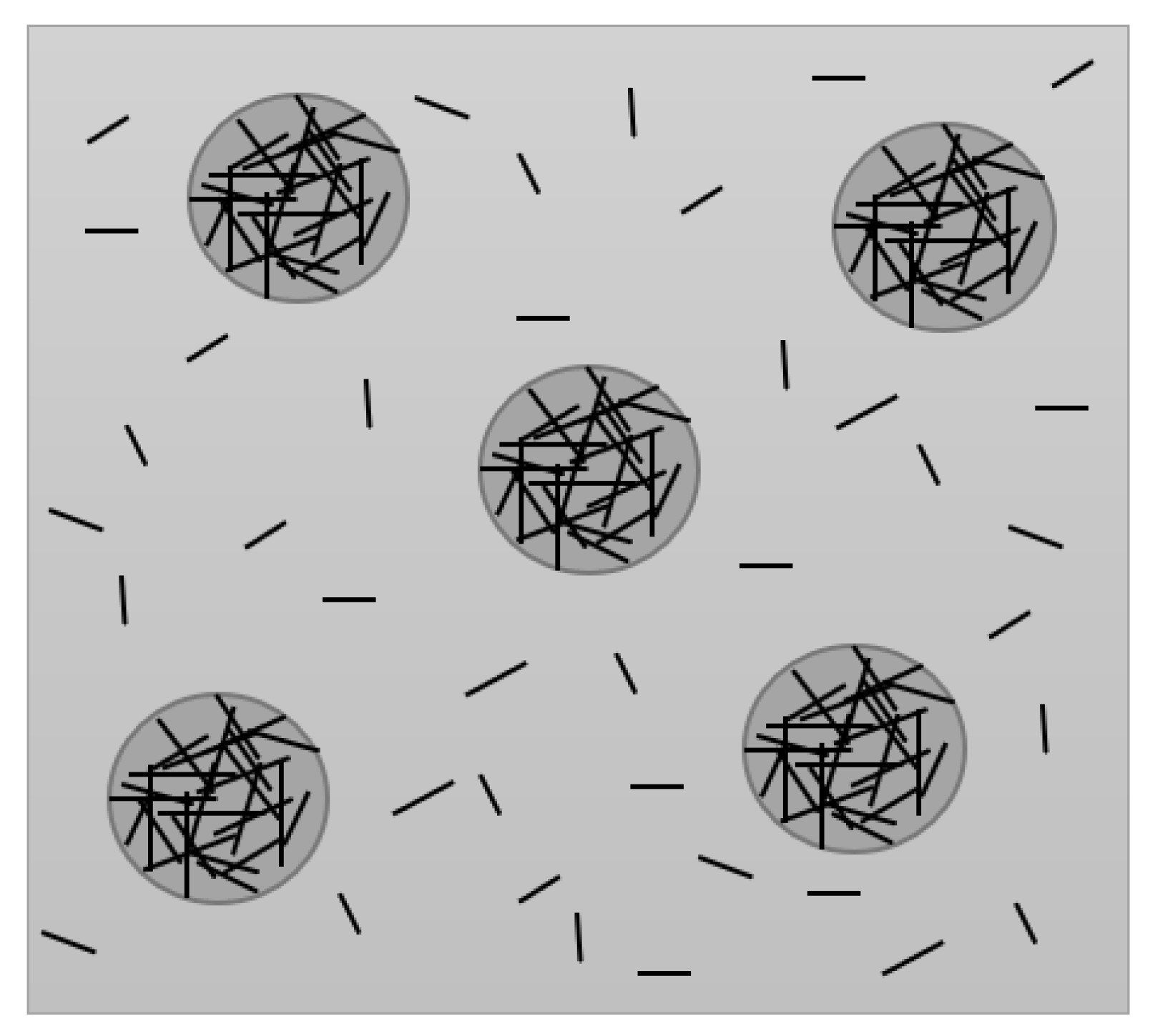
This model considers that a part of the CNTs’ reinforcement is dispersed throughout the matrix, while another part appears in a cluster form due to the agglomeration effect. This model is based on the Eshelby inclusion model, where it is assumed that the inclusions appear in spherical shapes and they are represented in Figure 1 [13]. The total volume of CNT reinforcement in the representative volume element (RVE) is denoted by and is divided in , which is the volume of CNTs in the agglomerated inclusions, and , which is the volume of CNTs dispersed in the matrix. Note that from now on, the subscripts and will stand for the reinforcing phase and for the matrix, respectively. The employed homogenization scheme here described can be originally found in Section 4.1 of the reference article [8].
The two parameters used to describe the agglomeration are and , where denotes the volume fraction of the inclusions with respect to the volume of the RVE, is the volume ratio of CNTs that are dispersed in agglomerated inclusions with respect to the total volume of CNTs , and where is the total volume of the inclusions within the RVE:
when , all the CNTs are uniformly dispersed in the matrix. With the decrease of , the agglomeration degree is more severe. If , all the CNTs are located within the agglomerated inclusions. If , then the volume fraction of CNTs inside the inclusions is the same as the volume fraction CNTs outside, which means the CNTs are uniformly distributed. When and the bigger the value of , the spatial distribution of CNTs throughout the matrix is more heterogeneous.
The average volume fraction of CNTs in the composite is described by:
Although assuming the nanotubes are transversely isotropic, considering that the nanotubes are randomly dispersed within the inclusions as well as within the matrix, one might consider that the material behaves as an isotropic material inside and outside the inclusions.
Using the Mori–Tanaka method for composite properties’ estimation for randomly oriented CNTs and considering the agglomeration effect, one has:
where , , , , and are Hill’s elastic moduli calculated by the inverse of the compliance matrix of the equivalent fibre. Note that , , , , , , and are its properties, which can be determined using ROM, but first the properties of the composite must be determined using a multiscale FEM or an MD simulation analysis [13].
The Hill’s elastic moduli are used to determine the effective bulk moduli of the composite inside the inclusions and outside the inclusions , and the same goes for the shear moduli inside and outside the inclusions ( and , respectively) [8]:
where:
The bulk and shear moduli of the matrix are and , respectively. Finally, the effective bulk modulus and the effective shear modulus of the composite can be determined using the following expressions:
where:
where is the Poisson’s ratio outside the inclusions. Finally, one can determine the effective Young modulus and Poisson’s ratio of the composite using:
Besides using the EMT agglomeration model to estimate the elastic properties of the FG-CNTRC, the composite mass density is calculated using the Voigt’s rule [24,25]:
where and are the matrix volume fraction and mass density, respectively. The matrix volume fraction is given by .
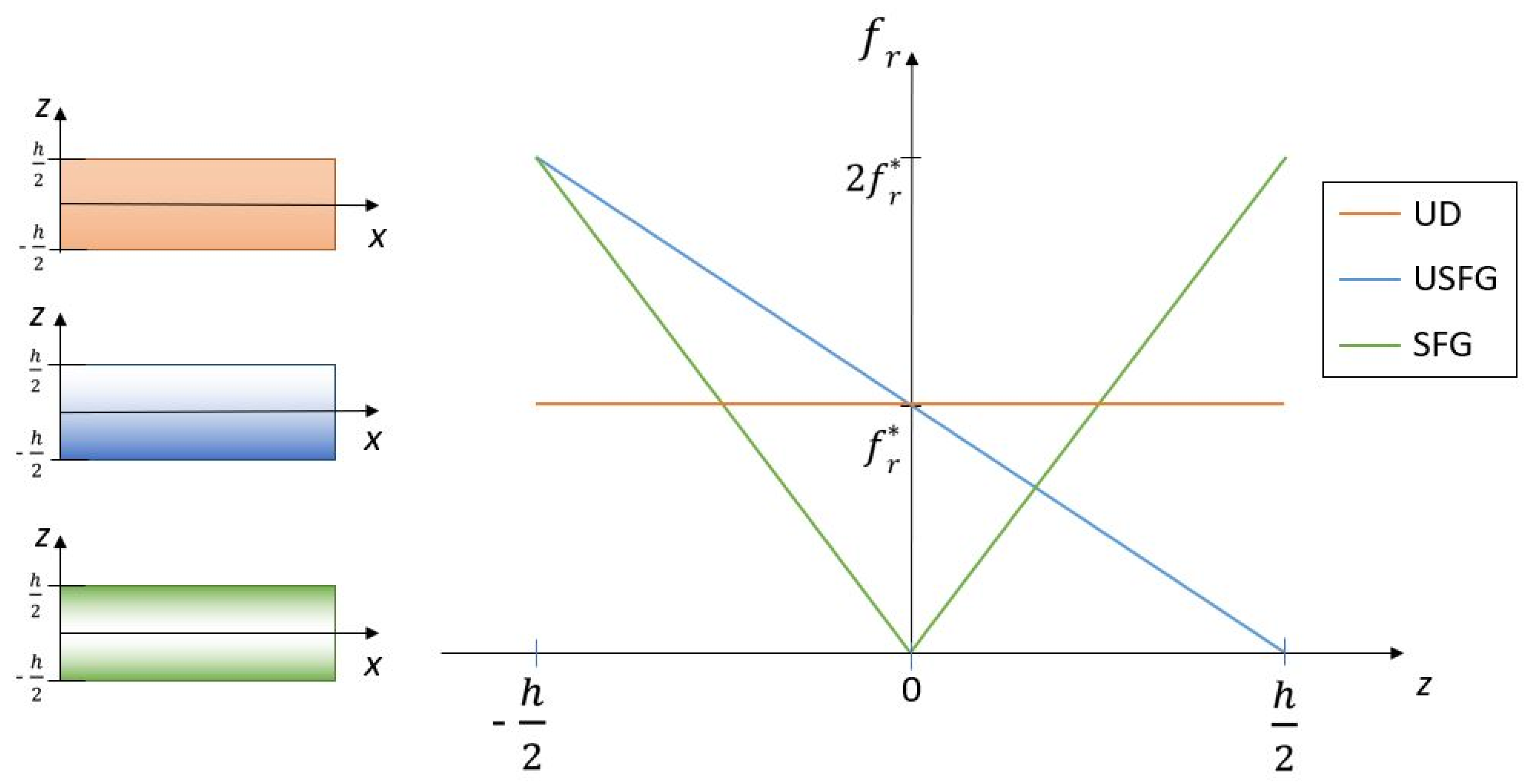
To calculate the mentioned properties, one must define how the CNTs are distributed along the matrix in the FG-CNTRC. For this purpose, three different CNTs volume fractions distributions were considered in this work, these volume fraction distributions are represented in Figure 2. The first is the uniform distribution (UD):
An unsymmetrical functionally graded distribution (USFG) of the CNTs:
A symmetrical functionally graded distribution (SFG) of the CNTs:
Knowing that , where is the FG-CNTRC thickness and in which is defined by [5]:
where is the mass fraction of the carbon nanotubes.
2.2. Free Vibration Analysis
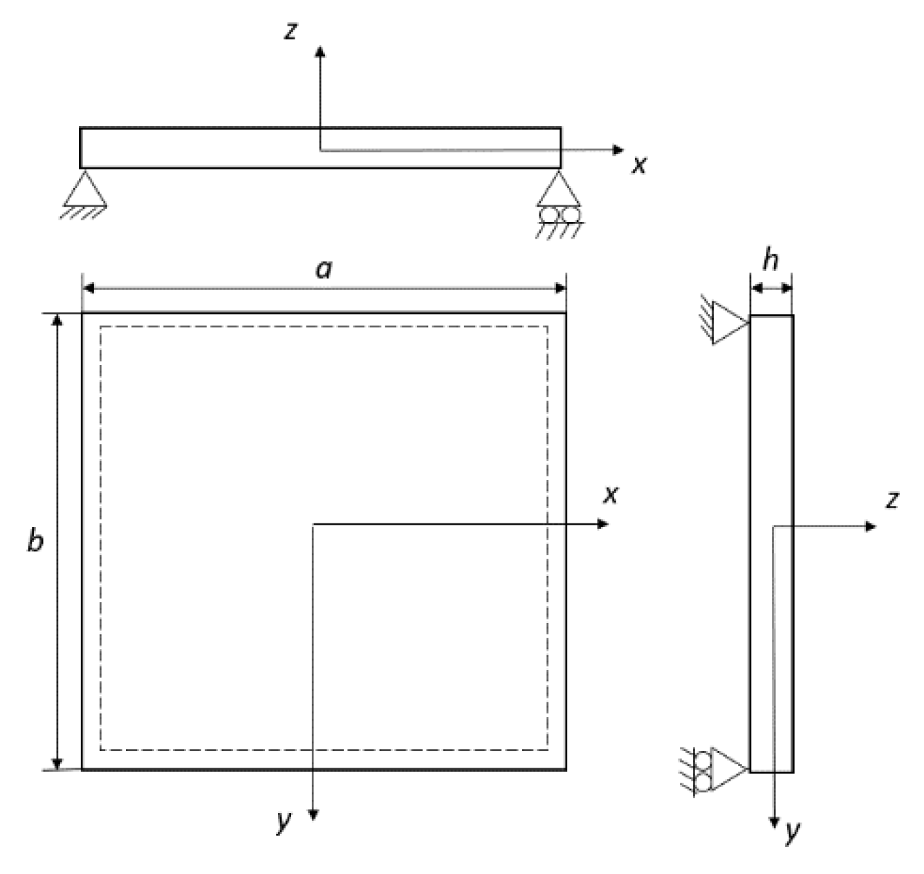
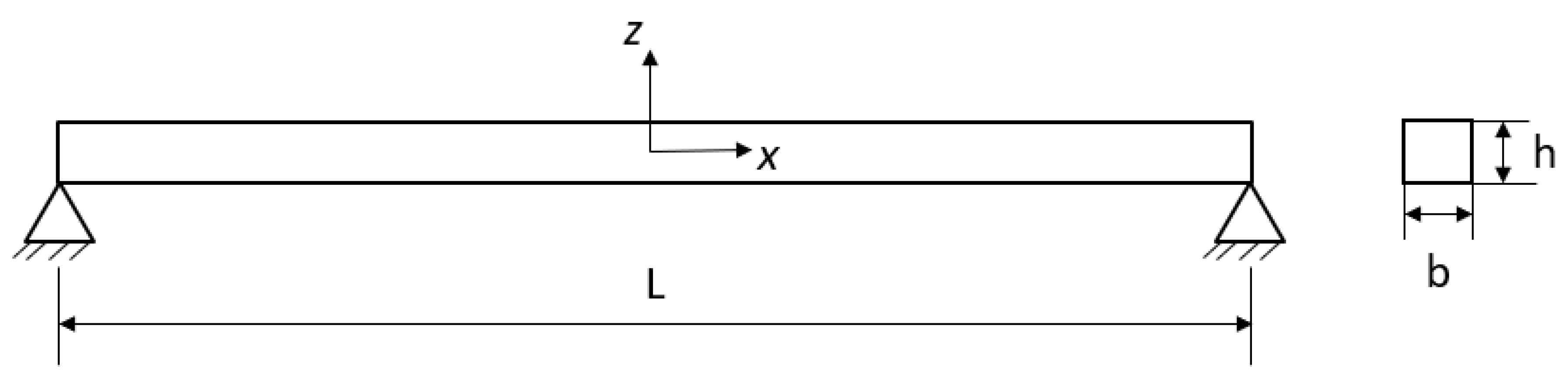
As previously mentioned, this work intends to characterize the free vibration behaviour of quadrilateral nanocomposite plates where the effects of different CNT distributions and agglomeration are to be assessed. Finite element models were implemented using FSDT. The quadrilateral plate is represented in Figure 3.
The plates are considered to be simply supported in the four edges, with a = b for the square plate and b/a = 3 for the rectangular plate. The aspect ratio considered between the x-edge and thickness is a/h = 10.
2.2.1. Constitutive Equations
Considering the FSDT, the displacement field is given by [25,26,27]:
where and are the first-order rotations and , , and are the mid-surface displacements in the directions, respectively, and denotes time. The superscript 0 is going to be used to refer to the mid-surface of the plate. The present theory provides five degrees of freedom.
The strain field is given by [25,26,27]:
where , , and are the in-plane normal and shear strain components; and and are transverse shear strains components.
In the context of a small strains approach, which is the one considered in the present work, the strain field relates with the displacements in the following manner:
Yielding to:
where , , and are the in-plane normal and shear stress components; and are transverse shear stress components; and is the shear correction factor associated with the transverse shear stress components, which for this study is assumed to have the typical value of 5/6.
Considering the random orientation of CNTs, the corresponding nanocomposites can be considered as an isotropic material, thus the elastic stiffness coefficients associated to are given as:
2.2.2. Governing Equations of Motion
Hamilton’s principle can be generically stated as [25]:
where is the kinetic energy, is the elastic strain energy, and is the work performed by applied forces. Considering the aim of the present work, the last term will be null, while the kinetic energy and the elastic strain energy are given as:
By carrying out the necessary mathematical manipulations and considering free harmonic vibrations, one achieves for the whole discretized domain the following equilibrium Equation:
where is the global stiffness matrix, is the global mass matrix, is the natural frequencies, and denotes the vibration mode shapes’ vectors associated to the corresponding natural frequencies [25,26,27].
The global stiffness matrix can be expressed as:
where , , , and are stiffness matrices associated to individualized effects, namely due to membrane, bending, membrane-bending coupling, and transverse shear, respectively. The index refers to a generic element and is the total number of elements considered. The stiffness matrices components are determined by the expressions below [26,27]:
where , , and are the extensional stiffness, the bending extensional coupling stiffness, and the bending stiffness matrices, where its components are given by:
where , , and are the strain-displacement coupling matrices of the bending, membrane, and shear of each element, respectively, and have the following constitution for the present shear deformation theory:
These matrices consider that the generalized displacements vector for each node within each element is ordered as follows:
where is the interpolating functions. In the initial phase of the present work, two plate elements were considered: the bi-linear (Q4) and bi-quadratic (Q9) quadrilateral plate elements with 4 and 9 nodes, respectively [26,27], thus leading to the corresponding interpolating functions:
The Jacobian matrix relates the local coordinates ( of a generic element with the global coordinates (x,y):
The global mass matrix cab be written as [27]:
The matrix is the mass matrix associated with a generic element and can be divided into each of the degrees of freedom contributions, namely:
where and are the inertias associated with the translational and the rotational degrees of freedom, respectively, and they are determined by the following equation, where is the mass density of the nanocomposite [25,27]:
3. Results
This section is divided into two sub-sections: a first one devoted to the verification of the developed codes and a subsequent one that addresses the characterization of the free vibrations behaviour and natural modes’ shapes of square and rectangular plates.
3.1. Verification Studies
3.1.1. On the Use of Eshelby–Mori–Tanaka Agglomeration Model
For the present verification study, which concerns the mechanical properties’ estimation for the FG-CNTRC, the EMT agglomeration model proposed by Shi et al. [8] was used. The Hill’s moduli of the CNTs considered for this purpose are listed in Table 2.
The material of the matrix considered in this case has the following elastic properties: , . This study was performed considering the experimental results obtained by Odegard et al. [29], where the material properties of the present materials were tested for different values of volume fraction of the reinforcement.
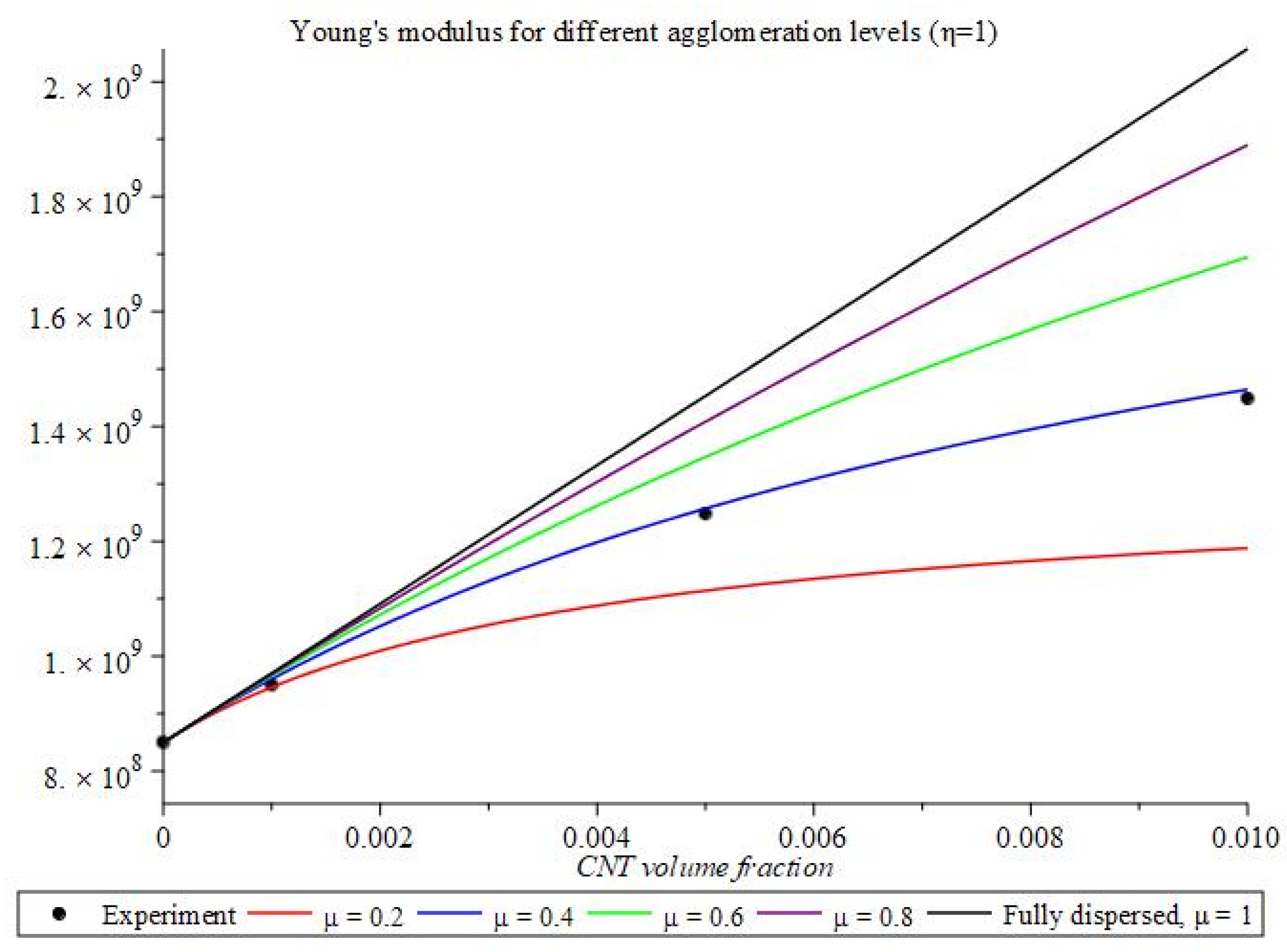
In Figure 4, we observe that the experimental results obtained by Odegard et al. [29] are close to the agglomerated model, where µ = 0.4 as predicted by Barai et al. [13,30] when considering a complete agglomerated model where η=1, meaning that all CNTs are located in inclusions, showing that the employed agglomeration model based on the EMT method is in good agreement with the previous literature (note that the considered points of the experiment led by Odegard et al. were attained through graphic reading and might have slight differences).
Taking the fully dispersed case as a reference, µ = 1, where the Young’s modulus has the higher increase in function of the volume fraction, it is possible to observe that when µ decreases, the increase in the CNT volume fraction does not correspond to the expected increase of mechanical performance due to the severity of the agglomeration effect.
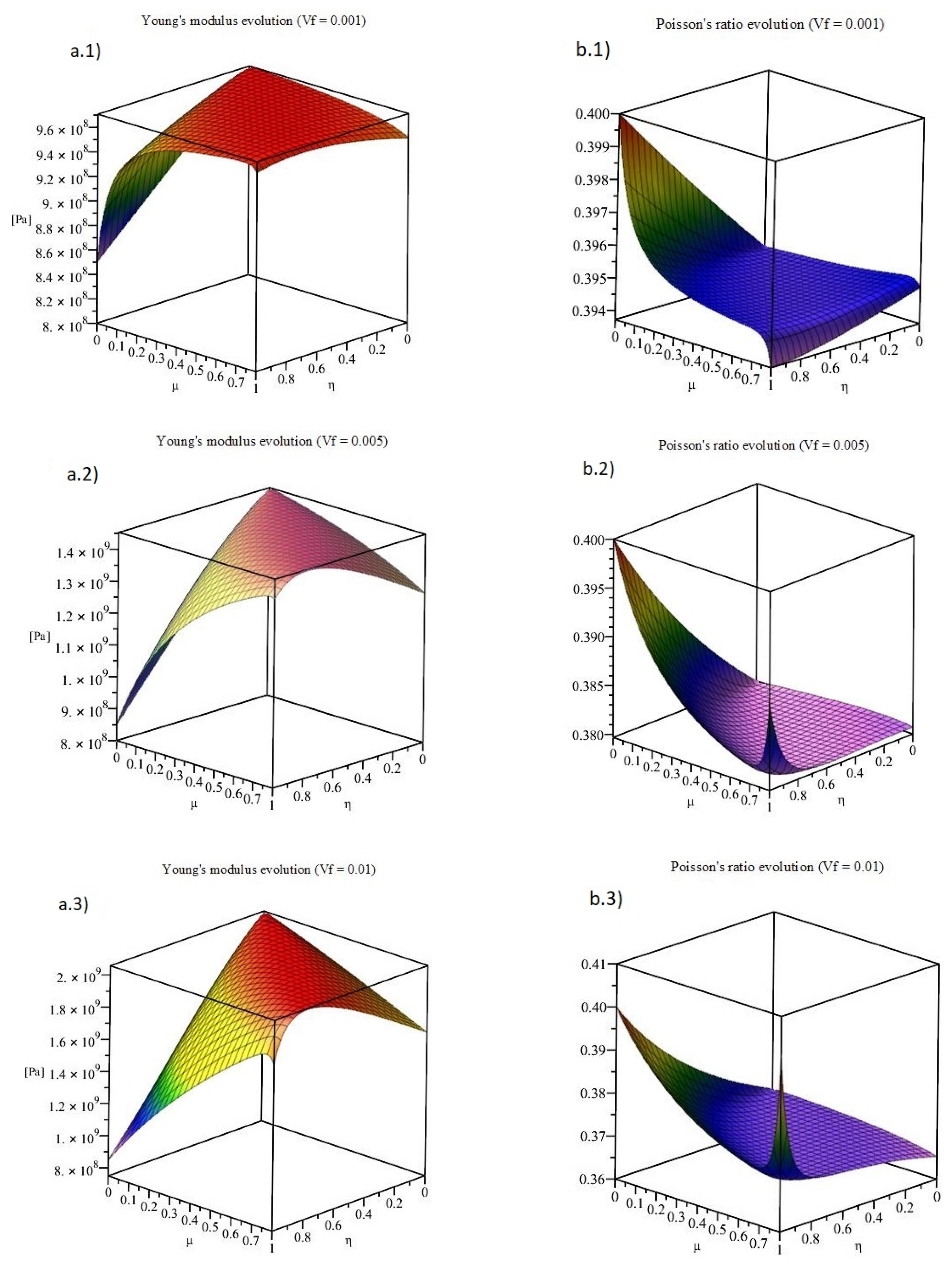
However, partial CNT agglomeration is a more common situation, with this meaning that both parameters η and µ are necessary to describe the agglomeration state [8]. The following graphics represented in Figure 5 show how the Young’s modulus and the Poisson’s ratio behave with the variation of these agglomeration parameters. For this illustration purpose, one considered the CNT volume fractions of 0.1%, 0.5%, and 1%, because they coincide with the points of the experiment led by Odegard et al.
One can observe that the highest values of the Young’ modulus appear when µ = η. It is also possible to observe that the variation of the parameter µ has a higher impact on the elastic properties, when compared to η.
3.1.2. On the Use of FSDT for Free Vibration Analysis
The following verification studies consider a unit length square plate as schematically illustrated in Figure 3 with opposite hinged and simply supported edges in the directions of the plate plane (x,y). Two edge-to-thickness ratios were considered, namely a/h = 10 and a/h = 100.
The material considered for the studies is considered as an isotropic material, and its Poisson’s ratio assumes the value of , and the Young’s modulus and the specific mass and are considered in their SI units [31].
The results are compared in Table 3 with an analytical solution obtained through the Rayleigh–Ritz method for vibration analysis of Mindlin plates [31]. The frequencies are presented in a non-dimensional form using the multiplier:
A convergence study is also presented in the same table.
From Table 3, it is possible to conclude that for both elements, the results are very approximate, if not coincident to the analytic solution, which was expected since the analytic solution presented is for a Mindlin plate. However, one can observe that the element Q9 gives better/faster results even with a smaller number of elements, although the number of degrees of freedom is considerably higher.
Even when comparing the same number of degrees of freedom for the meshes Q4 10 × 10 and Q9 5 × 5 or Q4 20 × 20 and Q9 10 × 10, for example, one can observe a faster convergence for the element Q9, with this happening due the quadratic degree of the interpolating functions that provides a better approximation and thus a better performance for the Q9 plate model.
3.1.3. On the Verification of the FSDT Model for Free Vibration Analysis of an FG-CNTRC Beam Estimated with the EMT Agglomeration Model
The beam was discretized using the Q4 and Q9 plate element models, considering that in the y direction, there is only one element. The natural frequencies convergence study was developed by increasing the number of elements in the x direction.
To allow for the intended verification purpose, the selected beam was the one studied by Yas and Heshmati [5], and it is illustrated in Figure 6. The frequencies are presented in their dimensionless form by considering the multiplier:
where is the area and is the second moment of area of the cross-section of the beam.
The reinforcement material considered in the next verification studies was the SWCNT with a chiral index of (10,10) presented in Table 1, for the matrix phase, the material properties are , , and . The length-to-thickness aspect ratio considered was L/h = 20 and . The length-to-thickness relation, L/b, is equal to 50.
The other authors considered randomly oriented straight CNTs in the matrix, without considering the agglomeration effect. For this purpose, the material properties of the composite were calculated using the EMT agglomeration model using its parameters µ = η, which ensures a uniformly dispersed state of the carbon nanotubes.
To ensure the results of the analysis of the natural frequencies, a convergence study was made considering the distribution UD and using a clamped-clamped (C-C) boundary condition (B.C.). Table 4 presents the results for the bi-linear element Q4 and for the bi-quadric element Q9. The deviations (dev) were calculated as:
In this convergence study, it is observed that using the bi-linear element Q4, the convergence is slower than when using the bi-quadratic element Q9, for the same number of elements. However, the element Q9 has a higher computational cost due to its higher number of nodes per element (nine against four).
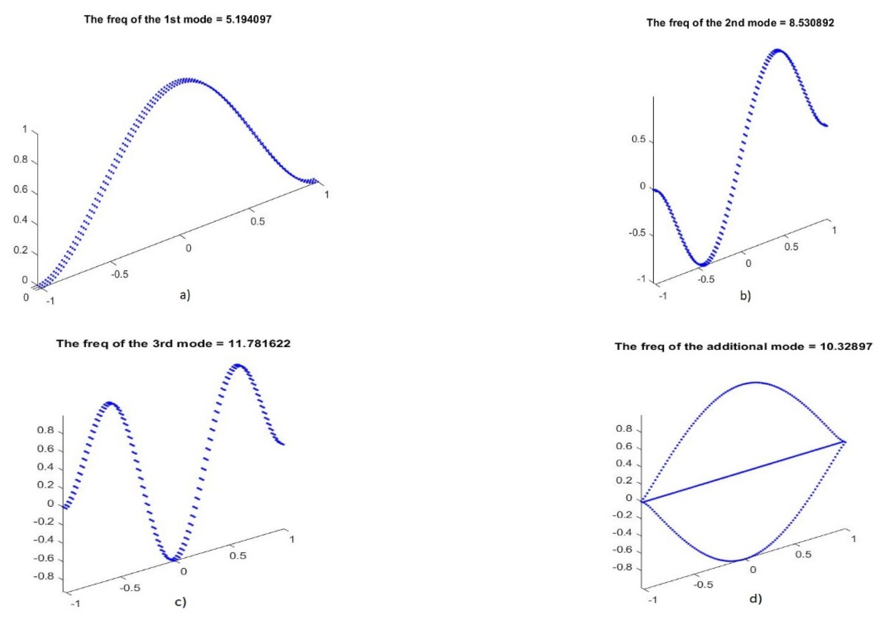
The results of the convergence studies seem to be in reasonable agreement with the results of the considered reference (see [5]) mainly for the first natural frequency. The deviations increase for higher frequencies. These results are expected as one is using 2-D elements, which provide a greater stiffness to the computational model. Additionally, it will be expected that for higher order frequencies, modes that are not expected to appear using Timoshenko beam theory will appear. It is the case of the torsional mode shown in Figure 7.
Additionally, to verify the three CNT volume fraction distributions (UD, USFG, and SFG) and other boundary conditions for the present problem, one performed another study considering the present models to be compared with the Euler Bernoulli beam element and the Timoshenko beam element. In Table 5 and Table 6, where the first three natural frequencies are presented, where one reads H-H, C-F, and C-H, it must be understood as hinged-hinged, clamped-free, and clamped-hinged, respectively.
Despite the convergence study considered until 100 elements, which was the mesh considered by the reference author [5], one has considered a mesh of 50 elements for the next verification with the Q9 element as it provides lower deviations, and also because from 50 to 100 elements, the deviations’ improvement was minimal.
The results presented seem to be in reasonable agreement with the reference, considering that different assumptions are involved when considering a plate and a beam model. The deviations were calculated considering the Timoshenko beam theory as a reference. As expected, they are lower when compared with the Euler–Bernoulli beam results, since the Euler–Bernoulli beam theory does not consider transverse shear components. The present results are higher when compared with the Timoshenko beam theory results, since the 1-D model used to implement it provides a less stiff structure when compared to the 2-D approach considered in the present study.
In this last case, an important trend was identified by Yas and Heshmati [5], in which the frequencies obtained when using the SFG distribution were higher than when using the USFG and the UD, and it was stated that this phenomenon was caused by a better use of the CNTs’ distribution in higher bending stress regions, where they are more concentrated, thus concluding that its bending stiffness was larger than for USFG and UD distributions. In the present study, we can observe the same phenomenon. In this case study, it was also found that there was one more natural frequency between the second and the third natural frequencies considered by Yas and Heshmati [5], which is associated with the natural modes of vibration of a plate. The first four modes of vibration for a UD and (C-C) using the Q9 element type are illustrated in the Figure 7. As expected, the use of a plate model to characterize beams’ natural frequencies is able to provide more information about its modes of vibration.
3.2. Effect of the Agglomeration on FG-CNTRCs Square Plates’ Free Vibrations Behaviour
In the following subsubsections, the free vibrations behaviour of a simply supported square plate as illustrated in the Figure 3 was evaluated using the element Q4 with 20 × 20 elements and Q9 with 15 × 15 elements, where finer meshes were not considered due to its high computational cost and because satisfactory results were obtained with coarser meshes as concluded in Section 3.1.2. The plate’s aspect ratio a/h is equal to 10.
The material of the matrix considered in this study has the following elastic properties: , , and , and the material properties of the reinforcement are listed in Table 2. A value of was considered, as it was found that for a 7.5% concentration, a large amount of CNTs are concentrated in inclusions [23]. The reinforcement distributions considered were the UD, USFD, and the SFD with different levels of agglomeration tested. The dimensionless frequencies to be presented were obtained using the following expression:
3.2.1. Free Vibration Analysis without the Agglomeration Effect
The present study does not consider an agglomerated state, µ = η, and its results serve as a reference for the next ones that consider agglomerated states. For the UD distribution, the results are presented in Table 7.
It is possible to observe that when compared to the other two distributions, the SFG provides the best vibrational characteristics, since its natural frequencies assume higher values. This behaviour is attained because the CNTs are in a higher concentration distributed to higher stress regions.
It is also possible to observe from this table when comparing the results from the Q4 element with the Q9 element, we can see that the frequencies tend to be higher for the Q4 element, which correspond to the expected behaviour.
The next figures present the plots corresponding to the results obtained using only the Q9 plate element, since the results with the Q4 element were similar and the slight differences in the natural frequencies do not interfere with the modes’ shape.
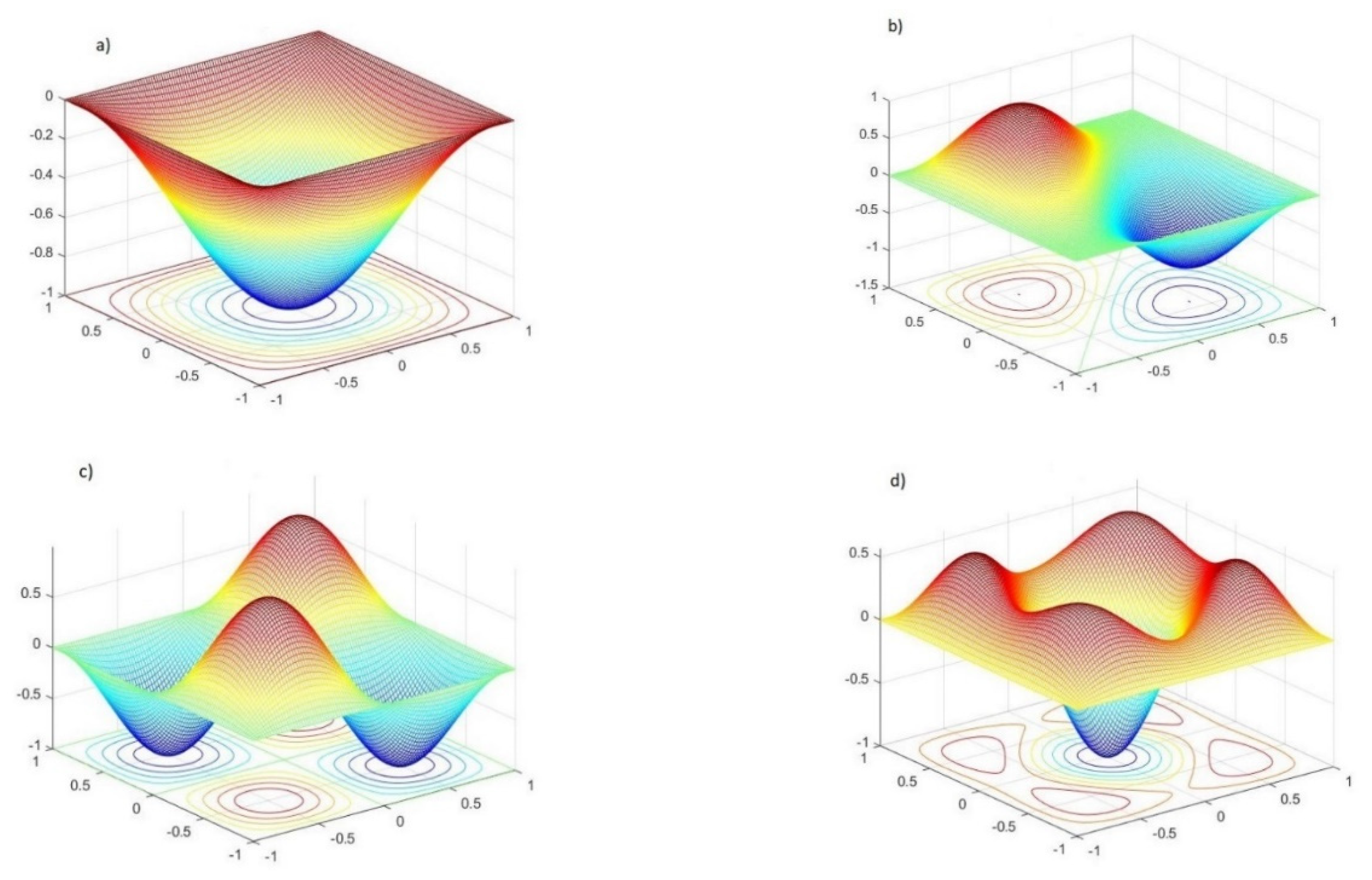
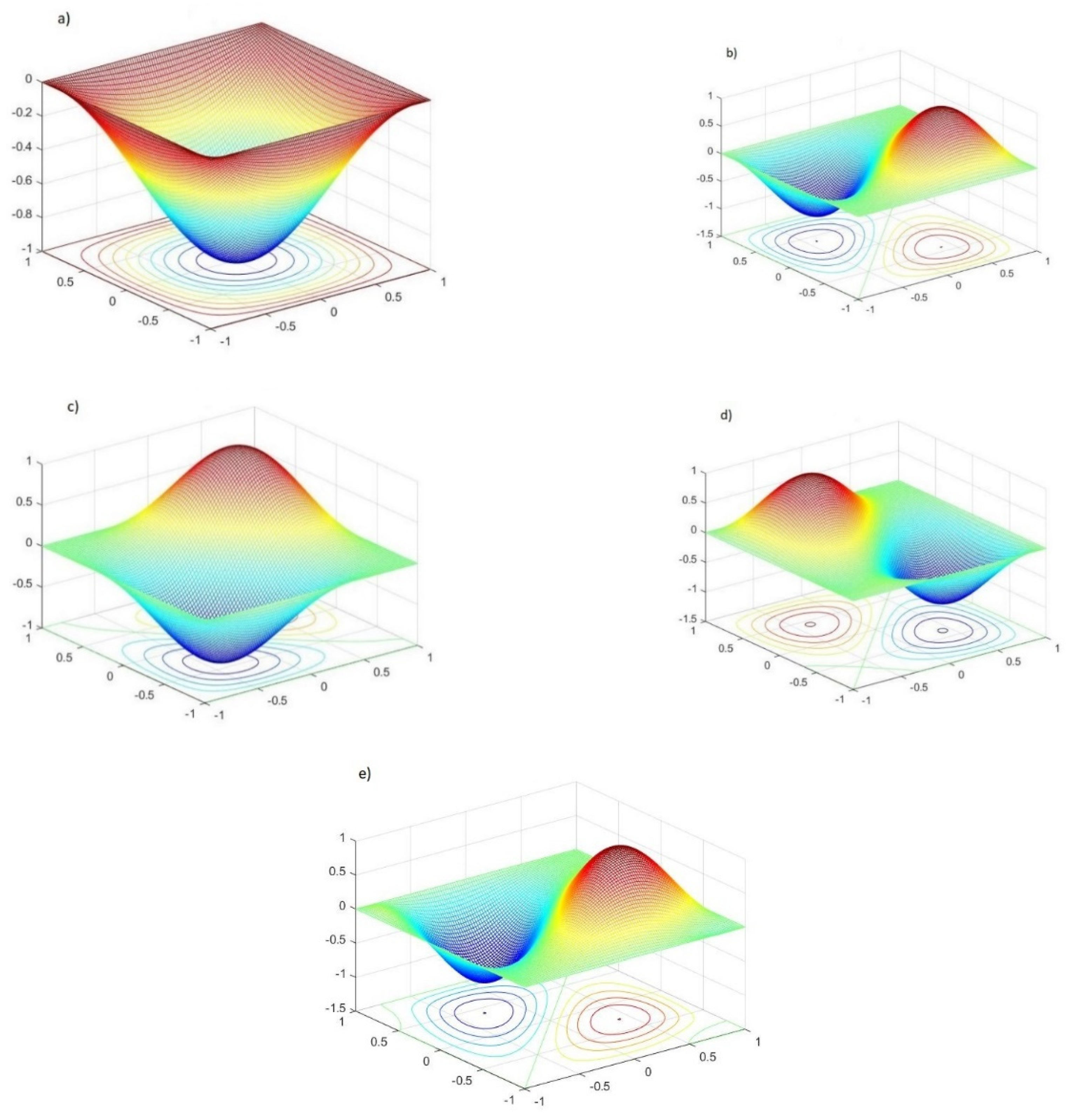
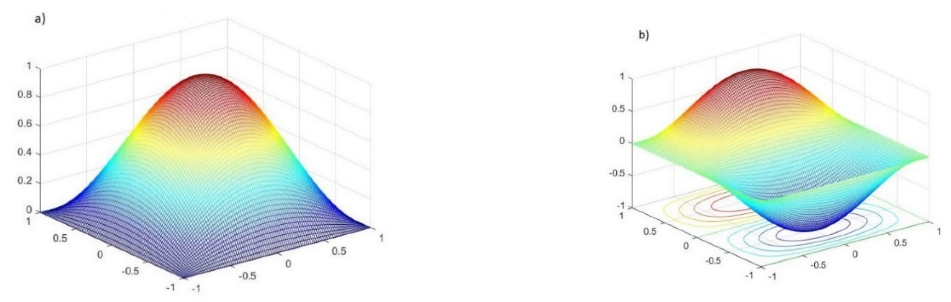
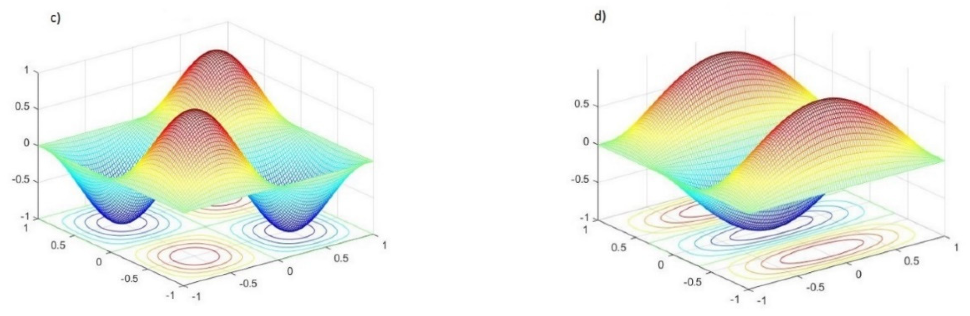
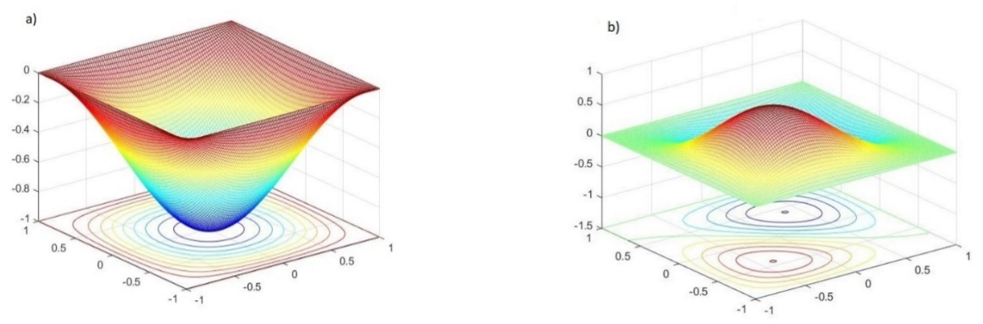
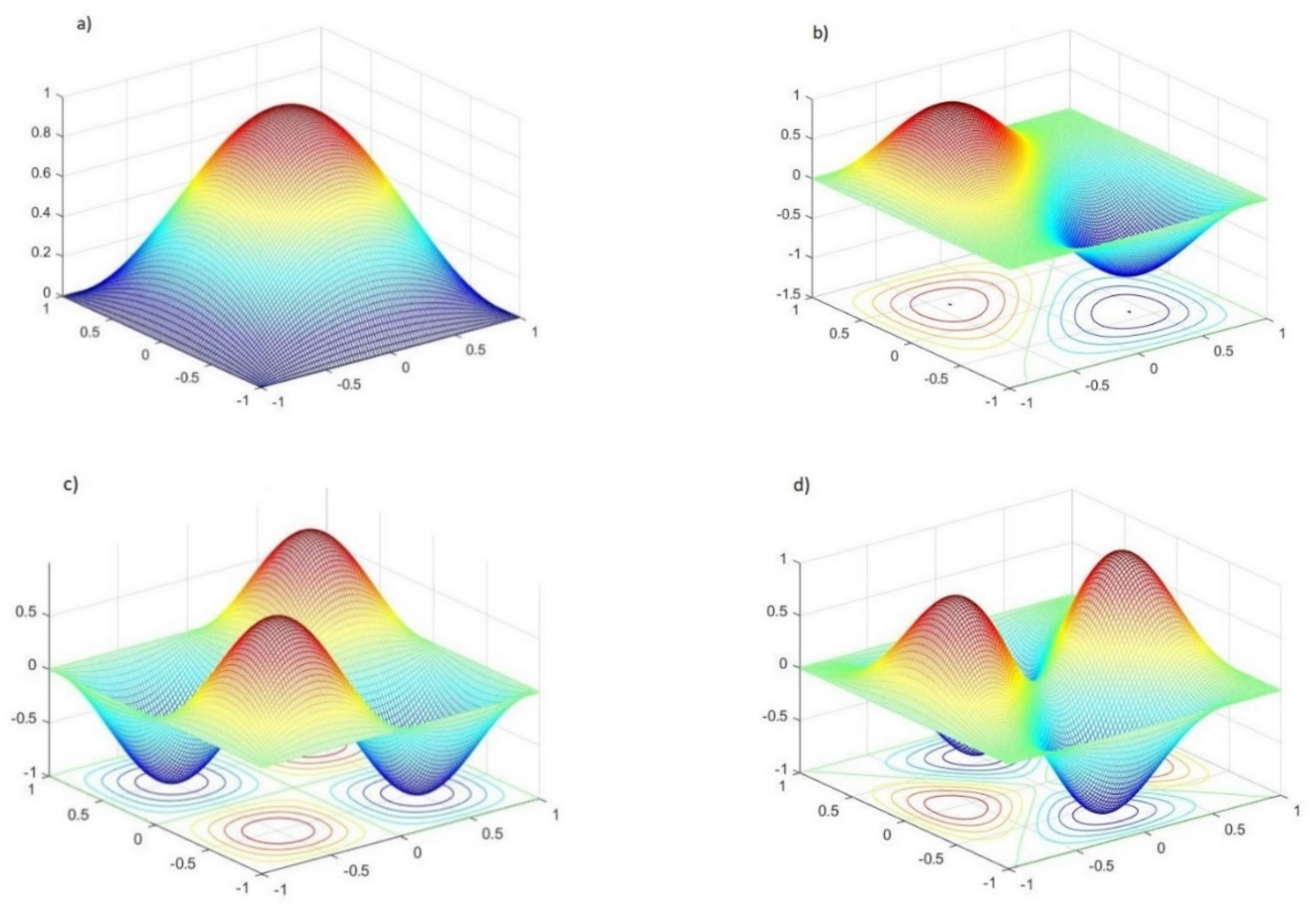
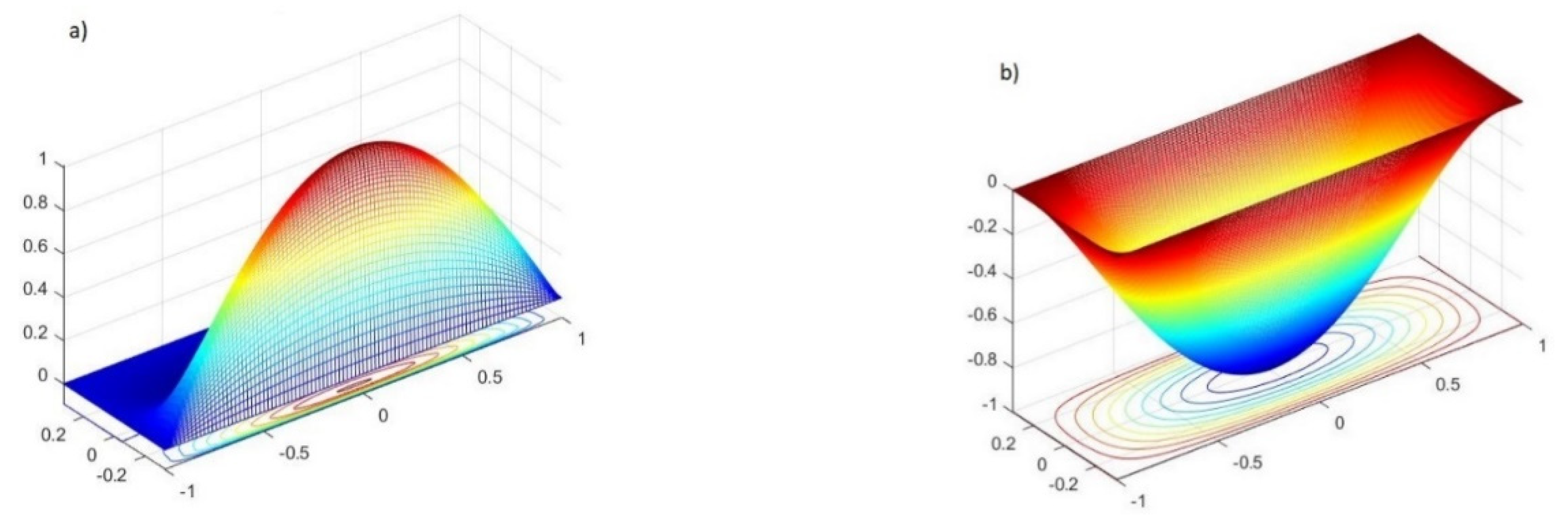
Figure 8 shows the first vibrational modes for the UD distribution of CNTs without the agglomeration effect, noting that the third mode was omitted since it is symmetrical with the second.
From Table 7, one can observe that this distribution has multiple modes, which is due to the symmetries involved in the analysed plate.
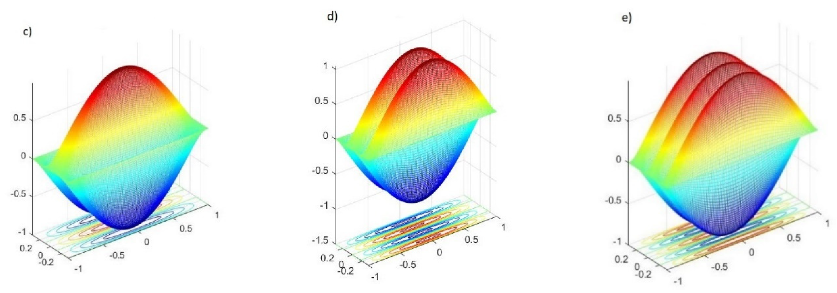
In Figure 9, one can see the first five modes for the USFG distribution. Although some frequencies are close, there is a slight difference that may be due to the CNT asymmetry distribution.
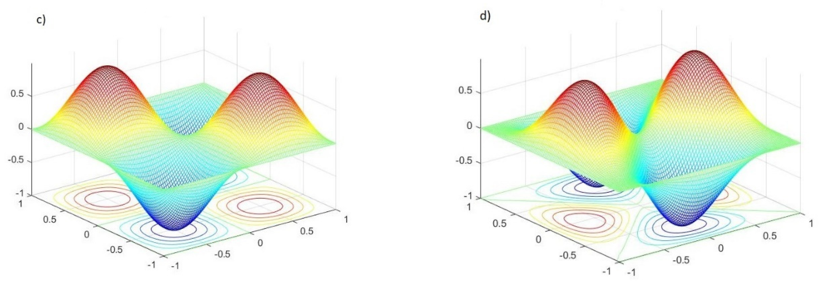
In Figure 10, the first modes for the SFG distribution are illustrated, where the third mode was not displayed since it is symmetrical with the second mode.
Considering the better performance of the biquadratic (Q9) plate model when compared to the bilinear one (Q4), we will only consider Q9 in the next studies.
3.2.2. Free Vibration Analysis for Complete Agglomerated States (η = 1)
This study comprehends a complete state of agglomeration, when η = 1 for three different values of µ = {0.25, 0.5, 0.75}. In these agglomerated states, it is considered that all the CNTs are aggregated in the spherically shaped inclusions [8].
The modes’ shapes for agglomerated states will just be displayed if an observable change on them was identified for any of these three CNT volume fraction distributions.
The results presented in Table 8 are associated to the UD distribution.
From the three states of agglomeration considered, it is possible to observe that the worse vibrational behaviour is precisely when μ = 0.25, which corresponds to the most heterogeneous distribution of CNTs and where the level of agglomeration is more severe.
As it was foreseen in Section 3.1.1, the bigger the difference between the values of the agglomeration parameters, the more its elastic properties would be affected by the agglomeration of the CNTs.
The differences between the natural frequencies are very significant, when comparing these two states of complete agglomeration. When comparing these same frequencies with the ones obtained for a non-agglomerated state in Section 3.2.1, the difference is even higher. Although, the agglomeration effect seems to not interfere with the modes’ shape for this distribution of CNTs along the thickness.
The natural frequencies obtained for the three cases of complete agglomeration considering the USFG distribution are listed in Table 9. From this table, one can conclude that for all cases of complete agglomeration studied, the USFG is the CNT distribution that has the worse dynamic behaviour, when comparing it with the same states of agglomeration for the other CNT distributions.
Similarly to the previous case, the complete agglomerated situations for the USFG CNT volume fraction distribution seem not to interfere significantly with the natural modes’ shape for this distribution.
For the SFG distribution (Table 10), one can observe that, as predicted, the lower the value of the parameter μ, the lower the natural frequencies, just like for the previous distributions.
The modes’ shapes for the SFG distribution are presented in Figure 11 for the severest case of complete agglomeration and in Figure 12 for the least severe case of complete agglomeration studied. The intermediate case is not displayed, since it has the same behaviour as the other cases. For these three cases of complete agglomeration, it is possible to observe a significant change of the fifth mode’s shape, when compared with the non-agglomerated case. For the other three modes’ shapes, no significant changes were observed.
Globally, one can say that for a completely agglomerated case, the more heterogeneous the distribution, the lower the natural frequencies will be for the three CNT distributions studied.
It is also possible to conclude that besides the level of agglomeration, the SFG distribution shows a better vibrational behaviour due to its distribution of CNTs in higher bending stress areas; however, the lesser the value of μ, the lower the differences of the natural frequencies become between distributions.
3.2.3. Free Vibration Analysis for Partially Agglomerated States
In a more general situation, one has situations that are distinct from the completely non-agglomerated state or from the completely agglomerated state, hence being very important to achieve a plausible description of the degree of agglomeration through the parameters µ and η [8].
To investigate the free vibrations’ behaviour of simply supported FG-CNTRC square plates, two different partially agglomerated situations were evaluated, one with η < µ and the other with η > µ, when μ = 0.5 for both situations.
Table 11 presents the first five natural frequencies for the UD distribution.
From this table, when comparing the two states of partial agglomeration, the best free vibration behaviour is achieved with μ = 0.5 and η = 0.25, which corresponds to a state where there is less volume fraction of CNTs in agglomerated inclusions, when compared with μ = 0.5 and η = 0.75.
Although significant differences were found for the natural frequencies when comparing both states of agglomeration, and when comparing these agglomerated states with the results obtained in Section 3.2.1 for a non-agglomerated state, the natural modes’ shapes do not suffer much influence from the agglomeration effect, for these two partially agglomerated states.
In Table 12, one presents the first five natural frequencies for the USFG distribution. In this case the highest natural frequencies appear for η = 0.25, and once again the lesser the volume of CNTs inside the agglomerated inclusions, the better the dynamic free vibrations’ behaviour obtained in the CNTRC.
It was observed that the natural modes’ shapes remained unchanged despite the agglomeration effect when compared to the results obtained for the non-agglomerated state in Section 3.2.1, for the USFG distribution.
Table 13 presents the first five natural frequencies for the SFG distribution. It was also observed in this case that the highest natural frequencies appear for η = 0.25, which translates into a better vibrational behaviour.
For this last distribution, it was observed that the modes’ shape remained unchanged despite the agglomeration effect, for these two cases of partial CNTs agglomeration. The fifth mode change, when in complete agglomeration, may indicate that the more severe the agglomeration, the more prone the interference in the modes’ shapes.
3.3. Effect of the Agglomeration on FG-CNTRCs Rectangular Plates’ Free Vibration Behaviour
In the present case study, the free vibration behaviour of a simply supported rectangular plate was explored under the influence of the agglomeration of CNTs for three different distributions along the thickness direction. The plate is illustrated in Figure 3, with the aspect ratios of a/h = 10 and a/b = 3. The dimensionless results were obtained according to Equation (54), as done in Section 3.2.
3.3.1. Free Vibration Analysis without the Agglomeration Effect
The present study does not consider an agglomerated state, µ = η, in order to consider the achieved results as a reference for the next one, which will consider agglomerated states. Since here it is considered that there is no influence of the agglomeration effect, this study illustrates the best free vibrations’ performance of these rectangular FG-CNTRC plates.
The natural frequencies are presented in Table 14. As expected, one observes that there are no multiple modes for any of the distributions considered, with this happening due to the symmetry loss.
It is also possible to say that for the rectangular plate, the tendency of the SFG distribution having the higher natural frequencies is maintained followed by the UD distribution and at last the USFG distribution with the poorest dynamic behaviour. This results from the distribution of CNTs along the thickness direction, as the higher the concentration of CNTs in high bending stress areas, the higher the natural frequencies.
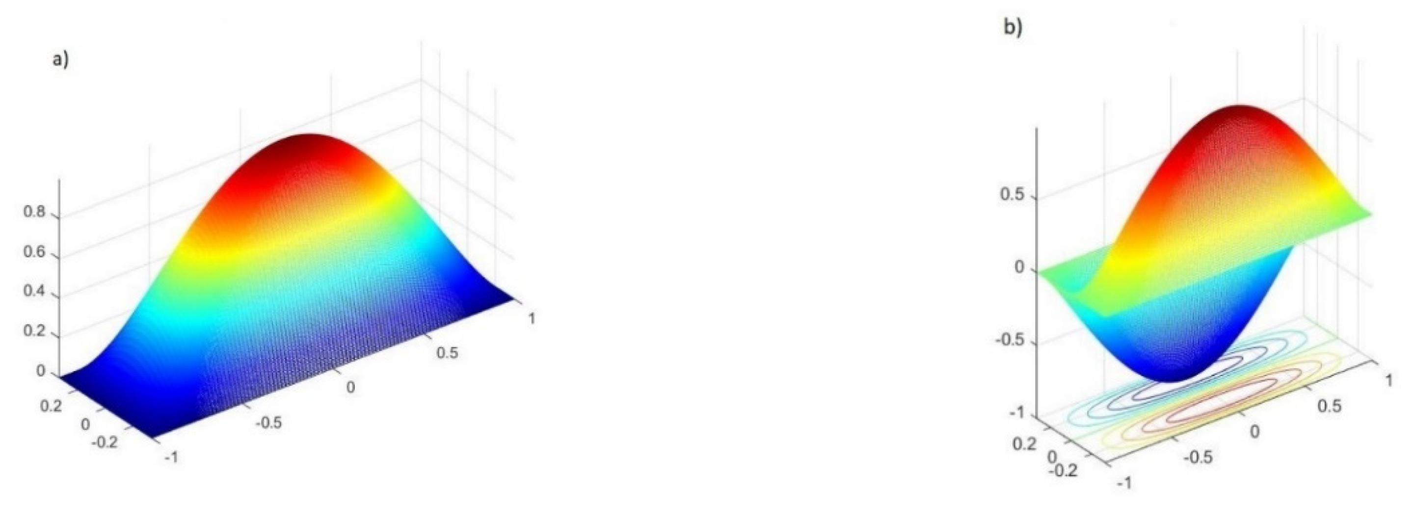
Figure 13 shows the natural modes’ shape without the influence of the CNTs’ agglomeration for the UD distribution.
Figure 14 shows the natural modes’ shape without the influence of the CNTs’ agglomeration for the USFG distribution.
Figure 15 shows the natural modes’ shape without the influence of the CNTs’ agglomeration for the SFG distribution.
3.3.2. Free Vibration Analysis for Complete Agglomerated States (η = 1)
Similarly to the squared plate, for the rectangular plate, the same three states of complete agglomeration, when η = 1 for three different values of µ = {0.25, 0.5, 0.75}, were also considered.
The results listed in Table 15 correspond to the UD distribution. The free vibrations’ behaviour of the rectangular plate tends to worsen with the increase of the severity of the complete agglomerated state, showing lower natural frequencies with the decrease of the parameter μ.
For this case, one can observe that the agglomeration effect exerts influence in the values of the natural frequencies, although the natural modes’ shape seems to be unchanged when comparing to the shapes presented in Section 3.3.1 for the non-agglomerated state for this distribution.
For the USFG distribution, the results for the natural frequencies obtained for the three cases of complete agglomeration can be observed in Table 16. From this table, one can conclude that for all cases of complete agglomeration studied, the USFG is the distribution that has the worse dynamic behaviour for the rectangular plate, when compared with the same states of complete agglomeration for the other CNT distributions.
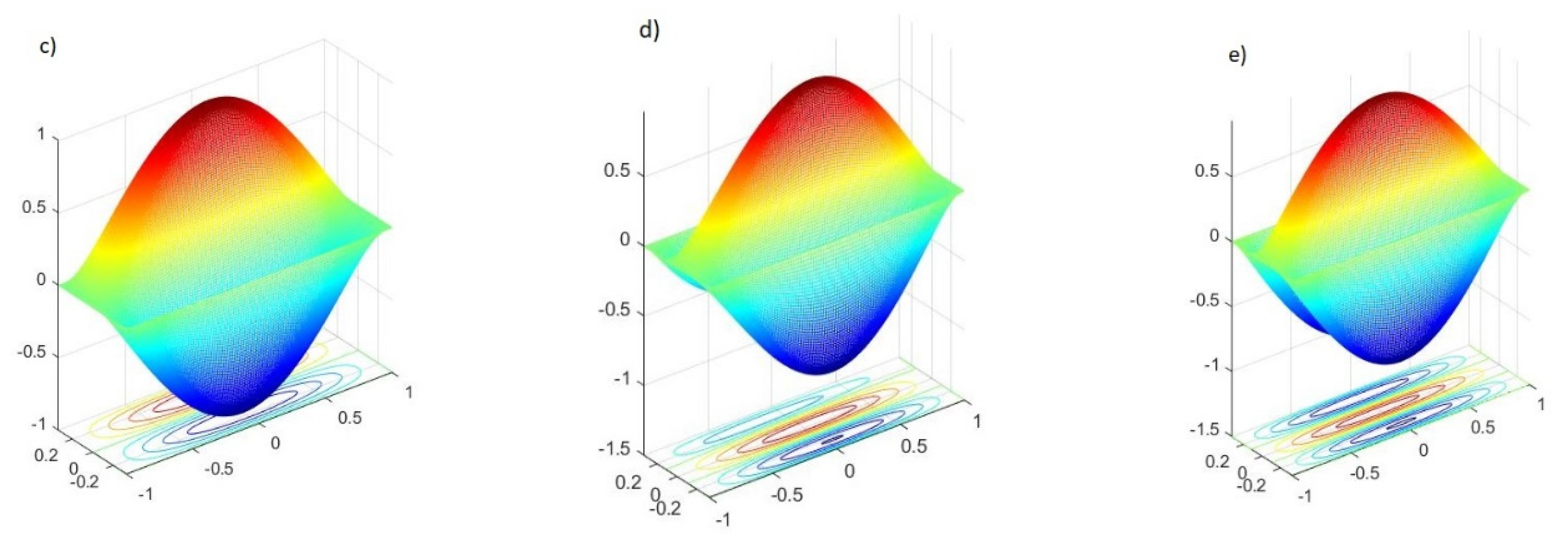
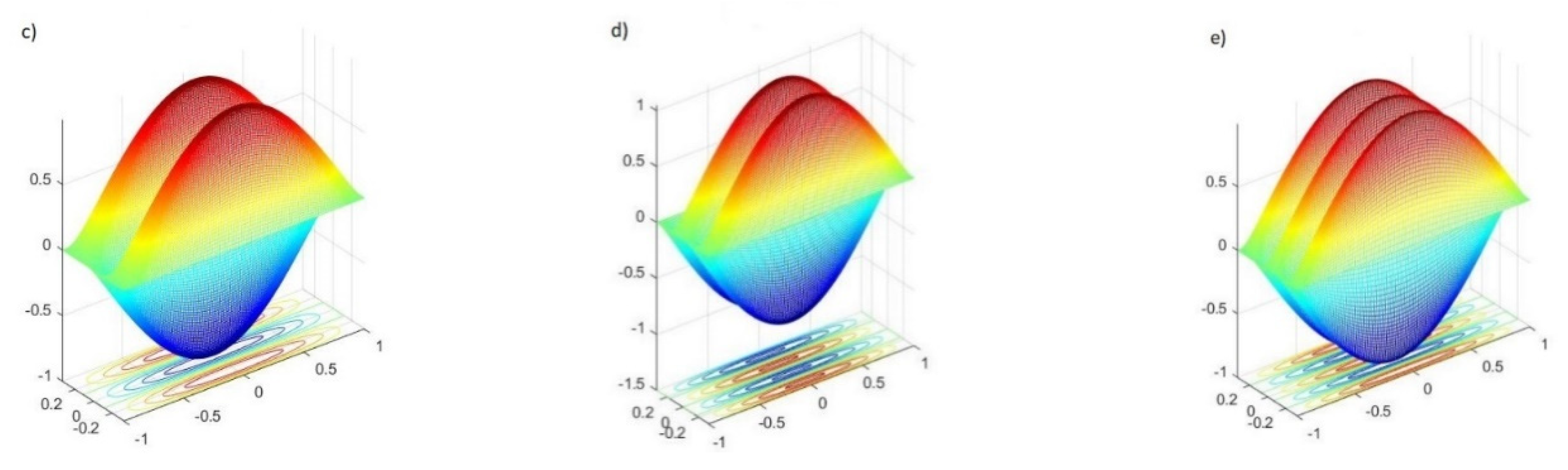
The modes’ shapes for the USFG distribution are presented in Figure 16 for the most severe case of complete agglomeration and in Figure 17 for the intermediate case of complete agglomeration studied. For this distribution, it is possible to see that the agglomeration effect, besides decreasing the natural frequencies, also changes the shapes of the natural modes in some cases, namely the fourth and the fifth mode of the USFG using η = 1 and μ = 0.25, and in the fifth mode when η = 1 and μ = 0.5, when compared with the non-agglomerated state presented in Section 3.3.1. These differences are apparently intensified with the agglomeration state, since for the least severe case, no differences were observed; for the intermediate situation, a difference in the fifth mode was observed; and at last, for the severest situation of complete agglomeration, differences in the fourth and fifth mode were observed.
For the SFG distribution (Table 17), one can observe that, as predicted, the lower the value of the parameter μ, the lower are the natural frequencies, just like for the previous distributions. Once again, the best dynamic behaviour seems to prevail for this distribution regardless of the agglomeration effect when compared with the same agglomeration states for the USFG and UD distributions.
For this distribution, one can observe that the agglomeration effect has a high impact on the natural frequencies, just like for the other distributions. However, the natural modes’ shape did not present significant differences when compared to the non-agglomerated situation.
3.3.3. Free Vibration Analysis for Partially Agglomerated States
Similarly to the study developed for the square plate, the free vibrations’ behaviour of simply supported FG-CNTRC rectangular plates, under different partially agglomerated situations were evaluated, one with η < µ and the other with η > µ, when μ = 0.5 for both situations. As already mentioned, partial agglomeration is more common than complete agglomeration in CNTRC.
In Table 18, we present the first five natural frequencies for the UD distribution.
For this CNTs’ distribution, when comparing the two states of partial agglomeration, the best behaviour found is achieved with μ = 0.5 and η = 0.25, which corresponds to a state where there is less volume fraction of CNTs located in agglomerated inclusions, when compared with μ = 0.5 and η = 0.75.
Significant differences are presented for the natural frequencies when comparing both states of agglomeration, and when comparing these agglomerated states with the results obtained in Section 3.3.1 for a non-agglomerated state. However, in terms of the natural modes’ shapes, no significant differences were found for this partially agglomerated situation when compared with the non-agglomerated state.
Table 19 presents the first five natural frequencies for the USFG distribution. For the rectangular plate with the USFG distribution, the tendency for the highest natural frequencies to appear for η = 0.25 is maintained, and once again, the lesser the volume of CNTs inside the agglomerated inclusions, the better the dynamic behaviour of the plate.
For these two situations of partial agglomeration, when comparing the modes’ shapes results with the ones for a non-agglomerated state (Section 3.3.1), no significant differences were observed for this CNTs unsymmetrical distribution along the thickness direction, different to the previous results for the complete agglomeration (Section 3.3.2), which is another indicator that a more severe state of agglomeration can be more prone to influencing the natural modes.
Finally, in Table 20, we present the first five natural frequencies for the SFG distribution. For this last vibration analysis, it was observed that this distribution provides the highest natural frequencies, which translates into a better vibrational behaviour, when compared to the other distributions due to its enhanced bending stiffness properties.
When comparing both states of agglomeration, one can say that the best dynamic behaviour is reached for η = 0.25, when there is a lesser volume of agglomerated CNTs’ inclusions.
For this last distribution, one can say that the shape of the natural modes remained unchanged despite the agglomeration effect when compared to the results obtained for the non-agglomerated state in Section 3.3.1; however, as already mentioned, there are significant differences in the values of the natural frequencies.
4. Discussion
From the case studies considered, the element Q9 tends to provide lower natural frequencies when compared to the element Q4, due to its greater ability to describe the plate’s shape kinematics, yielding also to more expressive differences for higher order frequencies.
Considering the results of the free vibrations’ behaviour of the FG-CNTRC quadrilateral plates, one can say:
- Since CNTs tend to agglomerate for relatively low CNT volume fractions, this leads to an important conclusion, namely the one that not taking into account the effect of the CNTs’ agglomeration might mislead into an overestimation of the elastic properties of the CNTRC, thus to a less accurate prediction of structure behaviour.
- For all CNTs’ distribution in non-agglomerated situations, the natural frequencies of these structures were always higher when compared with the results for the same CNT distribution if under an agglomerated condition whether it would be a complete or a partial one.
- For all cases considered, i.e., no agglomeration, three different states of complete agglomeration and the two different states of partial agglomeration, the CNTs’ SFG distribution along the thickness direction provided higher natural frequencies, when comparing to the other two distributions considered for the same state of agglomeration. This happens due to the higher concentration of CNTs in high bending stress regions.
- The results of the complete agglomeration studies also demonstrate that the decrease of the agglomeration parameter μ deteriorates the free vibrations’ behaviour of these structures, leading to lower natural frequencies for all the distributions considered.
- When considering partial agglomeration of the CNTs in the FG-CNTRC plates, it can be concluded that the higher the agglomeration parameter η, the lower the natural frequencies for the CNTs’ distributions considered.
With respect to the natural modes’ shape associated to the different natural frequencies:
- On the FG-CNTRC square plates, no significant differences in the modes’ shapes due to the influence of the agglomeration effect were found for the majority of the cases. However, for the SFG CNTs distribution, the fifth mode was affected for complete agglomeration.
- On the FG-CNTRC rectangular plates, for the SFG and UD CNTs distributions, the natural modes’ shapes seem not to be affected with the agglomeration of CNTs; however, for the USFG distribution, differences in the fourth and fifth modes for the complete agglomerated CNTs were found.
Table 21 summarizes the observed differences in the modes’ shapes considering the parametric studies performed. For the majority of the agglomeration cases studied, the agglomeration effect did not show an influence on the modes’ shape.
For the cases where differences were observed, they appear for higher modes (fourth and fifth) and for situations of complete agglomeration of the CNTs. As for the CNTs’ volume fraction distributions, for the square plate, the observed differences occur in the SFG distribution, while for the rectangular plate, the observed differences appeared in the USFG distribution. This allows the conclusion that depending on the agglomeration state, its influence on the natural modes’ shapes also depend on the geometry of the plate and on the CNTs’ distribution along the thickness.
Author Contributions
Conceptualization, D.S.C. and M.A.R.L.; Data curation, D.S.C.; Formal analysis, M.A.R.L.; Methodology, D.S.C. and M.A.R.L.; Software, D.S.C.; Supervision, M.A.R.L.; Validation, D.S.C.; Writing—original draft, D.S.C.; Writing—review and editing, M.A.R.L. All authors have read and agreed to the published version of the manuscript.
Funding
This research was funded by Project IDMEC, LAETA UIDB/50022/2020.
Acknowledgments
The authors wish to acknowledge the support given by FCT/MEC through Project IDMEC, LAETA UIDB/50022/2020.
Conflicts of Interest
The authors declare no conflict of interest.
References
- Kang, I.; Heung, Y.Y.; Kim, J.H.; Lee, J.W.; Gollapudi, R.; Subramaniam, S.; Narasimhadevara, S.; Hurd, D.; Kirikera, G.R.; Shanov, V.; et al. Introduction to carbon nanotube and nanofiber smart materials. Compos. Part B Eng. 2006, 37, 382–394. [Google Scholar] [CrossRef]
- Dai, H. Carbon nanotubes: Opportunities and challenges. Surf. Sci. 2002, 500, 218–241. [Google Scholar] [CrossRef]
- Aragh, B.S.; Barati, A.N.; Hedayati, H. Eshelby–Mori–Tanaka approach for vibrational behavior of continuously graded carbon nanotube-reinforced cylindrical panels. Compos. Part B Eng. 2012, 43, 1943–1954. [Google Scholar] [CrossRef]
- Aragh, B.S.; Farahani, E.B.; Barati, A.N. Natural frequency analysis of continuously graded carbon nanotube-reinforced cylindrical shells based on third-order shear deformation theory. Math. Mech. Solids 2012, 18, 264–284. [Google Scholar] [CrossRef]
- Yas, M.H.; Heshmati, M. Dynamic analysis of functionally graded nanocomposite beams reinforced by randomly oriented carbon nanotube under the action of moving load. Appl. Math. Model. 2012, 36, 1371–1394. [Google Scholar] [CrossRef] [Green Version]
- Shaffer, M.S.P.; Windle, A.H. Fabrication and characterization of carbon nanotube/poly(vinyl alcohol) composites. Adv. Mater. 1999, 11, 937–941. [Google Scholar] [CrossRef]
- Thess, A.; Lee, R.; Nikolaev, P.; Dai, H.; Petit, P.; Robert, J.; Xu, C.; Lee, Y.H.; Kim, S.G.; Rinzler, A.G.; et al. Crystalline Ropes of Metallic Carbon Nanotubes. Science 1996, 273, 483–487. [Google Scholar] [CrossRef] [Green Version]
- Shi, D.-L.; Feng, X.-Q.; Huang, Y.Y.; Hwang, K.-C.; Gao, H. The Effect of Nanotube Waviness and Agglomeration on the Elastic Property of Carbon Nanotube-Reinforced Composites. J. Eng. Mater. Technol. 2004, 126, 250–257. [Google Scholar] [CrossRef]
- Shokrieh, M.; Rafiee, R. Prediction of mechanical properties of an embedded carbon nanotube in polymer matrix based on developing an equivalent long fiber. Mech. Res. Commun. 2010, 37, 235–240. [Google Scholar] [CrossRef]
- Shokrieh, M.; Rafiee, R. On the tensile behavior of an embedded carbon nanotube in polymer matrix with non-bonded interphase region. Compos. Struct. 2010, 92, 647–652. [Google Scholar] [CrossRef]
- He, X.Q.; Eisenberger, M.; Liew, K. The effect of van der Waals interaction modeling on the vibration characteristics of multiwalled carbon nanotubes. J. Appl. Phys. 2006, 100, 124317. [Google Scholar] [CrossRef]
- Strozzi, M.; Pellicano, F. Linear vibrations of triple-walled carbon nanotubes. Math. Mech. Solids 2018, 23, 1456–1481. [Google Scholar] [CrossRef]
- Kamarian, S.; Shakeri, M.; Yas, M.; Bodaghi, M.; Pourasghar, A. Free vibration analysis of functionally graded nanocomposite sandwich beams resting on Pasternak foundation by considering the agglomeration effect of CNTs. J. Sandw. Struct. Mater. 2015, 17, 632–665. [Google Scholar] [CrossRef]
- Heshmati, M.; Yas, M.H. Free vibration analysis of functionally graded CNT-reinforced nanocomposite beam using Eshelby-Mori-Tanaka approach. J. Mech. Sci. Technol. 2013, 27, 3403–3408. [Google Scholar] [CrossRef]
- Kamarian, S.; Salim, M.; Dimitri, R.; Tornabene, F. Free vibration analysis of conical shells reinforced with agglomerated Carbon Nanotubes. Int. J. Mech. Sci. 2016, 108–109, 157–165. [Google Scholar] [CrossRef]
- Tornabene, F.; Fantuzzi, N.; Bacciocchi, M.; Viola, E. Effect of agglomeration on the natural frequencies of functionally graded carbon nanotube-reinforced laminated composite doubly-curved shells. Compos. Part B Eng. 2016, 89, 187–218. [Google Scholar] [CrossRef]
- Tornabene, F.; Fantuzzi, N.; Bacciocchi, M. Linear static response of nanocomposite plates and shells reinforced by agglomerated carbon nanotubes. Compos. Part B Eng. 2017, 115, 449–476. [Google Scholar] [CrossRef]
- Daghigh, H.; Daghigh, V.; Milani, A.; Tannant, D.; Lacy, T.E.; Reddy, J. Nonlocal bending and buckling of agglomerated CNT-reinforced composite nanoplates. Compos. Part B Eng. 2020, 183, 107716. [Google Scholar] [CrossRef]
- Daghigh, V.; Daghigh, V. Free vibration of size and temperature-dependent carbon nanotube (CNT)-reinforced composite nanoplates with CNT agglomeration. Polym. Compos. 2018, 40, 1479–1494. [Google Scholar] [CrossRef]
- Bisheh, H.; Rabczuk, T.; Wu, N. Effects of nanotube agglomeration on wave dynamics of carbon nanotube-reinforced piezocomposite cylindrical shells. Compos. Part B Eng. 2020, 187, 107739. [Google Scholar] [CrossRef]
- Moradi-Dastjerdi, R.; Behdinan, K.; Safaei, B.; Qin, Z. Static performance of agglomerated CNT-reinforced porous plates bonded with piezoceramic faces. Int. J. Mech. Sci. 2020, 188, 105966. [Google Scholar] [CrossRef]
- Krishnaswamy, J.A.; Buroni, F.C.; Garcia-Sanchez, F.; Melnik, R.; Rodriguez-Tembleque, L.; Saez, A. Lead-free piezocomposites with CNT-modified matrices: Accounting for agglomerations and molecular defects. Compos. Struct. 2019, 224, 111033. [Google Scholar] [CrossRef]
- Stéphan, C.; Nguyen, T.; De La Chapelle, M.; Lefrant, S.; Journet, C.; Bernier, P. Characterization of singlewalled carbon nanotubes—PMMA composites. Synth. Met. 2000, 108, 139–149. [Google Scholar] [CrossRef]
- Loja, M.A.R.; Barbosa, J.; Soares, C.M.M. A study on the modeling of sandwich functionally graded particulate composites. Compos. Struct. 2012, 94, 2209–2217. [Google Scholar] [CrossRef] [Green Version]
- Bernardo, G.M.S.; Damásio, F.R.; Silva, T.A.N.; Loja, M.A.R. A study on the structural behaviour of FGM plates: Static and free vibrations analyses. Compos. Struct. 2016, 136, 124–138. [Google Scholar] [CrossRef]
- Reddy, J.N. An Introduction to the Finite Element Method, 2nd ed.; McGraw-Hill, Inc.: New York, NY, USA, 1988. [Google Scholar]
- Reddy, J.N. Mechanics of Laminated Composite Plates and Shells: Theory and Analysis, 2nd ed.; CRC Press: Boca Raton, FL, USA, 2003. [Google Scholar]
- Shen, L.; Li, J. Transversely isotropic elastic properties of single-walled carbon nanotubes. Phys. Rev. B 2004, 69, 1–10. [Google Scholar] [CrossRef]
- Odegard, G.M. Constitutive modeling of nanotube–reinforced polymer composites. Compos. Sci. Technol. 2003, 63, 1671–1687. [Google Scholar] [CrossRef]
- Barai, P.; Weng, G.J. A theory of plasticity for carbon nanotube reinforced composites. Int. J. Plast. 2011, 27, 539–559. [Google Scholar] [CrossRef]
- Dawe, D. Finite strip models for vibration of mindlin plates. J. Sound Vib. 1978, 59, 441–452. [Google Scholar] [CrossRef]
Figure 1.
Eshelby inclusion model of randomly oriented carbon nanotubes.

Figure 2.
CNTs volume fractions distributions illustration.

Figure 3.
Representation of the quadrilateral plate.

Figure 4.
Young′s modulus for different levels of agglomeration and CNT volume fraction.

Figure 5.
Mechanical properties evolution for partially agglomerated states. (a.1) Young’s modulus for Vf = 0.001, (b.1) Poisson’s ratio for Vf = 0.001, (a.2) Young’s modulus for Vf = 0.005, (b.2) Poisson’s ratio for Vf = 0.005, (a.3) Young’s modulus for Vf = 0.01, (b.3) Poisson’s ratio for Vf = 0.01.

Figure 6.
Beam schematic representation.

Figure 7.
Vibrational modes of the beam: (a) 1st mode, (b) 2nd mode, (c) 3rd mode, (d) an additional mode related to the plate natural modes between the 2nd and the 3rd modes.
Figure 7.
Vibrational modes of the beam: (a) 1st mode, (b) 2nd mode, (c) 3rd mode, (d) an additional mode related to the plate natural modes between the 2nd and the 3rd modes.

Figure 8.
Vibrational modes for UD distribution without the agglomeration effect: (a) 1st mode, (b) 2nd mode, (c) 4th mode, (d) 5th mode.
Figure 8.
Vibrational modes for UD distribution without the agglomeration effect: (a) 1st mode, (b) 2nd mode, (c) 4th mode, (d) 5th mode.

Figure 9.
Vibrational modes for USFG distribution without the agglomeration effect: (a) 1st mode, (b) 2nd mode, (c) 3rd mode, (d) 4th mode, (e) 5th mode.
Figure 9.
Vibrational modes for USFG distribution without the agglomeration effect: (a) 1st mode, (b) 2nd mode, (c) 3rd mode, (d) 4th mode, (e) 5th mode.

Figure 10.
Vibrational modes for SFG distribution without the agglomeration effect: (a) 1st mode, (b) 2nd mode, (c) 4th mode, (d) 5th mode.
Figure 10.
Vibrational modes for SFG distribution without the agglomeration effect: (a) 1st mode, (b) 2nd mode, (c) 4th mode, (d) 5th mode.


Figure 11.
Vibrational modes for the SFG distribution with η = 1 and μ = 0.25: (a) 1st mode, (b) 2nd mode, (c) 4th mode, (d) 5th mode.
Figure 11.
Vibrational modes for the SFG distribution with η = 1 and μ = 0.25: (a) 1st mode, (b) 2nd mode, (c) 4th mode, (d) 5th mode.


Figure 12.
Vibrational modes for the SFG distribution with η = 1 and μ = 0.75: (a) 1st mode, (b) 2nd mode, (c) 4th mode, (d) 5th mode.
Figure 12.
Vibrational modes for the SFG distribution with η = 1 and μ = 0.75: (a) 1st mode, (b) 2nd mode, (c) 4th mode, (d) 5th mode.

Figure 13.
Vibrational modes for the UD distribution without the agglomeration effect: (a) 1st mode, (b) 2nd mode, (c) 3rd mode, (d) 4th mode, (e) 5th mode.
Figure 13.
Vibrational modes for the UD distribution without the agglomeration effect: (a) 1st mode, (b) 2nd mode, (c) 3rd mode, (d) 4th mode, (e) 5th mode.


Figure 14.
Vibrational modes for the USFG distribution without the agglomeration effect: (a) 1st mode, (b) 2nd mode, (c) 3rd mode, (d) 4th mode, (e) 5th mode.
Figure 14.
Vibrational modes for the USFG distribution without the agglomeration effect: (a) 1st mode, (b) 2nd mode, (c) 3rd mode, (d) 4th mode, (e) 5th mode.
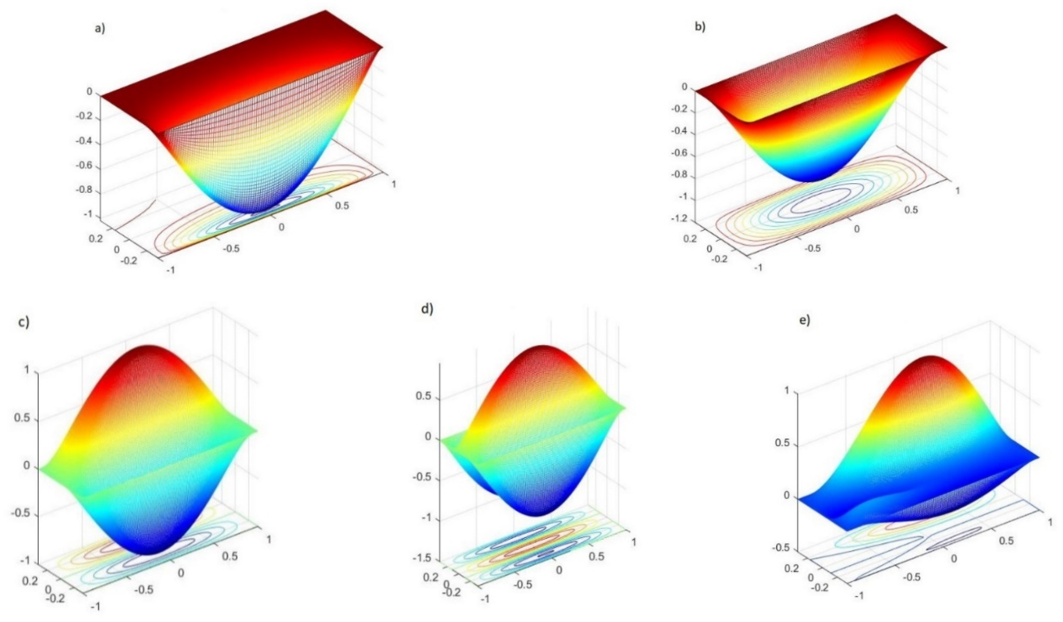
Figure 15.
Vibrational modes for the SFG distribution without the agglomeration effect: (a) 1st mode, (b) 2nd mode, (c) 3rd mode, (d) 4th mode, (e) 5th mode.
Figure 15.
Vibrational modes for the SFG distribution without the agglomeration effect: (a) 1st mode, (b) 2nd mode, (c) 3rd mode, (d) 4th mode, (e) 5th mode.
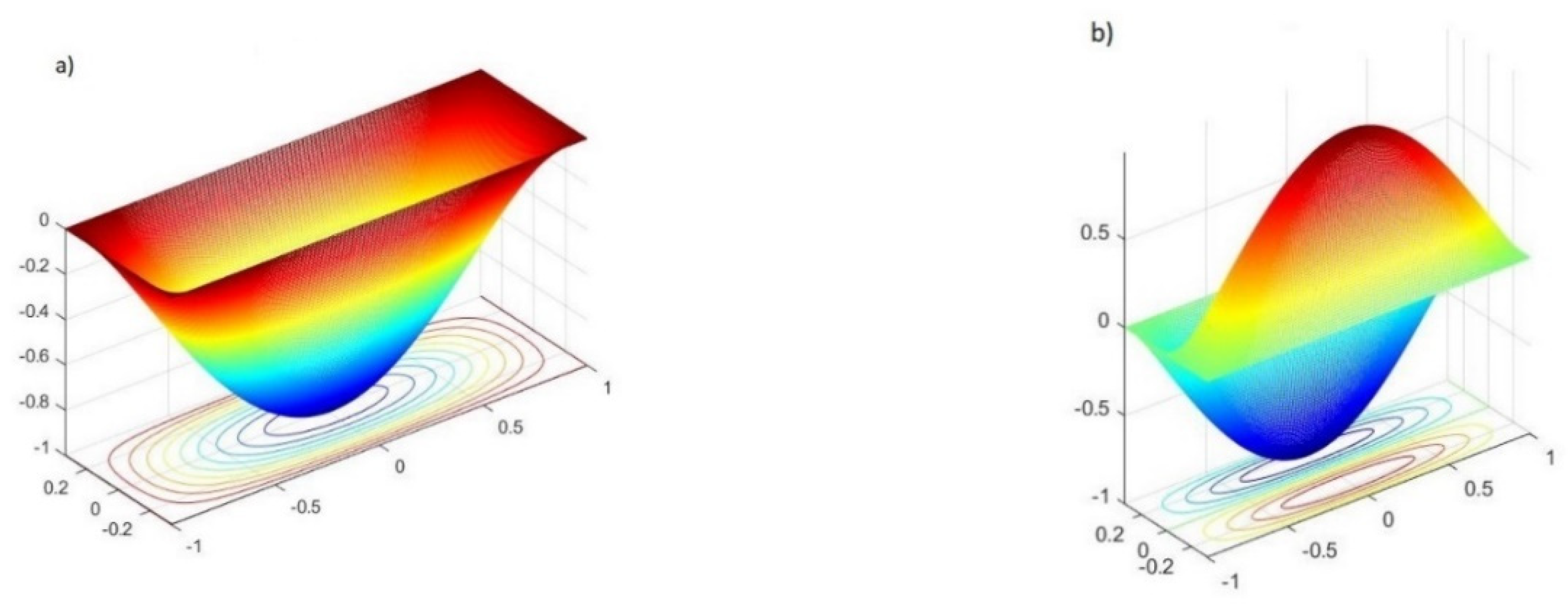

Figure 16.
Vibrational modes for the USFG distribution with η = 1 and μ = 0.25: (a) 1st mode, (b) 2nd mode, (c) 3rd mode, (d) 4th mode, (e) 5th mode.
Figure 16.
Vibrational modes for the USFG distribution with η = 1 and μ = 0.25: (a) 1st mode, (b) 2nd mode, (c) 3rd mode, (d) 4th mode, (e) 5th mode.
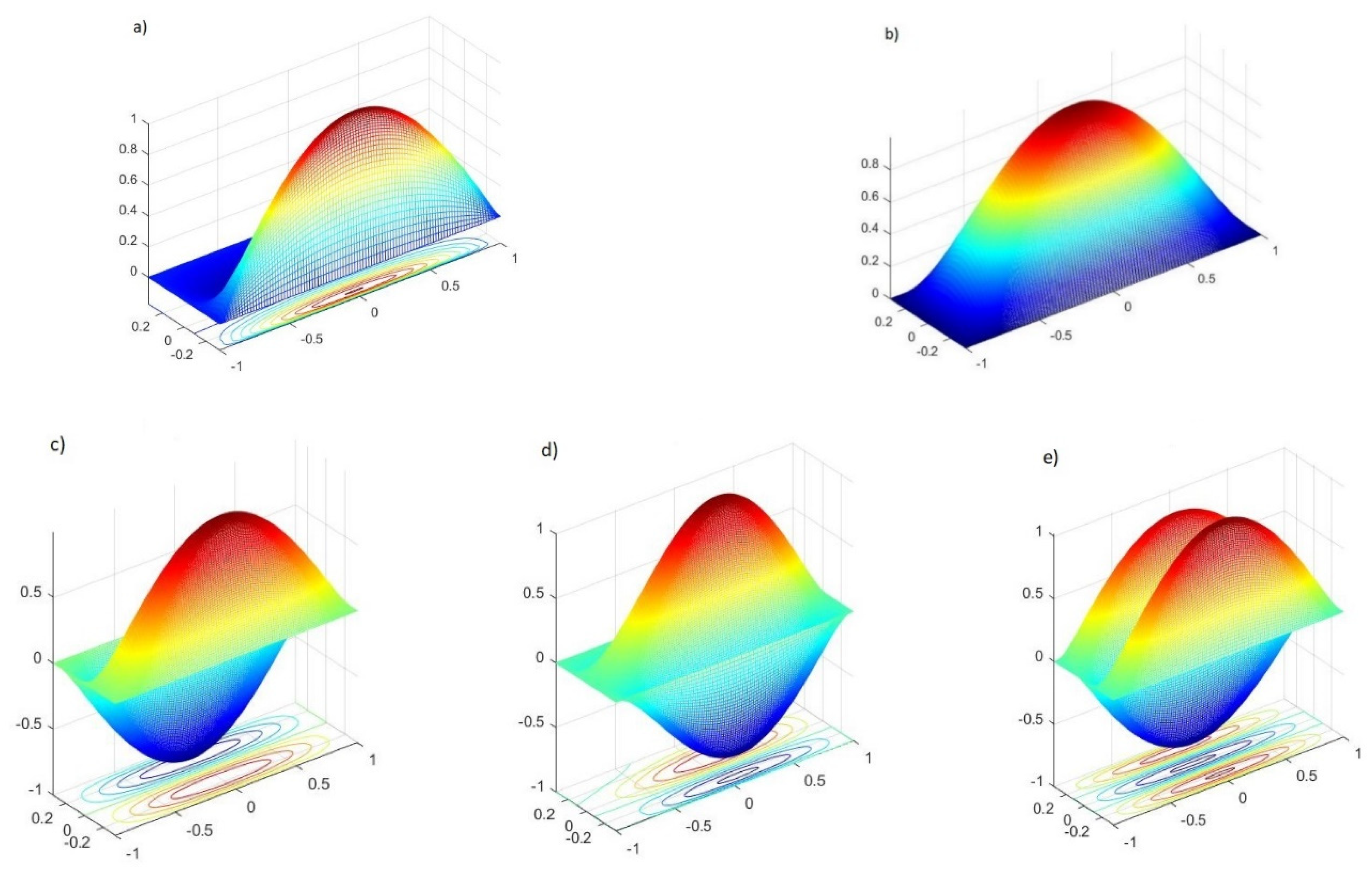
Figure 17.
Vibrational modes for the USFG distribution with η = 1 and μ = 0.5: (a) 1st mode, (b) 2nd mode, (c) 3rd mode, (d) 4th mode, (e) 5th mode.
Figure 17.
Vibrational modes for the USFG distribution with η = 1 and μ = 0.5: (a) 1st mode, (b) 2nd mode, (c) 3rd mode, (d) 4th mode, (e) 5th mode.


Table 1.
Properties of the equivalent fibre for SWCNT (10,10) [10].
Table 1.
Properties of the equivalent fibre for SWCNT (10,10) [10].
| Equivalent Fibre | |
|---|---|
| Longitudinal elastic modulus (GPa) | 649.12 |
| Transverse elastic modulus (GPa) | 11.27 |
| Transverse shear modulus (GPa) | 5.13 |
| Poisson′s ratio | 0.284 |
| Density (kg/m3) | 1400 |
Table 2.
Hill’s moduli of the SWCNT [28].
Table 2.
Hill’s moduli of the SWCNT [28].
| Hill’s Elastic Moduli (GPa) | |
|---|---|
| 271 | |
| 88 | |
| 17 | |
| 1089 | |
| 442 | |
| Density (kg/m3) | 1400 |
Table 3.
Convergence study for the first natural frequency of a square plate.
| Mesh | a/h = 10 | a/h = 100 | ||||
|---|---|---|---|---|---|---|
| Q4 (DOF) | Q9 (DOF) | Analytic Solution | Q4 (DOF) | Q9 (DOF) | Analytic Solution | |
| 5 × 5 | - | 0.9305 (605) | 0.9300 | - | 0.0963 (605) | 0.0963 |
| 10 × 10 | 0.9399 (605) | 0.9303 (2205) | 0.0973 (605) | 0.0963 (2205) | ||
| 15 × 15 | 0.9346 (1280) | 0.9303 (4805) | 0.0968 (1280) | 0.0963 (4805) | ||
| 20 × 20 | 0.9327 (2205) | - | 0.0965 (2205) | - | ||
| 25 × 25 | 0.9318 (3380) | - | 0.0965 (3380) | - | ||
Table 4.
Convergence analysis using the bi-linear element Q4 and the bi-quadratic element Q9.
| Number of Elements | ||||||
|---|---|---|---|---|---|---|
| λ | 15 | 25 | 50 (dev) | 75 | 100 (dev) | Timoshenko beam [5] |
| Q4 | ||||||
| 1 | 5.24450 | 5.21481 | 5.20024 (1.994) | 5.19698 | 5.19571 (1.905) | 5.098585 |
| 2 | 8.71002 | 8.59864 | 8.54931 (7.757) | 8.53935 | 8.53566 (7.585) | 7.93386 |
| 3 | 12.21564 | 11.93952 | 11.82283 (13.41) | 11.80034 | 11.79223 (13.11) | 10.42527 |
| Total DOF | 160 | 260 | 510 | 760 | 1010 | |
| λ | Q9 | |||||
| 1 | 5.19881 | 5.19589 | 5.19410 (1.873) | 5.19371 | 5.19358 (1.863) | 5.098585 |
| 2 | 8.53882 | 8.53377 | 8.53089 (7.525) | 8.53028 | 8.53008 (7.515) | 7.93386 |
| 3 | 11.79418 | 11.78565 | 11.78162 (13.01) | 11.78080 | 11.78055 (13.00) | 10.42527 |
| Total DOF | 465 | 765 | 1515 | 2265 | 3015 | |
Table 5.
Natural frequencies in order of the material distribution and boundary conditions.
| λ | B. C. | Euler-Bernoulli Beam Element [5] | Timoshenko Beam Element [5] | ||||
|---|---|---|---|---|---|---|---|
| UD | USFG | SFG | UD | USFG | SFG | ||
| 1 | C-C | 5.4647 | 5.3708 | 5.7495 | 5.098585 | 5.031699 | 5.294657 |
| 2 | 9.0571 | 8.9005 | 9.5291 | 7.93386 | 7.85222 | 8.167861 | |
| 3 | 12.6469 | 12.4262 | 13.3056 | 10.42527 | 10.3392 | 10.66974 | |
| 1 | H-H | 3.63 | 3.6182 | 3.8192 | 3.574603 | 3.563695 | 3.748668 |
| 2 | 7.2489 | 7.1216 | 7.6266 | 6.854168 | 6.757675 | 7.133685 | |
| 3 | 10.8457 | 10.6722 | 11.4107 | 9.71082 | 9.610907 | 10.02423 | |
| 1 | C-F | 2.1672 | 2.13 | 2.2802 | 2.151246 | 2.115347 | 2.259759 |
| 2 | 5.4175 | 5.324 | 5.6998 | 5.167211 | 5.09299 | 5.385917 | |
| 3 | 9.0443 | 8.887 | 9.5155 | 8.194459 | 8.096988 | 8.475179 | |
| 1 | C-H | 4.5367 | 4.4696 | 4.7731 | 4.356794 | 4.302608 | 4.546786 |
| 2 | 8.1535 | 8.0173 | 8.5784 | 7.426815 | 7.341066 | 7.685675 | |
| 3 | 11.7464 | 11.5427 | 12.3583 | 10.08701 | 9.991091 | 10.3645 | |
Table 6.
Natural frequencies in order of the material distribution and boundary conditions. Present model with Q9 element.
Table 6.
Natural frequencies in order of the material distribution and boundary conditions. Present model with Q9 element.
| λ | B. C. | Present Model [FSDT] | ||
|---|---|---|---|---|
| UD (dev) | USFG (dev) | SFG (dev) | ||
| 1 | C-C | 5.19410 (1.873) | 5.23446 (4.030) | 5.41031 (2.184) |
| 2 | 8.53089 (7.525) | 8.59440 (9.452) | 8.87200 (8.621) | |
| 3 | 11.78162 (13.01) | 11.86476 (14.75) | 12.23028 (14.63) | |
| 1 | H-H | 3.46974 (2.934) | 3.52617 (1.053) | 3.61832 (3.477) |
| 2 | 6.89656 (0.618) | 6.95265 (2.885) | 7.18576 (0.730) | |
| 3 | 10.24292 (5.479) | 10.33215 (7.504) | 10.65856 (6.328) | |
| 1 | C-F | 2.07402 (3.590) | 2.09119 (1.142) | 2.16316 (4.275) |
| 2 | 5.16153 (0.110) | 5.20323 (2.165) | 5.37898 (0.129) | |
| 3 | 8.55821 (4.439) | 8.62481 (6.519) | 8.90793 (5.106) | |
| 1 | C-H | 4.32579 (0.712) | 4.36675 (1.491) | 4.50872 (0.837) |
| 2 | 7.72167 (3.970) | 7.78485 (6.045) | 8.03845 (4.590) | |
| 3 | 11.02165 (9.266) | 11.10498 (11.15) | 11.45557 (10.53) | |
Table 7.
First five natural frequencies for the FG-CNTRC square plate with different distributions without the agglomeration effect.
Table 7.
First five natural frequencies for the FG-CNTRC square plate with different distributions without the agglomeration effect.
| λ | UD | USFG | SFG | |||
|---|---|---|---|---|---|---|
| Q4 | Q9 | Q4 | Q9 | Q4 | Q9 | |
| 1 | 11.1259 | 11.0975 | 10.2156 | 10.1876 | 13.0043 | 12.9717 |
| 2 | 26.6616 | 26.4300 | 24.0251 | 23.8584 | 30.7728 | 30.5147 |
| 3 | 26.6616 | 26.4300 | 24.3895 | 24.1794 | 30.7728 | 30.5147 |
| 4 | 40.8513 | 40.5000 | 26.0625 | 26.0013 | 46.6761 | 46.2997 |
| 5 | 50.3098 | 49.3144 | 29.7480 | 29.7034 | 57.1369 | 56.0610 |
Table 8.
First five natural frequencies for the UD distribution for three different states of complete agglomeration.
Table 8.
First five natural frequencies for the UD distribution for three different states of complete agglomeration.
| λ | η = 1 μ = 0.25 | η = 1 μ = 0.5 | η = 1 μ = 0.75 |
|---|---|---|---|
| 1 | 7.2119 | 9.8010 | 8.5212 |
| 2 | 17.1866 | 23.3547 | 20.3099 |
| 3 | 17.1866 | 23.3547 | 20.3099 |
| 4 | 26.3491 | 35.8032 | 31.1414 |
| 5 | 32.0929 | 43.6063 | 37.9327 |
Table 9.
First five natural frequencies for the USFG distribution for three different states of complete agglomeration.
Table 9.
First five natural frequencies for the USFG distribution for three different states of complete agglomeration.
| λ | η = 1 μ = 0.25 | η = 1 μ = 0.5 | η = 1 μ = 0.75 |
|---|---|---|---|
| 1 | 6.9518 | 7.9533 | 8.9882 |
| 2 | 16.5096 | 18.8644 | 21.2173 |
| 3 | 16.5822 | 18.9727 | 21.4074 |
| 4 | 16.7036 | 19.5689 | 22.5596 |
| 5 | 19.0766 | 22.3055 | 25.7035 |
Table 10.
First five natural frequencies for the SFG distribution for three different states of complete agglomeration.
Table 10.
First five natural frequencies for the SFG distribution for three different states of complete agglomeration.
| λ | η = 1 μ = 0.25 | η = 1 μ = 0.5 | η = 1 μ = 0.75 |
|---|---|---|---|
| 1 | 7.2801 | 10.6382 | 8.8357 |
| 2 | 17.3136 | 25.1455 | 20.9576 |
| 3 | 17.3136 | 25.1455 | 20.9576 |
| 4 | 26.4997 | 38.2979 | 32.0087 |
| 5 | 32.2457 | 46.4714 | 38.9016 |
Table 11.
First five natural frequencies for the UD distribution for two different states of partial agglomeration.
Table 11.
First five natural frequencies for the UD distribution for two different states of partial agglomeration.
| λ | η = 0.25 μ = 0.5 | η = 0.75 μ = 0.5 |
|---|---|---|
| 1 | 10.7993 | 10.6423 |
| 2 | 25.7258 | 25.3509 |
| 3 | 25.7258 | 25.3509 |
| 4 | 39.4283 | 38.8528 |
| 5 | 48.0147 | 47.3131 |
Table 12.
First five natural frequencies for the USFG distribution for two different states of partial agglomeration.
Table 12.
First five natural frequencies for the USFG distribution for two different states of partial agglomeration.
| λ | η = 0.25 μ = 0.5 | η = 0.75 μ = 0.5 |
|---|---|---|
| 1 | 9.9679 | 9.8321 |
| 2 | 23.3603 | 23.0535 |
| 3 | 23.6652 | 23.3503 |
| 4 | 25.3939 | 24.9567 |
| 5 | 28.9605 | 28.4688 |
Table 13.
First five natural frequencies for the SFG distribution for two different states of partial agglomeration.
Table 13.
First five natural frequencies for the SFG distribution for two different states of partial agglomeration.
| λ | η = 0.25 μ = 0.5 | η = 0.75 μ = 0.5 |
|---|---|---|
| 1 | 12.5694 | 12.2965 |
| 2 | 29.5889 | 28.9567 |
| 3 | 29.5889 | 28.9567 |
| 4 | 44.9194 | 43.9722 |
| 5 | 54.4064 | 53.2675 |
Table 14.
First five natural frequencies for the FG-CNTRC rectangular plate with different distributions without the agglomeration effect.
Table 14.
First five natural frequencies for the FG-CNTRC rectangular plate with different distributions without the agglomeration effect.
| λ | UD | USFG | SFG |
|---|---|---|---|
| 1 | 49.3032 | 29.4880 | 56.0488 |
| 2 | 61.7868 | 45.0712 | 69.7297 |
| 3 | 81.0005 | 56.8115 | 90.5044 |
| 4 | 105.2993 | 74.2900 | 116.3783 |
| 5 | 133.2387 | 76.6857 | 145.6953 |
Table 15.
First five natural frequencies for the UD distribution for three different states of complete agglomeration.
Table 15.
First five natural frequencies for the UD distribution for three different states of complete agglomeration.
| λ | η = 1 μ = 0.25 | η = 1 μ = 0.5 | η = 1 μ = 0.75 |
|---|---|---|---|
| 1 | 32.0856 | 37.9241 | 43.5964 |
| 2 | 40.2250 | 47.5490 | 54.6530 |
| 3 | 52.7614 | 62.3764 | 71.6812 |
| 4 | 68.6291 | 81.1477 | 93.2317 |
| 5 | 86.8894 | 102.7540 | 118.0290 |
Table 16.
First five natural frequencies for the USFG distribution for three different states of complete agglomeration.
Table 16.
First five natural frequencies for the USFG distribution for three different states of complete agglomeration.
| λ | η = 1 μ = 0.25 | η = 1 μ = 0.5 | η = 1 μ = 0.75 |
|---|---|---|---|
| 1 | 19.0417 | 22.2483 | 25.5956 |
| 2 | 31.0008 | 35.5023 | 40.0258 |
| 3 | 38.8980 | 44.6043 | 50.3604 |
| 4 | 49.8835 | 58.2905 | 65.8665 |
| 5 | 50.4338 | 58.3212 | 66.9380 |
Table 17.
First five natural frequencies for the SFG distribution for three different states of complete agglomeration.
Table 17.
First five natural frequencies for the SFG distribution for three different states of complete agglomeration.
| λ | η = 1 μ = 0.25 | η = 1 μ = 0.5 | η = 1 μ = 0.75 |
|---|---|---|---|
| 1 | 32.2384 | 38.8929 | 46.4611 |
| 2 | 40.3660 | 48.6204 | 57.9616 |
| 3 | 52.8553 | 63.5232 | 75.5133 |
| 4 | 68.6205 | 82.2699 | 97.4962 |
| 5 | 86.7151 | 103.7140 | 122.5369 |
Table 18.
First five natural frequencies for the UD distribution for two different states of partial agglomeration.
Table 18.
First five natural frequencies for the UD distribution for two different states of partial agglomeration.
| λ | η = 0.25 μ = 0.5 | η = 0.75 μ = 0.5 |
|---|---|---|
| 1 | 48.0037 | 47.3023 |
| 2 | 60.1669 | 59.2865 |
| 3 | 78.8925 | 77.7359 |
| 4 | 102.5815 | 101.0744 |
| 5 | 129.8282 | 127.9167 |
Table 19.
First five natural frequencies for the USFG distribution for two different states of partial agglomeration.
Table 19.
First five natural frequencies for the USFG distribution for two different states of partial agglomeration.
| λ | η = 0.25 μ = 0.5 | η = 0.75 μ = 0.5 |
|---|---|---|
| 1 | 28.7626 | 28.2805 |
| 2 | 44.1295 | 43.5517 |
| 3 | 55.6138 | 54.8666 |
| 4 | 72.7059 | 71.7045 |
| 5 | 74.9295 | 73.6747 |
Table 20.
First five natural frequencies for the SFG distribution for two different states of partial agglomeration.
Table 20.
First five natural frequencies for the SFG distribution for two different states of partial agglomeration.
| λ | η = 0.25 μ = 0.5 | η = 0.75 μ = 0.5 |
|---|---|---|
| 1 | 54.3945 | 53.2559 |
| 2 | 67.6982 | 66.2947 |
| 3 | 87.9146 | 86.1159 |
| 4 | 113.1130 | 110.8318 |
| 5 | 141.6856 | 138.8681 |
Table 21.
Summary of the agglomeration effect in the natural modes′ shapes of the quadrilateral plates.
Table 21.
Summary of the agglomeration effect in the natural modes′ shapes of the quadrilateral plates.
| Square Plate | |||||
| CNTs′ distribution | η = 1 | μ = 0.5 | |||
| μ = 0.25 | μ = 0.5 | μ = 0.75 | η = 0.25 | η = 0.75 | |
| UD | - | - | - | - | - |
| USFG | - | - | - | - | - |
| SFG | 5th | 5th | 5th | - | - |
| Rectangular Plate | |||||
| CNTs′ distribution | η = 1 | μ = 0.5 | |||
| μ = 0.25 | μ = 0.5 | μ = 0.75 | η = 0.25 | η = 0.75 | |
| UD | - | - | - | - | - |
| USFG | 4th, 5th | 5th | - | - | - |
| SFG | - | - | - | - | - |
Publisher’s Note: MDPI stays neutral with regard to jurisdictional claims in published maps and institutional affiliations. |
© 2020 by the authors. Licensee MDPI, Basel, Switzerland. This article is an open access article distributed under the terms and conditions of the Creative Commons Attribution (CC BY) license (http://creativecommons.org/licenses/by/4.0/).
Share and Cite
MDPI and ACS Style
Craveiro, D.S.; Loja, M.A.R. A Study on the Effect of Carbon Nanotubes’ Distribution and Agglomeration in the Free Vibration of Nanocomposite Plates. C 2020, 6, 79. https://0-doi-org.brum.beds.ac.uk/10.3390/c6040079
AMA Style
Craveiro DS, Loja MAR. A Study on the Effect of Carbon Nanotubes’ Distribution and Agglomeration in the Free Vibration of Nanocomposite Plates. C. 2020; 6(4):79. https://0-doi-org.brum.beds.ac.uk/10.3390/c6040079
Chicago/Turabian StyleCraveiro, D. S., and M. A. R. Loja. 2020. "A Study on the Effect of Carbon Nanotubes’ Distribution and Agglomeration in the Free Vibration of Nanocomposite Plates" C 6, no. 4: 79. https://0-doi-org.brum.beds.ac.uk/10.3390/c6040079
Note that from the first issue of 2016, this journal uses article numbers instead of page numbers. See further details here.