
Clustering in Wineinformatics with Attribute Selection to Increase Uniqueness of Clusters

Department of Computer Science, University of Central Arkansas, Conway, AR 72034, USA
*
Author to whom correspondence should be addressed.
Fermentation 2021, 7(1), 27; https://0-doi-org.brum.beds.ac.uk/10.3390/fermentation7010027
Submission received: 3 January 2021
/
Revised: 1 February 2021
/
Accepted: 9 February 2021
/
Published: 18 February 2021
(This article belongs to the Special Issue Control of Wine Fermentation)
Abstract
:Wineinformatics is a new data science research area that focuses on large amounts of wine-related data. Most of the current Wineinformatics researches are focused on supervised learning to predict the wine quality, price, region and weather. In this research, unsupervised learning using K-means clustering with optimal K search and filtration process is studied on a Bordeaux-region specific dataset to form clusters and find representative wines in each cluster. 14,349 wines representing the 21st century Bordeaux dataset are clustered into 43 and 13 clusters with detailed analysis on the number of wines, dominant wine characteristics, average wine grades, and representative wines in each cluster. Similar research results are also generated and presented on 435 elite wines (wines that scored 95 points and above on a 100 points scale). The information generated from this research can be beneficial to wine vendors to make a selection given the limited number of wines they can realistically offer, to connoisseurs to study wines in a target region/vintage/price with a representative short list, and to wine consumers to get recommendations. Many possible researches can adopt the same process to analyze and find representative wines in different wine making regions/countries, vintages, or pivot points. This paper opens up a new door for Wineinformatics in unsupervised learning researches.
1. Introduction
Data science is the advancement in the combination of data engineering, scientific methods, math, visualization and statistically based algorithms with a domain of application to make sense of larger quantities of data. With the rise of the internet, data has become abundant; therefore, data science has become one of the most popular research areas in the 21st century. Within this popular field there are four major types of learning algorithms that provide efficacy: Supervised Learning [1], Unsupervised Learning [2], Semi-supervised Learning [3], and Reinforced Learning [4]. All of these methods provide useful and distinct information to the domain knowledge with large amount of data.
Wine has been enjoyed by people across the world for several thousand years. It is both delicious and so wildly varied that people often choose to dedicate a great deal of their time and money to tasting, comparing, and discussing different wines with their friends and peers. According to the International Organization of Vine and Wine (OIV), who is the world’s authority on wine statistics, in 2018, 293 million hectoliters of wine were produced across 36 countries. This constitutes a 17% increase in wine production from 2017 to 2018 [5]. The world’s total wine production in 2019 is estimated to be 263 million hectoliters. This is just slightly below the average global wine production over the last ten years of 270 Mhl [6]. Based on the OIV statistic, wine is one of the high-value products that heavily affect many wine-producing countries’ economies, such as France, Italy, and Spain.
Unsupervised machine learning algorithms infer patterns from a large dataset without reference to known or labeled outcomes [2]. What separates this from the supervised machine learning algorithms is the fact that when this type of learning is performed, there is no knowledge as to what we are going to observe in the results. Several researches applied unsupervised learning techniques on wine related data: References [7,8] utilized clustering on wine consumers to understand their behavior. References [9,10] studied the effects on moderate wine consumption to the human body through clustering algorithms. References [11,12,13] worked on the chemical analysis of wine. Among all of these researches, none of them studied the flavor of wine, and the dataset applied for clustering contains less than 200 samples.
Wineinformatics [14,15] incorporates data science and wine related datasets, including physicochemical laboratory data and wine reviews, to discover useful information for wine producers, distributors, and consumers. Physicochemical laboratory data usually relates to the physicochemical composition analysis [16], such as acidity, residual sugar, alcohol, etc., to characterize wine. Most of the existing data mining researches in wine domain use physicochemical data with less than 200 wine samples [17,18,19]. However, physicochemical analysis cannot express the sensory quality of wine. Wine reviews are produced by sommeliers, people who specialize in wine. These wine reviews usually include aroma, flavors, tannins, weight, finish, appearance, and the interactions related to these wine sensations [20]. Although the physicochemical laboratory data is easy to read and apply analytics to by computers, and wine reviews’ data involves natural language processing and a degree of human bias, we believe the analysis of wine reviews can provide useful information to broader audiences. Therefore, the Computational Wine Wheel was developed to accurately capture keywords, including not only flavors but also non-flavor notes, which always appear in the wine reviews [21,22].
The wine making region located in the southwestern part of France, known as Bordeaux, produces the most highly regarded and sought-after wines. The massive and widespread popularity of Bordeaux wines can be partly attributed to a marriage in the 12th century. Bordeaux wine was served at the wedding of King Henry II and Eleanor of Aquitaine [23]. This established a connection with the region and the royal family, boosting its early popularity. The wedding also served to bring the Bordeaux region under British rule, leading to the widespread trade of the wine throughout the British Empire. Today, Bordeaux is the biggest wine delivering district in France and one of the most influential wine districts in the world. Several researches applied data mining/data science techniques on Bordeaux wines to try to understand the economical correlation between the price and the vintage from historical and economic data [24,25,26]. Several other researches built a mathematical and computational model to study the ontology and wine quality through grapevine yields [27,28,29]. The mentioned researches about Bordeaux as well as some current wine researches [30,31,32,33] applied their work on small to medium sized wine datasets. With the rise of the internet, data has become abundant; we believe Wineinformatics is the key to analyze large volumes of existing wine related data. Therefore, in our previous Wineinformatics research [34], we explored all 21st century Bordeaux wines by creating a publicly available dataset with 14,349 Bordeaux wines [35]. To the best of our knowledge, this dataset is the largest wine-region specific dataset in open literature.
Wineinformatics researches have studied many interesting wine-related supervised learning methods, including regression and classification problems with large amounts of data. In [14], white-box and back-box classification models were built to evaluate wine reviewers’ consistency between wine grades and wine reviews in human-language-format. Regression models were constructed to predict a wine’s grade, price, and region in [15]. In Reference [36], association rules are used to find the characteristics of Napa’s Cabernet Sauvignon. Naïve Bayes classifiers were utilized to find important wine flavor and non-flavor attributes corresponding to high quality 21st century Bordeaux wines [34]. However, limited amounts of researches apply unsupervised learning approaches on Wineinformatics. In References [22,37], a TriMax triclustering algorithm was proposed to cluster 250 wines across five different vintages. The Fuzzy C-means clustering algorithm was applied to form information granules to support the performance of supervised learning techniques, which is more likely to be considered as semi-supervised learning [38]. To the best of our knowledge, no literature has focused on how to use unsupervised learning to find beneficial information for wine distributors and consumers from the large amount data, especially from region-specific datasets.
With the massive selection of Bordeaux wines on the market, wine vendors have many tough choices when it comes to selecting which wines they want to have represented in their offerings. No vendors can possibly supply all available wines, so they must choose a limited number to provide the best selection for their customers. Choosing these wines can be a difficult process and this project aims to provide some insight by grouping similar wines so that a vendor can make more informed decisions through the unsupervised learning. This study allows wine distributors to compile a comprehensive list of selections from any groups of wines without missing out on a particular type. For the scope of this project, we will be focusing solely on wines from the Bordeaux region of France as the group of wine. The approaches we used can be easily applied to any selection of wines, depending on the need.
2. Bordeaux Dataset
The fundamental element for data science research is the dataset within the application domain. The source, the pre-processing, and the creation of the data are all major factors to the quality of the data. In this research, the Wineinformatics dataset comes from wine reviews which are processed by the Computational Wine Wheel as the Natural Language Processing (NLP) tool [39].
2.1. Wine Spectator
When deciding on a wine that suits someone’s preferences, the best way to decide which wine that is, aside from tasting it yourself, is to check reviews on the wine(s) you are curious about. While you can choose to follow the reviews of the general populace, there exists a field of work related specifically to the tasting and rating of wines. Wine reviewers set trends and guide customers’ preferences. [40] These reviewers go through specific “wine education” that trains them to better identify and understand the qualities of wines. The verdict of the wine usually goes with the 100-point wine-scoring scale to summarize the review [41]. However, many research efforts indicate that wine judges may demonstrate intra- and inter-inconsistencies while tasting designated wines [42,43,44,45,46,47]. Therefore, the source of the data needs to come from consistent and creditable wine judges.
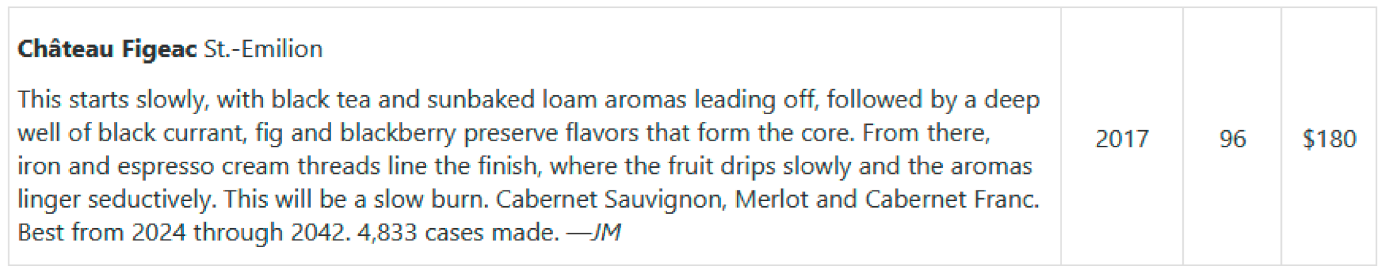
Wine Spectator is a wine magazine company that provides wine reviews periodically by a group of wine region specific reviewers, “Wine spectator started as a bi-weekly, California-based newsletter, but has since become the world’s leading authority on wine.” [48] The magazine publishes 15 issues a year, and there are between 400 to 1000 wine reviews per issue. In previous Wineinformatics research [14], more than 100,000 wine reviews were gathered and analyzed across all wine regions in the world. This dataset was used to test wine reviewers’ accuracy in predicting a wine’s credit score. Wine Spectator reviewers received more than 87% accuracy when evaluated with the SVM method while predicting whether a wine received a credit score higher than 90/100 points [7]. The satisfactory results demonstrate that Wine Spectator provides consistent wine reviews. Moreover, in the same study, James Molesworth who reviews all Bordeaux wines was ranked number three among all reviewers. Therefore, the Bordeaux wine reviews retrieved from Wine Spectator are suitable for this research. Figure 1 provides an example of Wine Spectator’s review describing the 2017 Chateau Figeac (96 points in 100 points scale and cost $180 per bottle) from St. Emilion, Bordeaux which won #57 in Wine Spectator’s 2020 Top100 wines [49].
2.2. Bordeaux Dataset
Bordeaux (“Bore-doe”) refers to a wine from Bordeaux, France. A massive portion of the wines produced by this region are red wines (over 90%) with Merlot or Cabernet Sauvignon. Bordeaux is the largest AOC vineyard of France and has 54 appellations [50]. As this region provides such a large portion of red wines, a large amount of the reviews utilized in this project and a considerable amount of the attribute distribution will be in favor of red wines. However, Bordeaux does produce other varieties of wines, and even within the red wines that are produced in this region, there exists differences based off the terroir, that being the environment in which a wine is produced, and the vintage of the wines as well.
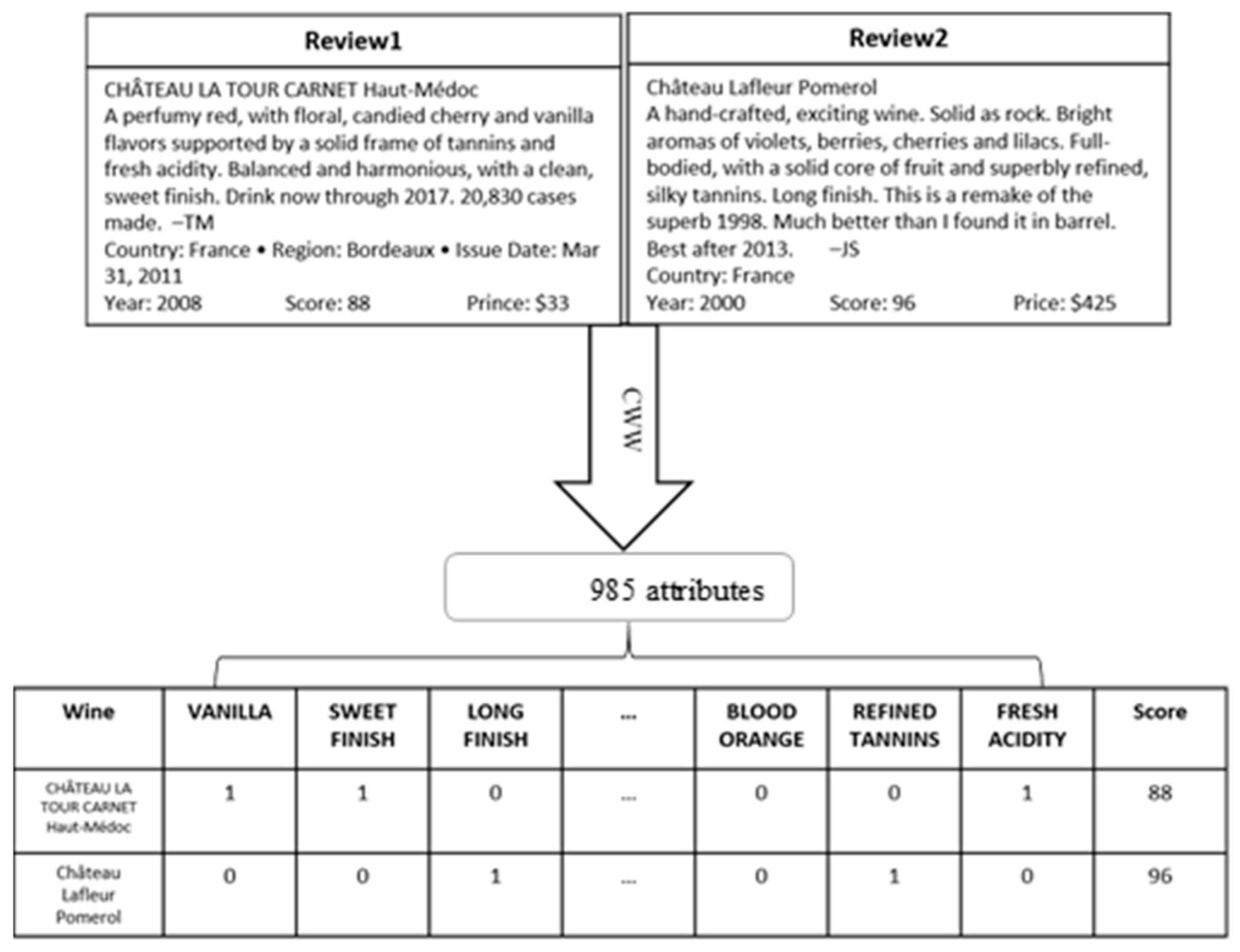
In our previous research [34], we explored all 21st century Bordeaux wines by creating a publicly available dataset with 14,349 Bordeaux wines [35] that covers all available Bordeaux wine reviews from year 2000~2016 from Wine Spectator. Since all of the reviews are in human language format as shown in Figure 1, the reviews ar e processed by the Computational Wine Wheel [21,22] which works as a dictionary using one-hot encoding to convert words into vectors. For example, in a wine review, there are some words that contain fruits such as apple, blueberry, plum, etc. If the word matches the attribute in the computation wine wheel, it will be 1; otherwise, it will be 0. Binary data represent a method of data classification where the data exists in either one state or the other. It is numerically represented by a combination of zeros and ones. The Computational Wine Wheel is also equipped with a generalization function to map similar words into the same coding. For example, fresh apple, apple, and ripe apple are generalized into “Apple” since they represent the same flavor; however, green apple belongs to “Green Apple” since the flavor of green apple is different from apple. The score of the wine is also attached to the data as the last attribute, also known as the label. This pre-processing step is crucial for computers to “understand” the wine reviews. Figure 2 provides a visual example of the process.
While this information can be useful to the consumer and profitable to vendors, in its current state, the dataset is difficult to interpret for results. As stated above, it is not practical to expect any vendor to carry all the wines in the dataset, and it would be a sizable task to sift through this information and extract any specific wine or feature to focus on. The initial idea was to perform an unsupervised approach to find common attributes of the listed wines and group them together based on these similarities. A further issue became apparent as the data was analyzed. The data provides binary attributes for all possible values that can be provided by the wine wheel. Among these values are more general terms such as “finish”, “fruit”, and “great”. These values represent common attributes appearing at a higher rate than other attributes, but these values are not exactly interesting for finding similarities within groups of clusters. Before moving forward with further grouping of the wines, such values need to be removed to allow for better results when looking to group the wines and find the most common attributes between them. To accomplish this, attributes were removed from the overall list of attributes. The determined threshold was that any wine attribute that appears in over 20% of the listed wines (around 2870 wines) or more was removed. This resulted in the removal of six attributes from the dataset.
3. Methods
3.1. K-Means Clustering
Unsupervised machine learning algorithms infer patterns from a dataset without reference to known or labeled outcomes [2]. What separates this from the supervised machine learning algorithms is the fact that when this type of learning is performed there is no knowledge as to what we are going to observe in the results. Among the unsupervised learning algorithms are various methods of clustering, which is the grouping of a particular set of objects based on their characteristics, aggregating them according to their similarities. While there are different methods of clustering that can be performed, this project turned to the use of K-Means clustering [51] as it is a familiar method that is well known and tested.
K-Means clustering might be the simplest and the most popular unsupervised machine learning algorithm. In K-Means clustering, the K value refers to the number of centroids (clusters). When a number K is defined, we then calculate the distance from a point to each centroid such that for every point we check the distance between this point and all centroids. The centroid with the minimum distance in relation to the point will define which cluster a point belongs to. When using K-Means clustering, a major factor in the calculation is the distance calculation. For most applications, the use of Euclidean distance or Manhattan distance formulas is utilized, but these are not accurate for the use of distance calculations of binary data. To account for this problem, the Jaccard distance formula shown in equation 1 is used in place of the standard Euclidean distance formula.
where P = Number of variables positive for both objects, Q = Number of variables positive in Q, but not R, R = Number of variables positive in R, but not Q. The short Jaccard’s distance, the similar two objects are. A value of 0 in the distance is completely similar and a value of 1 is completely dissimilar.
Using Table 1 to demonstrate this calculation for the distance between A and B, that is dAB, we find the values for the distance calculation defined above. The three variables that are specifically needed are p, q, and r. The calculation for p would correlate to Item1 as both A and B are positive for the case in Item1, so P = 1. The calculation for Q correlates to Item3 and Item5 where the values for A are positive (1), and the values for B are negative (0), so Q = 2. The calculation for r correlates to Item2 where A is negative (0), and B is positive (1). With these two values, the calculation for dAB would be (2 + 1)/(1 + 2 + 1). This results in a Jaccard distance from A to B of 0.75.
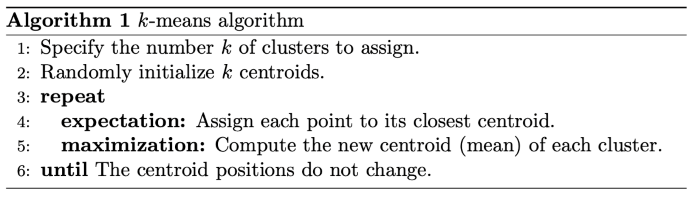
The original K-means clustering can be described as shown in Figure 3 [7]. With a user-defined K as the number of clusters, the program will randomly choose the initial centroids location. After that, a repeat process will occur to assign existing points to the closest centroids by calculating the distances to all centroids based on the given distance calculation formula. After all points are assigned, recalculate the centroid location and repeat the process until no changes on the centroid location or some pre-defined convergence criteria.
3.2. Filtering Process
Before clustering the wine information, this research attempts to apply some filtering processes to extract more precise and meaningful information since both the number of wines and attributes are large. Two separate methods were used to filter this data before performing the K-Means clustering algorithm.
3.2.1. Filtering Method 1: Attributes Filtration
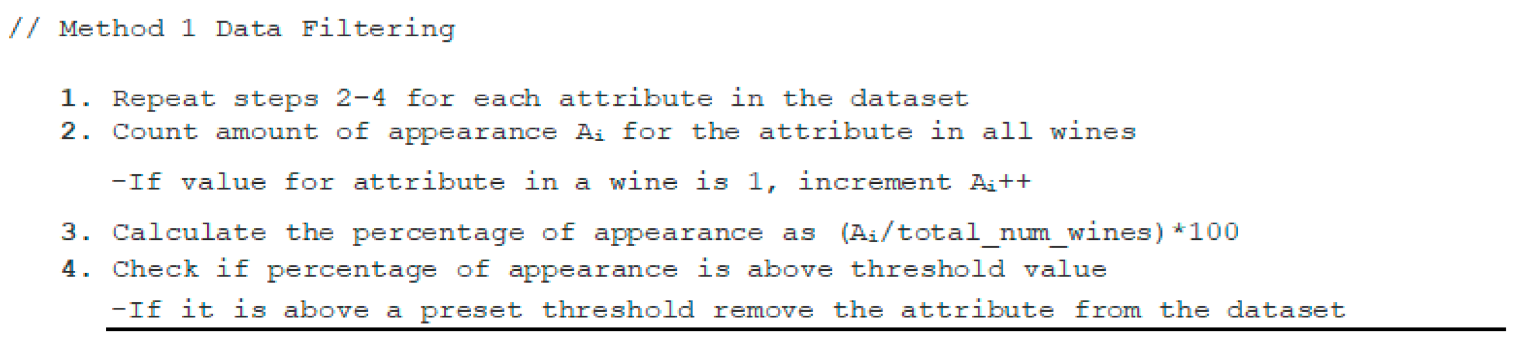
Method one filtered the characteristics of the wine based on overall appearance within the dataset. This ensured that overly common attributes (“FINISH”, “TANNINGS”, etc.) were removed from the calculation to avoid wines being clustered based on these attributes. The selection for which attributes to remove was based on a percentage calculation based on the overall number of wines relating to how many of these wines has this attribute present. Multiple tests were performed on 10% increments, and the best results were observed when attributes appearing in 20% of the wines or more are removed. The pseudo code for filtering method 1 is given in Figure 4.
3.2.2. Filtering Method 2: Wine Grade Filtration + Attributes Filtration
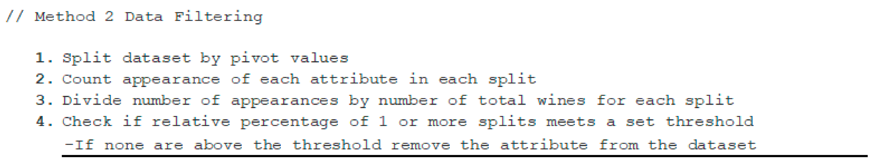
The second method involved choosing an attribute as a pivot and building distribution ratios for all wine wheel attributes based on that pivot. It makes the most sense for the pivot attribute to be one that was not generated by Computational Wine Wheel. Instead, it should be chosen from the other available attributes such as Price, Score, time of harvest, etc. For this project, Score was selected to be the pivot point. Starting from the selection of 432 wines with a score of 95 and greater, they were then split into three sub-groups. These consisted of wines with scores of 95, wines with scores of 96–97, and wines with scores of 98–100. This split allowed for a relatively even distribution, leading to sets of 165, 202, and 70 wines, respectively. A total was then taken for each wine wheel attribute. These totals represented the total number of wines within each sub-group that contained the given attribute. The totals were weighted to account for the variation of the sub-group size used to generate three ratios showing each sub-group’s representation of each wine wheel attribute. For the purposes of this method, attributes whose distribution was too even were tossed out for clustering. Three subsets of data were generated using distribution thresholds. These thresholds were 50%, 55%, and 60%, meaning if one sub-group of wines carried a weighted representation of 50% or more for a given wine wheel attribute, it was selected to remain in the 50% subset. The pseudo code for filtering method 2 is given in Figure 5.
3.3. Proposed K-Means Clustering with Optimal K Search and Filtration Process
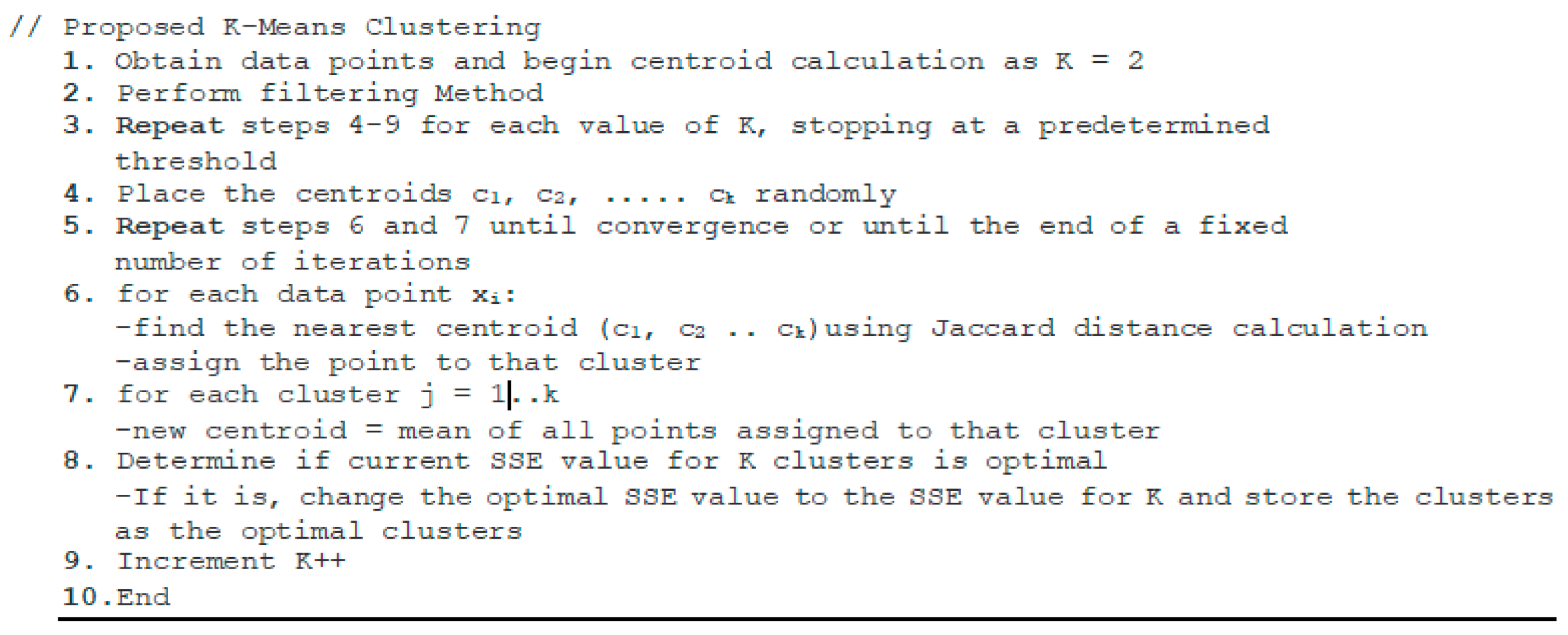
In this research, we proposed a modified K-means clustering algorithm to cluster the Bordeaux wine dataset based on the original K-means clustering, Jaccard’s Distance and filtering methods. The following method shown in Figure 6 is the clustering algorithm that is performed on the data after filtering:
The first step of the clustering is read in the data and set the K value starts with 2, representing 2 clusters. After that, one of the filtering methods is applied to remove unwanted information. Steps 3~7 are the original K-means clustering algorithm where the initial centroids are calculated using the random selection method. This method chooses random points from the dataset and sets those as the starting centroids that all points are compared to. After all points are clustered using the initial centroids, the new centroids are calculated using a threshold value based on the number of times each feature is present in the wines in the cluster. A base value of 30% is used as the lowest threshold value allowed for a feature to become part of the new centroid, meaning that if the attribute in question is present (value of 1) 30% of the time or more, then the value for that feature in the new centroid of that cluster is a 1, otherwise it is a 0. This allows for unique features to still be evaluated as part of the selection, since some features can appear in less than one percent of the wines.
Step 8 is used to evaluate the quality of the cluster. When performing K-Means clustering, a method must be used to calculate the validity of the clusters formed. This is useful for knowing if the clustering algorithm is performing correctly, as well as showing which value K results in the best clusters. The method utilized in this project relies on the use of the SSE (Sum of the Squares due to Error) values
The formula calculates the variation within the clusters, where n is the number of observations and Xi is the value of the ith observation. A cluster that consists of identical items would result in a SSE value of zero. When utilized in cluster evaluation, we can take the minimum SSE value and use it as a measure of when the wines in each cluster are most similar to each other.
After steps 3~8 are executed, Step 9 will increment the K value by one and repeat the whole process with the new K value. Therefore, after the first try of the K = 2, step 9 will increase K to 3 and repeat the whole K-means clustering and evaluate the result. Once K = 3 is done, K will change to 4 and repeat the whole process and so on.
4. Results
4.1. Clustering with Attributes Filtration
For the first part of the result, the data is first filtered by the approach described in Section 3.2.1 and then clustered utilizing the full 14,349 wines in the dataset. One hundred runs are performed on each K value possible, with a maximum number of one hundred iterations allowed for the program to successfully separate the wines into their best clusters. This is done while determining the SSE values for each run and keeping track of which run produced the best SSE value and what that SSE value was. Once the optimum K value is obtained, the clustering algorithm was performed multiple times using only the optimum value for K to determine if this value produced consistently useful results.
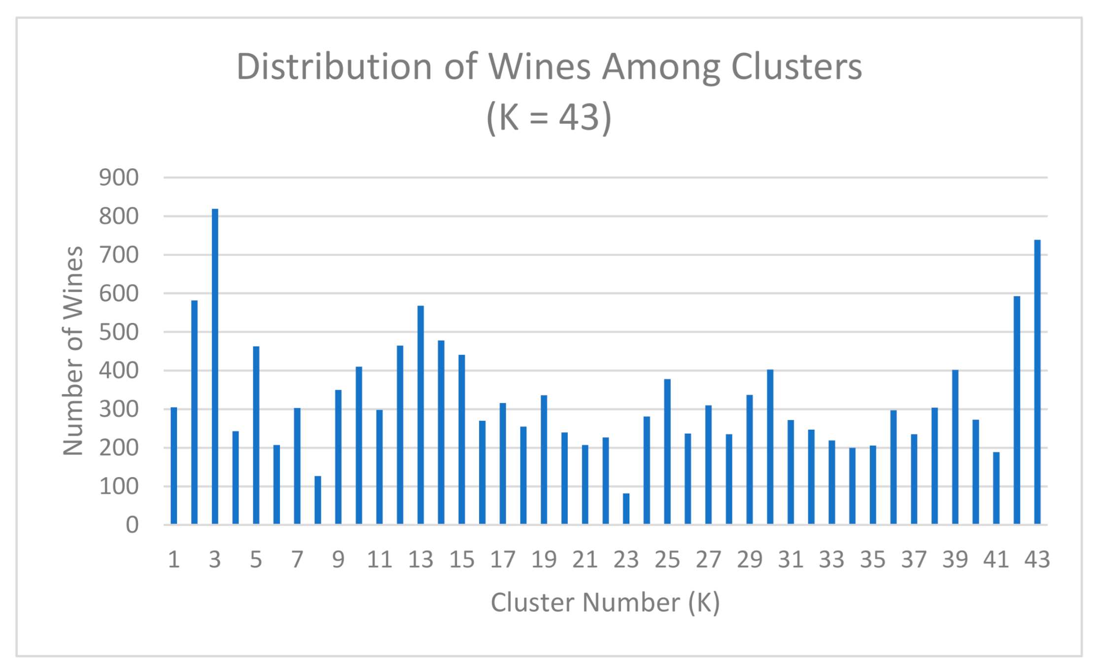
Utilizing this method, the optimum number of clusters K was determined to be 43. Based on this information, the clusters were formed after 50 runs of K-means clustering to determine the best formed clusters utilizing 43 as the K value. These clusters were then used to extract the following information for each cluster: Number of Points in Cluster, Average Year, Year Standard Deviation, Average Score, Score Standard Deviation, Most Common Attribute, Second Most Common Attribute, and Third Most Common Attribute. From these clusters, we also determined the wine from each cluster that best represents the cluster as a whole as shown in Table 2. This wine is determined as the wine with attributes that are most similar to the final centroid value for each cluster. A percentage value was utilized to determine which wine was the most similar to each centroid, and the percentage values that resulted ranged from 97.38–99.51% in similarity.
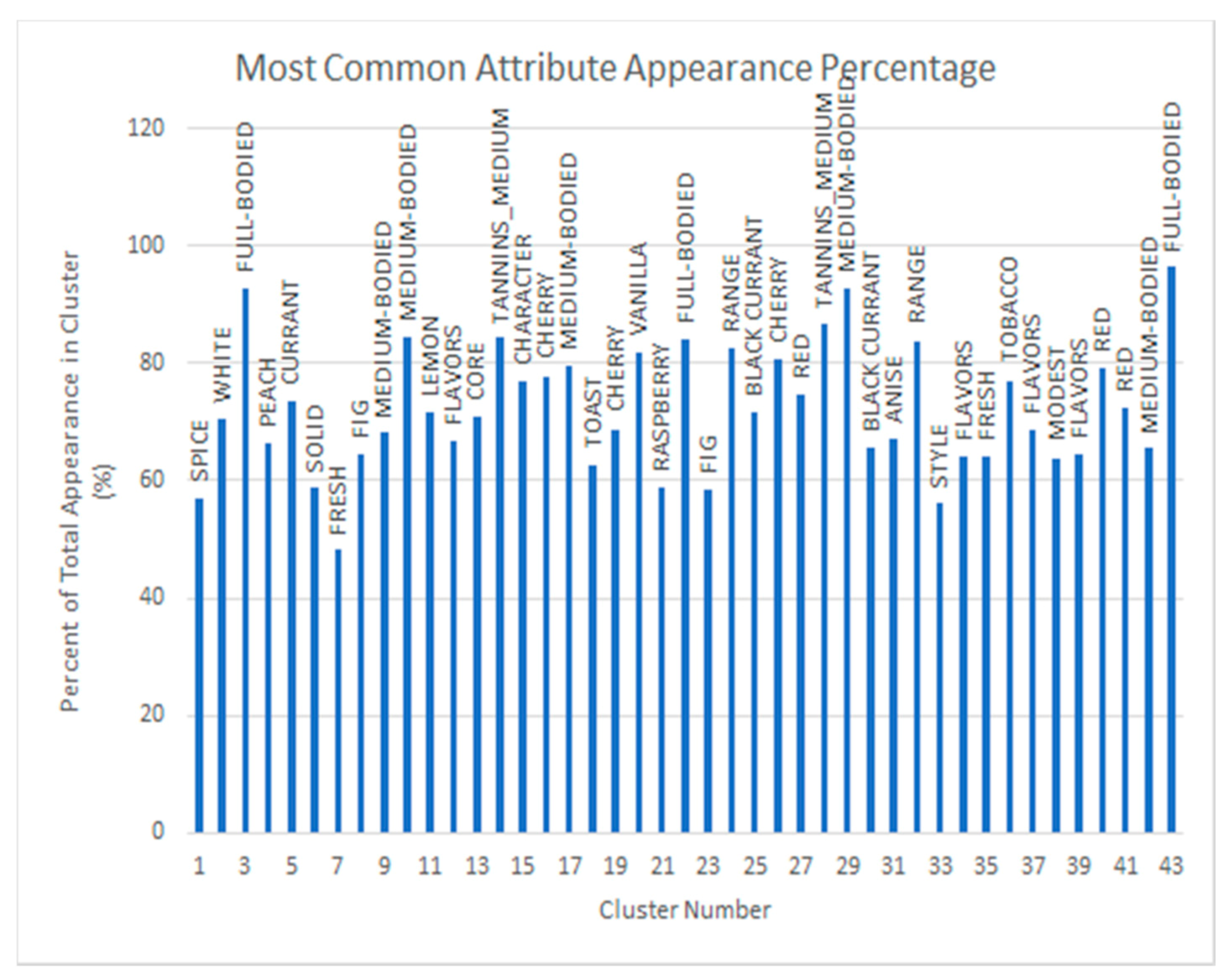
Figure 7 shows the distribution of wines within each cluster when K = 43. Based on the shown information, we know that the majority of the clusters contain a range of 200 or more wines. However, the diversity of the amounts within each cluster show that the wines have been grouped successfully based on their attributes, as further illustrated in Figure 8 and Figure 9 where the most common and second most common attributes are shown per each cluster. This gives more information into what characteristics the wines listed in Table 2 contain that shows them as the best representation of their clusters. For example, if we look at cluster 10, we see that Romulus Pomeroi from the year 2008 is the best wine to represent this cluster. It has a score of 90, making it an outstanding wine by the scoring scale. We also see that this wine can most likely be described as “medium-bodied” and that the “character” of this wine stands out well.
Figure 10 shows the average wine score in each cluster with standard deviation. Since the wine score was not included in the clustering process as an attribute, we can use Figure 10 to understand more about each cluster. If we look into cluster 38, we can see that it has the lowest average score for the collection of wines within. When we look further into the common attributes of the cluster, we can determine that a combination of “modest” and “herbs” reflections result in a less desirable wine than any other noted combination. This would also imply that Château Pipeau St.-Emilion 2007, which likely contains the combination of features, would probably be less favorable on this list for vendor sales.
Figure 11, Figure 12, Figure 13 and Figure 14 and Table 3 illustrate the possible use of the algorithm when a different number of clusters are desired. This demonstrates that if researchers wanted a smaller list of representative wines to select from, then, the proposed method can change the number of clusters to represent that. This is also true for desiring a larger number of wines to select from as well. While the optimal K value was determined to be 43, that does not restrict this program from creating larger or smaller clusters. The major differences when altering the cluster sizes are the number of wines placed into a cluster, the average calculations derived from the clusters, and the number of common attributes that are possible.
4.2. Clustering with Wine Grade Filtration + Attributes Filtration
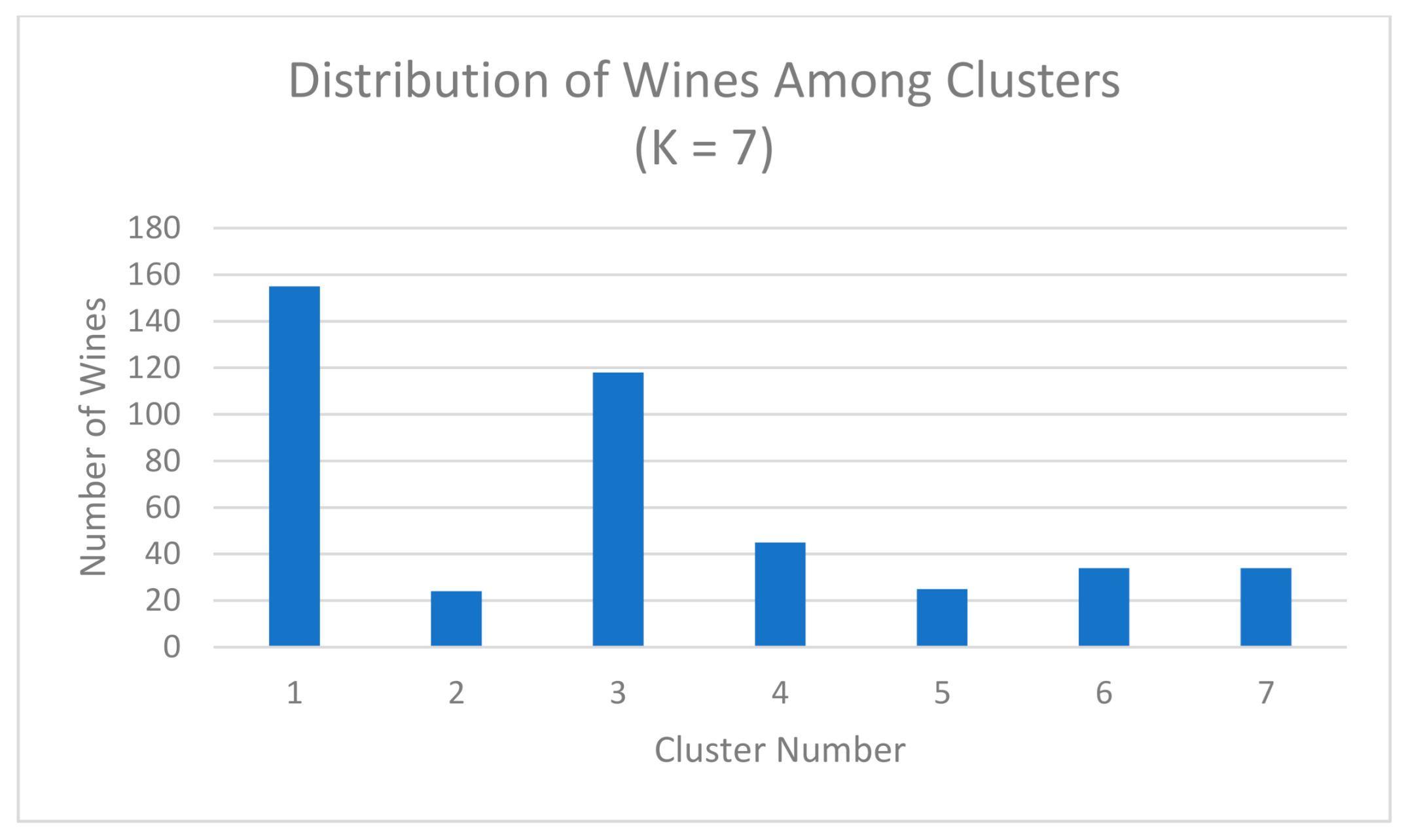
For the second part of the result, the wines and attributes are filtered by the method described in Section 3.2.2. While the wine grade threshold was set to 95 points, 435 wines remained after the filter process. The overall goal of this method is to cluster high end Bordeaux wines so that vendors and wine lovers alike might use the resulting clusters to develop a selection of wines that encompasses the wide range of characteristics that can describe Bordeaux. The same approach was used as in Section 4.1 for determining the optimal K value. 7 clusters seem the best choice for the smaller but elite dataset. The clustering results are relatively evenly distributed clusters compared to unfiltered attempts, as well as highly unique and interesting Highest Common Attribute. It was determined that the 60% and 65% subsets were throwing out interesting attributes like BLACK-TEA and BLOOD ORANGE so it was decided that the focus would continue on the 50% subset. When applying this method to different datasets, these comparisons would still prove useful but require human decision making as to which thresholds are best. The number of wines contained in each cluster contained between 24 and 155 wines is illustrated in Figure 15.
The most common and second most common attributes and their percentage of appearance are listed in Table 4 and Table 5, respectively. The low percentage of appearance of DEEP within Cluster 1 suggests that the wines in this cluster may not be as well grouped as the wines in the others. If a user were to look into the specific wines of each cluster in order to make a selection, this cluster may need to be either left out or simply used to fill out any remaining space in their offerings. The best representation for each cluster is given in Table 6. For the purposes of this dataset, average score and the standard deviation did not provide any meaningful insight, which was not surprising given that so few scores were included.
The highest common attributes actually hinted at another potential use of this process. Not only are the wines now clustered into unique subcategories within high end Bordeaux, but potential names for these categories are given by these highest common attributes. A wine vendor could use the attribute names themselves as sub-categories for Bordeaux that they offer their patrons. For example, if they chose the wine Liber Pater Graves from cluster 1, they could advertise/offer it to their customers under the moniker Deep, even if that specific wine did not end up with a reviewer using that specific word. This would in turn simplify and clarify the choice of what to purchase for the customers themselves.
Each of the two methods described in this project have shown to be very promising in the objective of composing an all-encompassing list of wines that represents the full range of flavors and textural characteristics that can be used to describe Bordeaux wines.
5. Conclusions
Wineinformatics is a new data science research area that focuses on large amounts of wine-related data. In this research, unsupervised analysis was applied on 14,349 wines to select representative 21st century Bordeaux wines. A systematic process that incorporates K-means clustering with optimal K search and filtration process was proposed and carried out in this work. Detail clustering results constructed from two different filtering methods, where the first method looks at the overall presence of each attribute and the second method focuses on attribute distribution based on a user defined pivot, were provided in the result section. Both have shown promise for generating unique clusters of wines, and both should be considered for any real-world use cases.
The intended use of these methods is for wine vendors to make a selection given the limited number of wines they can realistically offer. These wines will hopefully represent a broad range of flavor profiles within a given dataset and therefore please the widest market. Wine connoisseurs can also try the list of representative wines of the clusters to understand the variety of the wine region with as few wines as possible. Another use of the cluster could be the recommendation system. A cluster of wine represents wines with similarity; a consumer who enjoyed a representative wine from the cluster can be recommended other wines in the cluster with higher (or lower) price.
The dataset presented in the paper focuses on 21st century Bordeaux with vintage covers from year 2000~2016. Many possible researches can adopt the same process to analyze and find representative wines in a different wine making region/country; vintage(s); or pivot points such as price, weather, terroir, etc. This finding has strong impacts on all Wineinformatics research in many different topics about wine, which has the potential to provide useful information to wine makers, consumers, and distributors.
Author Contributions
J.M., A.R. program, designed the experiment and original writing. And B.C. literature review, conceived research ideas, original writing, revise and refine the manuscript. All authors have read and agree to the published version of the manuscript.
Funding
This research received no external funding.
Institutional Review Board Statement
Not applicable.
Informed Consent Statement
Not applicable.
Data Availability Statement
Not applicable.
Conflicts of Interest
The authors declare no conflict of interest.
References
- Caruana, R.; Niculescu-Mizil, A. An Empirical Comparison of Supervised Learning Algorithms. In Proceedings of the 23rd International Conference on Machine Learning, ICML ’06, New York, NY, USA, 25–29 June 2006; pp. 161–168. [Google Scholar]
- Hastie, T.; Tibshirani, R.; Friedman, J. Unsupervised Learning; Springer: New York, NY, USA, 2009; pp. 485–585. [Google Scholar]
- Zhu, X.; Goldberg, A.B. Introduction to semi-supervised learning. In Synthesis Lectures on Artificial Intelligence and Machine Learning; Morgan and Claypool Publishers: San Rafael, CA, USA, 2009; Volume 3, pp. 1–130. [Google Scholar]
- Levine, S. Reinforcement learning and control as probabilistic inference: Tutorial and review. arXiv 2018, arXiv:1805.00909. Available online: https://arxiv.org/abs/1805.00909 (accessed on 1 January 2021).
- Karlsson, P. World Wine Production Reaches Record Level in 2018, Consumption is Stable. Available online: https://www.bkwine.com/features/more/world-wine-production-reaches-record-level-2018-consumption-stable/ (accessed on 14 April 2019).
- Forbes. Global Wine Production 2019 is Returning to ‘Normal’, Says Pau Roca of the OIV. Available online: https://www.forbes.com/sites/karlsson/2019/11/03/global-wine-production-2019-of-263-mhl-is-a-return-to-normal-says-pau-roca-of-the-oiv/?sh=7a97ff5c745b (accessed on 21 November 2020).
- Han, J.; Pei, J.; Kamber, M. Data Mining: Concepts and Techniques; Elsevier: Amsterdam, The Netherlands, 2011. [Google Scholar]
- Di Vita, G.; Chinnici, G.; D’Amico, M. Clustering attitudes and behaviours of Italian wine consumers. Calitatea 2014, 15, 54. [Google Scholar]
- Hall, D. Exploring wine knowledge, aesthetics and ephemerality: Clustering consumers. Int. J. Wine Bus. Res. 2016, 28, 134–153. [Google Scholar] [CrossRef]
- Vázquez-Fresno, R.; Llorach, R.; Perera, A.; Mandal, R.; Feliz, M.; Tinahones, F.J.; Wishart, D.S.; Andres-Lacueva, C. Clinical phenotype clustering in cardiovascular risk patients for the identification of responsive metabotypes after red wine polyphenol intake. J. Nutr. Biochem. 2016, 28, 114–120. [Google Scholar] [CrossRef] [PubMed] [Green Version]
- Esteban-Fernández, A.; Ibañez, C.; Simó, C.; Bartolomé, B.; Arribas, V.M. Metabolome-based clustering after moderate wine consumption. OENO One 2020, 54, 455–467. [Google Scholar] [CrossRef]
- Gelbard, R.; Goldman, O.; Spiegler, I. Investigating diversity of clustering methods: An empirical comparison. Data Knowl. Eng. 2007, 63, 155–166. [Google Scholar] [CrossRef]
- Venkataramana, B.; Padmasree, L.; Rao, M.S.; Rekha, D.; Ganesan, G. A Study of Fuzzy and Non-fuzzy clustering algorithms on Wine Data. Commun. Adv. Comput. Sci. Appl. 2017, 2017, 129–137. [Google Scholar] [CrossRef] [Green Version]
- Chen, B.; Velchev, V.; Palmer, J.; Atkison, T. Wineinformatics: A Quantitative Analysis of Wine Reviewers. Fermentation 2018, 4, 82. [Google Scholar] [CrossRef] [Green Version]
- Palmer, J.; Chen, B. Wineinformatics: Regression on the Grade and Price of Wines through Their Sensory Attributes. Fermentation 2018, 4, 84. [Google Scholar] [CrossRef] [Green Version]
- Cortez, P.; Cerdeira, A.; Almeida, F.; Matos, T.; Reis, J. Modeling wine preferences by data mining from physicochemical properties. Decis. Support Syst. 2009, 47, 547–553. [Google Scholar] [CrossRef] [Green Version]
- Ting, S.L.; Tse, Y.K.; Ho, G.T.S.; Chung, S.H.; Pang, G. Mining logistics data to assure the quality in a sustainable food supply chain: A case in the red wine industry. Int. J. Product. Econom. 2014, 152, 200–209. [Google Scholar] [CrossRef]
- Ishibuchi, H.; Nakashima, T.; Nii, M. Classification and Modeling with Linguistic Information Granules: Advanced Approaches to Linguistic Data Mining; Springer: Berlin/Heidelberg, Germany, 2005. [Google Scholar]
- Urtubia, A.; Pérez-Correa, J.R.; Soto, A.; Pszczólkowski, P.; Pérez-Correa, J.R. Using data mining techniques to predict industrial wine problem fermentations. Food Control 2007, 18, 1512–1517. [Google Scholar] [CrossRef]
- Edelmann, A.; Diewok, J.; Schuster, K.C.; Lendl, B. Rapid method for the discrimination of red wine cultivars based on mid-infrared spectroscopy of phenolic wine extracts. J. Agric. Food Chem. 2001, 49, 1139–1145. [Google Scholar] [CrossRef]
- Chen, B.; Rhodes, C.; Crawford, A.; Hambuchen, L. Wineinformatics: Applying Data Mining on Wine Sensory Reviews Processed by the Computational Wine Wheel. In Proceedings of the 2014 IEEE International Conference on Data Mining Workshop, Shenzhen, China, 14 December 2014; pp. 142–149. [Google Scholar]
- Chen, B.; Rhodes, C.; Yu, A.; Velchev, V. The Computational Wine Wheel 2.0 and the TriMax Triclustering in Wineinformatics. In Advances in Data Mining. Applications and Theoretical Aspects, Proceedings of the Industrial Conference on Data Mining, New York, NY, USA, 18–20 July 2016; Springer: Cham, Switzerland, 2016; pp. 223–238. [Google Scholar]
- Ducard, E. A Complete History of Bordeaux Wine, Tanglewood Wines Limited. 2018. Available online: https://tanglewoodwine.co.uk/blogs/news/complete-history-bordeaux-wine (accessed on 21 November 2020).
- Combris, P.; Lecocq, S.; Visser, M. Estimation of a hedonic price equation for Bordeaux wine: Does quality matter? Econ. J. 1997, 107, 389–402. [Google Scholar] [CrossRef]
- Cardebat, J.M.; Figuet, J. What explains Bordeaux wine prices? Appl. Econ. Lett. 2004, 11, 293–296. [Google Scholar] [CrossRef]
- Ashenfelter, O. Predicting the quality and prices of Bordeaux wine. Econ. J. 2008, 118, F174–F184. [Google Scholar] [CrossRef]
- Shanmuganathan, S.; Sallis, P.; Narayanan, A. Data Mining Techniques for Modelling Seasonal Climate Effects on Grapevine Yield and Wine Quality. In Proceedings of the 2010 2nd International Conference on Computational Intelligence, Communication Systems and Networks, Liverpool, UK, 28–30 July 2010; pp. 84–89. [Google Scholar]
- Noy, F.N.; Sintek, M.; Decker, S.; Crubézy, M.; Fergerson, R.W.; Musen, M.A. Creating semantic web contents with protege-2000. IEEE Intell. Syst. 2001, 16, 60–71. [Google Scholar] [CrossRef]
- Noy, F.N.; McGuinness, D.L. Ontology Development 101: A Guide to Creating Your First Ontology; Technical Report KSL-01-05 and Stanford Medical Informatics Technical Report SMI-2001-0880; Stanford Knowledge Systems Laboratory: Stanford, CA, USA, 2001. [Google Scholar]
- Quandt, R.E. A note on a test for the sum of rank sums. J. Wine Econ. 2007, 2, 98–102. [Google Scholar] [CrossRef] [Green Version]
- Ashton, R.H. Improving experts’ wine quality judgments: Two heads are better than one. J. Wine Econ. 2011, 6, 135–159. [Google Scholar] [CrossRef]
- Ashton, R.H. Reliability and consensus of experienced wine judges: Expertise within and between? J. Wine Econ. 2012, 7, 70–87. [Google Scholar] [CrossRef]
- Bodington, J.C. Evaluating wine-tasting results and randomness with a mixture of rank preference models. J. Wine Econ. 2015, 10, 31–46. [Google Scholar] [CrossRef]
- Dong, Z.; Guo, X.; Rajana, S.; Chen, B. Understanding 21st Century Bordeaux Wines from Wine Reviews Using Naïve Bayes Classifier. Beverages 2020, 6, 5. [Google Scholar] [CrossRef] [Green Version]
- Chen, B. Wineinformatics: 21st Century Bordeaux Wines Dataset. IEEE Dataport. 2020. Available online: https://ieee-dataport.org/open-access/wineinformatics-21st-century-bordeaux-wines-dataset (accessed on 1 January 2021).
- Chen, B.; Velchev, V.; Nicholson, B.; Garrison, J.; Iwamura, M.; Battisto, R. Wineinformatics: Uncork Napa’s Cabernet Sauvignon by Association Rule Based Classification. In Proceedings of the 2015 IEEE 14th International Conference on Machine Learning and Applications, Miami, FL, USA, 9–11 December 2015; pp. 565–569. [Google Scholar]
- Rhodes, C.T. Wine Informatics: Clustering and Analysis of Professional Wine Reviews. Master’s Thesis, University of Central Arkansas, Conway, AR, USA, May 2015. [Google Scholar]
- Chen, B.; Buck, K.H.; Lawrence, C.; Moore, C.; Yeatts, J.; Atkison, T. Granular Computing in Wineinformatics. In Proceedings of the 2017 13th International Conference on Natural Computation, Fuzzy Systems and Knowledge Discovery, Guilin, China, 29–31 July 2017; pp. 1228–1232. [Google Scholar]
- Bird, S.; Klein, E.; Loper, E. Natural Language Processing with Python: Analyzing Text with the Natural Language Toolkit; O’Reilly Media, Inc.: Sebastopol, CA, USA, 2009. [Google Scholar]
- Wine School of Philadelphia. Wine Reviews: The Essential Guide Featured. 20 November 2019. Available online: www.vinology.com/wine-review-guide/ (accessed on 21 November 2020).
- Wine Searcher. What Are Wine Scores? Available online: www.wine-searcher.com/wine-scores (accessed on 21 November 2020).
- Cardebat, J.M.; Livat, F. Wine experts’ rating: A matter of taste? Int. J. Wine Bus. Res. 2016, 28, 43–58. [Google Scholar] [CrossRef] [Green Version]
- Cardebat, J.M.; Figuet, J.M.; Paroissien, E. Expert opinion and Bordeaux wine prices: An attempt to correct biases in subjective judgments. J. Wine Econ. 2014, 9, 282–303. [Google Scholar] [CrossRef]
- Cao, J.; Stokes, L. Evaluation of wine judge performance through three characteristics: Bias, discrimination, and variation. J. Wine Econ. 2010, 5, 132–142. [Google Scholar] [CrossRef] [Green Version]
- Cardebat, J.M.; Paroissien, E. Standardizing expert wine scores: An application for Bordeaux en primeur. J. Wine Econ. 2015, 10, 329–348. [Google Scholar] [CrossRef]
- Hodgson, R.T. An examination of judge reliability at a major US wine competition. J. Wine Econ. 2008, 3, 105–113. [Google Scholar] [CrossRef]
- Hopfer, H.; Heymann, H. Judging wine quality: Do we need experts, consumers or trained panelists? Food Qual. Prefer. 2014, 32, 221–233. [Google Scholar] [CrossRef]
- Sciaretta, G. Wine Spectator. About Us. 19 November 2020. Available online: www.winespectator.com/pages/about-us (accessed on 21 November 2020).
- Wine Spectator. Top 100 Wines. 2020. Available online: https://top100.winespectator.com/lists/ (accessed on 21 November 2020).
- Wine Folly. Bordeaux Wine 101: The Wines and the Region. 12 September 2019. Available online: www.Winefolly.com/deep-dive/a-primer-to-bordeaux-wine/ (accessed on 21 November 2020).
- Davidson, I. Understanding K-means non-hierarchical clustering. SUNY Albany Tech. Rep. 2002, 2, 2–14. [Google Scholar]
Figure 1.
An example of wine reviews on WineSpectator.com. Due to the changing monetary values of wines over time, price values are not considered in the filtering or clustering program.
Figure 1.
An example of wine reviews on WineSpectator.com. Due to the changing monetary values of wines over time, price values are not considered in the filtering or clustering program.

Figure 2.
The flowchart of converting reviews into machine language understandable through the computation wine wheel. All key word appearances for a review are initially recorded as a 0. When a key word is found within the review, it is recorded in the table as a 1.
Figure 2.
The flowchart of converting reviews into machine language understandable through the computation wine wheel. All key word appearances for a review are initially recorded as a 0. When a key word is found within the review, it is recorded in the table as a 1.

Figure 3.
Pseudo code for the K-means clustering algorithm. The initialization of the centroids is chosen from the already existing collection of data. The standard k-means algorithm utilizes Euclidean distance for assigning points their closest centroid, but this type of distance calculation does not work with regards to binary data (1 s and 0 s).

Figure 4.
Pseudo code for the filtering method 1: attribute filtration. We utilize Ai to account for an attribute (vanilla, cherry, finish, etc.), and we calculate the total appearance of this attribute in the entire dataset. When an attribute appears too often in the dataset, it can skew the results of the clustering algorithm.

Figure 5.
Pseudo code for the filtering method 2: Wine Grade Filtration + Attributes Filtration. The pivot value can be changed, but for our example we utilize a pivot based on scores.
Figure 5.
Pseudo code for the filtering method 2: Wine Grade Filtration + Attributes Filtration. The pivot value can be changed, but for our example we utilize a pivot based on scores.

Figure 6.
Pseudo code for the proposed K-means clustering with Optimal K search and Filtration Process. The major difference between this method and a standard k-means algorithm is which distance formula is used. The fixed number of iterations refers to the maximum number of times the centroids can be changed while the points are still shifting between clusters. The clusters typically reach the convergence threshold (are correctly grouped) before reaching the max number of iterations.0.

Figure 7.
Wines present in each cluster (K) with the optimum K value. For every cluster label (K), the total number of wines present in the cluster are shown. The groups shown reflect the distribution of similar wines across 43 different groups.
Figure 7.
Wines present in each cluster (K) with the optimum K value. For every cluster label (K), the total number of wines present in the cluster are shown. The groups shown reflect the distribution of similar wines across 43 different groups.

Figure 8.
Most common attributes per cluster at optimum cluster number (K = 43). The most common attribute of each cluster, or group, of wines is shown as a percentage of appearance in each cluster overall. Labels above the bars correlate to the percentage of appearance of that attribute in the cluster. These characteristics are typically the primary characteristics for grouping the wines.

Figure 9.
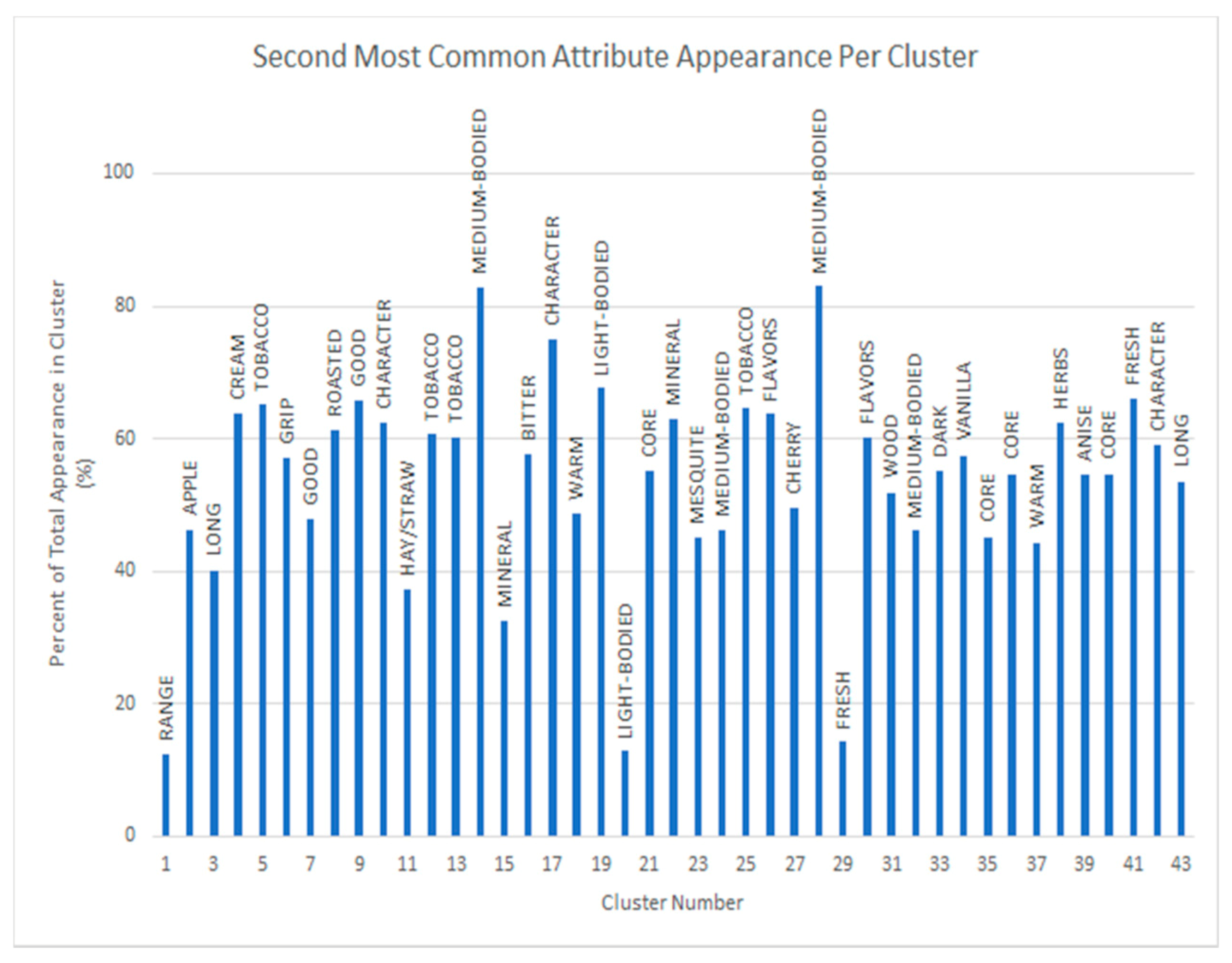
Second most common attributes per cluster at optimum cluster number (K = 43). The second most common attribute for each cluster, or group, of wines is shown as a percentage of appearance in each cluster overall. These values show a significant secondary characteristic grouping of each cluster, reflecting the necessity of utilizing all features of the wine reviews to group the wines accurately.
Figure 9.
Second most common attributes per cluster at optimum cluster number (K = 43). The second most common attribute for each cluster, or group, of wines is shown as a percentage of appearance in each cluster overall. These values show a significant secondary characteristic grouping of each cluster, reflecting the necessity of utilizing all features of the wine reviews to group the wines accurately.

Figure 10.
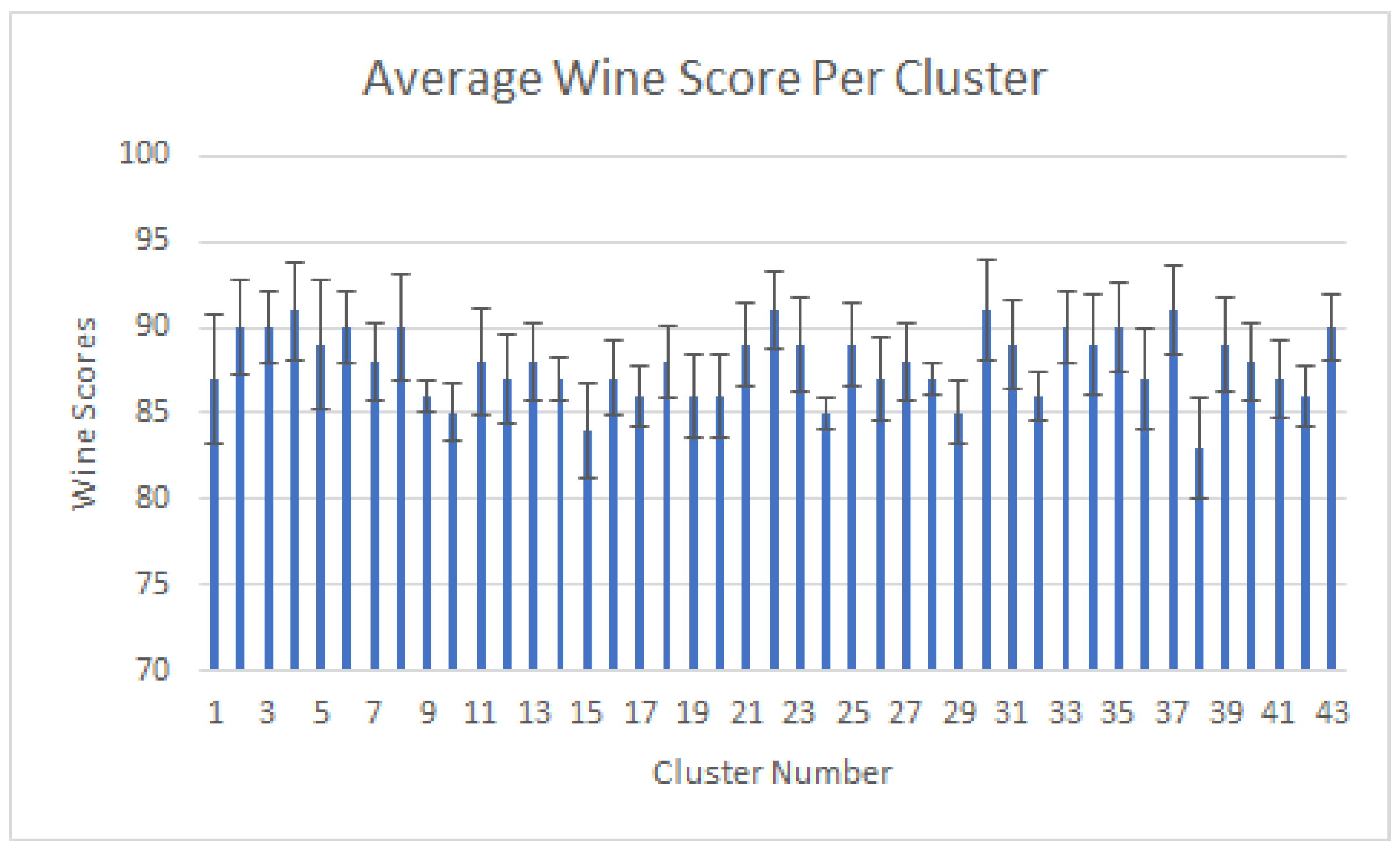
Average wine scores (±SD) per cluster with standard deviation. As the wine scores are not utilized when clustering the wines due to the focus on keywords within wine reviews, the wine scores given at the optimum cluster value (K = 43) are better utilized as a means of reflection as to which common attribute combination (Figure 8 and Figure 9) has better results.
Figure 10.
Average wine scores (±SD) per cluster with standard deviation. As the wine scores are not utilized when clustering the wines due to the focus on keywords within wine reviews, the wine scores given at the optimum cluster value (K = 43) are better utilized as a means of reflection as to which common attribute combination (Figure 8 and Figure 9) has better results.

Figure 11.
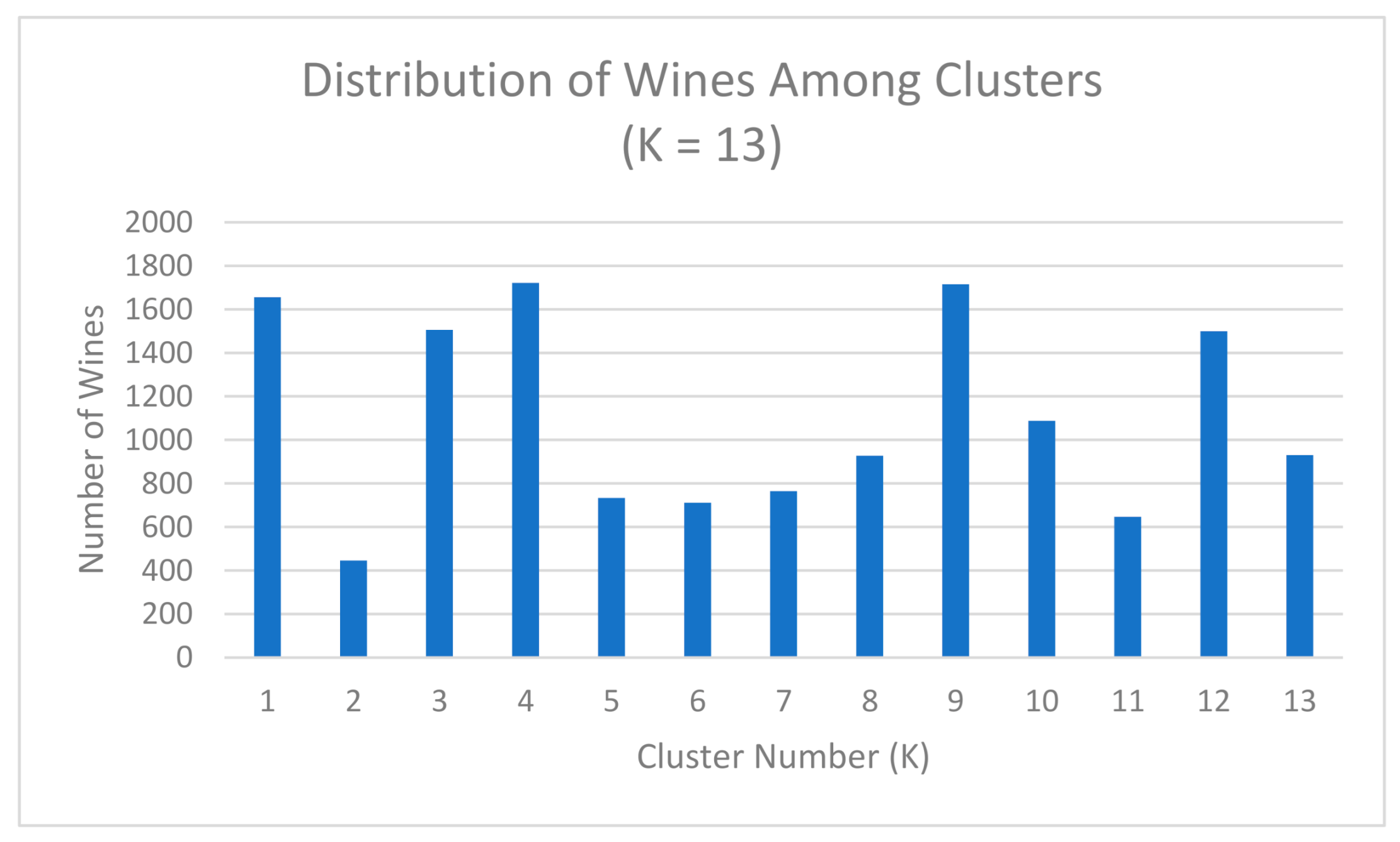
Number of wines per cluster with 13 Clusters. The main difference shown when changing the value of K is the change in population size of the clusters. While these clusters are still formed based on the similarities between the wines, the diversity of the wines within each cluster is greater than the diversity of the clusters when K = 43.
Figure 11.
Number of wines per cluster with 13 Clusters. The main difference shown when changing the value of K is the change in population size of the clusters. While these clusters are still formed based on the similarities between the wines, the diversity of the wines within each cluster is greater than the diversity of the clusters when K = 43.

Figure 12.
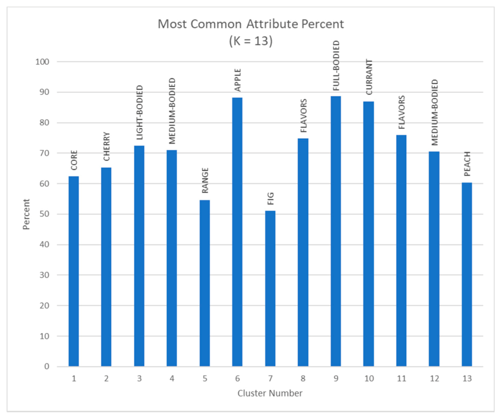
Most common attributes in each cluster when K = 13. The most common attribute percentages shown for each cluster label demonstrate that despite the changing K value, the program successfully groups the wines based on the most apparent attributes regardless of the increased diversity of the groups.
Figure 12.
Most common attributes in each cluster when K = 13. The most common attribute percentages shown for each cluster label demonstrate that despite the changing K value, the program successfully groups the wines based on the most apparent attributes regardless of the increased diversity of the groups.

Figure 13.
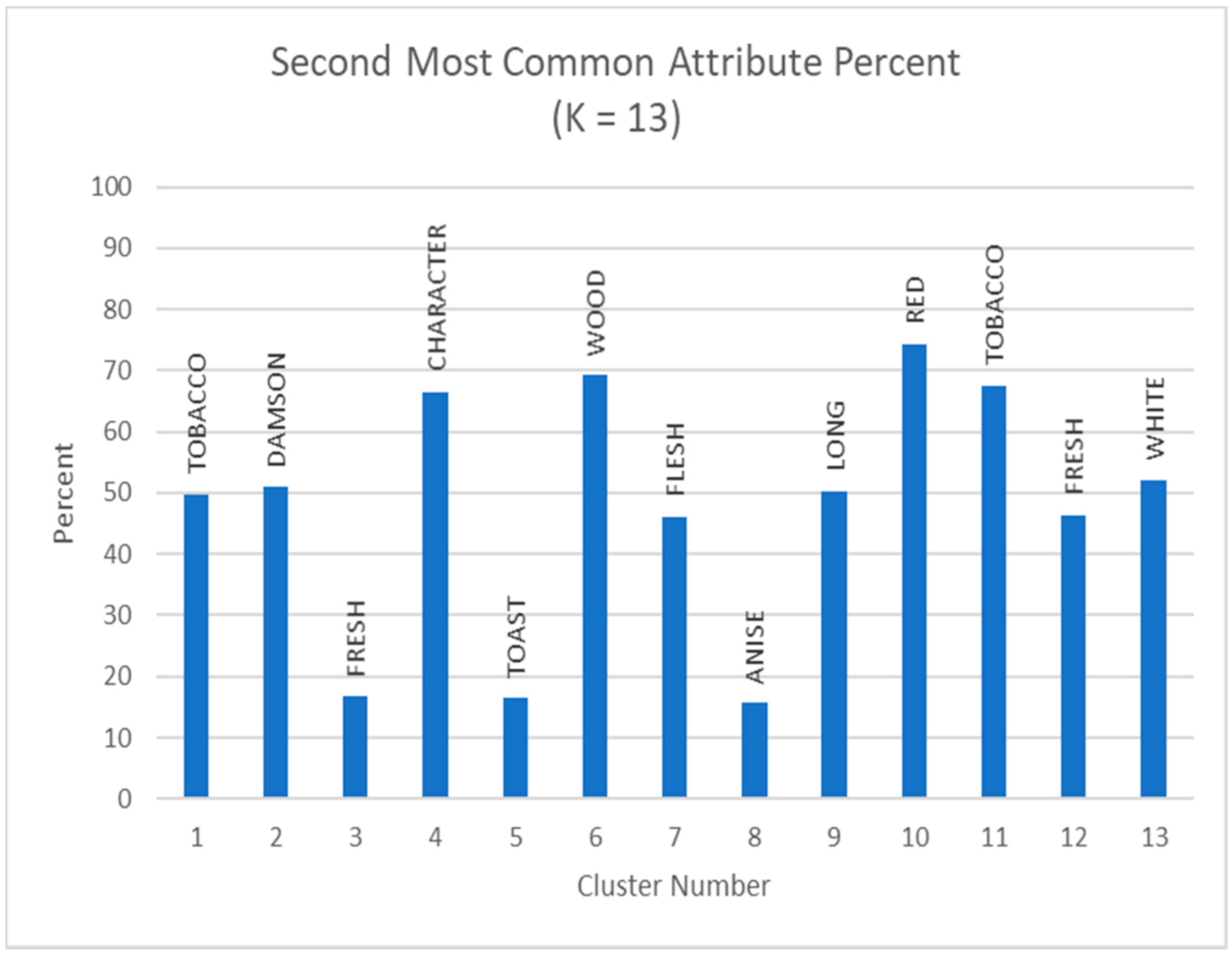
Second most common attributes in clusters when K = 13. The percentages shown do indicate that the increased populations of the clusters affect the common attributes of the clusters to an extent. A general decrease in percentage can be noted when utilizing a smaller K value.
Figure 13.
Second most common attributes in clusters when K = 13. The percentages shown do indicate that the increased populations of the clusters affect the common attributes of the clusters to an extent. A general decrease in percentage can be noted when utilizing a smaller K value.

Figure 14.
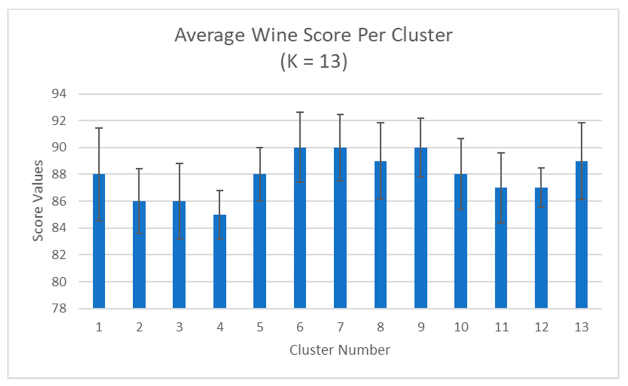
Average wine scores (±SD) per cluster when K = 13. The average wine scores of the clusters decreased overall. This can be attributed to the increased number of wines in each cluster as there exists a larger variation in scores for each cluster.
Figure 14.
Average wine scores (±SD) per cluster when K = 13. The average wine scores of the clusters decreased overall. This can be attributed to the increased number of wines in each cluster as there exists a larger variation in scores for each cluster.

Figure 15.
Number of wines per cluster with 7 clusters generated from the elite dataset. A smaller dataset and different method of feature removal accounts for the lower overall number of wines. Cluster 1 most likely represents a cluster consisting of wines that did not fit into any other clusters.
Figure 15.
Number of wines per cluster with 7 clusters generated from the elite dataset. A smaller dataset and different method of feature removal accounts for the lower overall number of wines. Cluster 1 most likely represents a cluster consisting of wines that did not fit into any other clusters.


Table 1.
Binary data example. For each label (A and B), the distance is calculated based on the comparison between the appearance of each item within that label. Jaccard distance is utilized for this type of data (binary).
Table 1.
Binary data example. For each label (A and B), the distance is calculated based on the comparison between the appearance of each item within that label. Jaccard distance is utilized for this type of data (binary).
| Wine | Item1 | Item2 | Item3 | Item4 | Item5 |
|---|---|---|---|---|---|
| A | 1 | 0 | 1 | 0 | 1 |
| B | 1 | 1 | 0 | 0 | 0 |
Table 2.
Best wine representations in each cluster at optimum cluster number (K = 43). The wines shown above, with their respective production years and scores, are the wines most similar to the centroid values of each cluster number. Each wine listed contains the closest similarities to all other wines within their respective group (cluster).
| Cluster Number | Wine Name | Wine Year | Wine Score |
|---|---|---|---|
| 0 | Château Suduiraut Sauternes | 2007 | 95 |
| 1 | Château Pape Clément Pessac-Léognan White | 2007 | 95 |
| 2 | Château L’Église Clinet Pomerol | 2009 | 98 |
| 3 | Château Haut-Brion Pessac-Léognan White | 2006 | 95 |
| 4 | Château Lyonnat Lussac-St.-Emilion Réserve de la Famille | 2005 | 87 |
| 5 | Château Latour Pauillac Les Forts de Latour | 2010 | 95 |
| 6 | Château Brown Pessac-Léognan White | 2006 | 90 |
| 7 | Château Langoa Barton St.-Julien | 2016 | 95 |
| 8 | Château Daugay St.-Emilion | 2009 | 90 |
| 9 | Romulus Pomerol | 2008 | 90 |
| 10 | Château Laville Haut-Brion Pessac-Léognan White | 2003 | 95 |
| 11 | Château Le Crock St.-Estephe | 2016 | 92 |
| 12 | Gracia St.-Emilion Les Angelots de Gracia | 2009 | 92 |
| 13 | Château Monregard La Croix Pomerol | 2009 | 90 |
| 14 | Château Pichon-Longueville Baron Pauillac | 2003 | 95 |
| 15 | Château Montrose St.-Estephe | 2016 | 96 |
| 16 | Château Lafleur Pomerol | 2007 | 92 |
| 17 | Château Carignan Premieres Cotes de Bordeaux | 2005 | 88 |
| 18 | Château Capet-Guillier St.-Emilion | 2016 | 90 |
| 19 | Château Laville Haut-Brion Pessac-Léognan White | 2006 | 93 |
| 20 | Château Bellevue-Mondotte St.-Emilion | 2005 | 97 |
| 21 | Château Haut-Brion Pessac-Léognan White | 2007 | 97 |
| 22 | Château Pontet-Canet Pauillac | 2003 | 93 |
| 23 | Château Lamothe Sauternes | 2009 | 90 |
| 24 | Château Lafite Rothschild Pauillac | 2007 | 91 |
| 25 | Château La Gurgue Margaux | 2005 | 90 |
| 26 | Château La Rousselle Fronsac | 2009 | 92 |
| 27 | Château Veyry Castillon Cotes de Bordeaux | 2009 | 90 |
| 28 | Château Destieux St.-Emilion | 2006 | 90 |
| 29 | Château Roquefort Bordeaux White Roquefortissime | 2005 | 87 |
| 30 | Château de Myrat Barsac | 2003 | 95 |
| 31 | Liber Pater Graves | 2009 | 96 |
| 32 | Lucia St.-Emilion | 2009 | 96 |
| 33 | Domaine de Chevalier Pessac-Léognan White | 2006 | 95 |
| 34 | Domaine de Chevalier Pessac-Léognan White | 2007 | 92 |
| 35 | Domaine de Chevalier Pessac-Léognan | 2003 | 90 |
| 36 | Château Talbot St.-Julien | 2016 | 95 |
| 37 | Château Pipeau St.-Emilion | 2007 | 87 |
| 38 | Château Magdelaine St.-Emilion | 2003 | 90 |
| 39 | Château Bonalgue Pomerol | 2009 | 90 |
| 40 | Château Margaux Bordeaux Pavillon Blanc | 2007 | 92 |
| 41 | Château Palmer Margaux | 2007 | 90 |
| 42 | Château Coutet Barsac | 2007 | 95 |
Table 3.
Best representing wines with 13 Clusters. These wines are the best representation of their clusters, but they may not capture the overall similarity of the wines in their respective clusters as well as the representing wines with higher K values.
Table 3.
Best representing wines with 13 Clusters. These wines are the best representation of their clusters, but they may not capture the overall similarity of the wines in their respective clusters as well as the representing wines with higher K values.
| Cluster Number | Wine Name | Wine Year | Wine Score |
|---|---|---|---|
| 1 | Chateâu Margaux Margaux | 2003 | 95 |
| 2 | Chateâu Beychevelle St.-Julien | 2007 | 85 |
| 3 | Domaine de Chevalier Pessac-Léognan White | 2006 | 95 |
| 4 | Chateâu Pichon-Longueville Baron Pauillac | 2003 | 95 |
| 5 | Liber Pater Graves | 2009 | 96 |
| 6 | Chateâu Doisy Daëne Barsac L’Extravagant | 2009 | 96 |
| 7 | Chateâu Pontet-Canet Pauillac | 2003 | 93 |
| 8 | Chateâu Guiraud Sauternes | 2003 | 95 |
| 9 | Lucia St.-Emilion | 2009 | 96 |
| 10 | Chateâu Ausone St.-Emilion | 2009 | 98 |
| 11 | Chateâu Lafite Rothschild Pauillac | 2007 | 91 |
| 12 | Chateâu Monregard La Croix Pomerol | 2009 | 90 |
| 13 | Chateâu Pape Clément Pessac-Léognan White | 2007 | 95 |
Table 4.
Highest common attributes. The percentages shown reflect the idea that cluster 1 may not be considered as a collection of similar wines, but all other clusters present acceptable percentages when considering the number of existing attributes.
Table 4.
Highest common attributes. The percentages shown reflect the idea that cluster 1 may not be considered as a collection of similar wines, but all other clusters present acceptable percentages when considering the number of existing attributes.
| Cluster Number | Highest Common Attribute | Percent of Appearance |
|---|---|---|
| 1 | DEEP | 9.03% |
| 2 | MOUTHWATERING | 100% |
| 3 | FULL-BODIED | 83.89% |
| 4 | BLACK TEA | 75.55% |
| 5 | FLORAL | 56% |
| 6 | WHITE | 64.70% |
| 7 | SERIOUS | 100% |
Table 5.
Second highest common attributes. The lower percentage values are likely the result of utilizing a smaller, more specific dataset.
Table 5.
Second highest common attributes. The lower percentage values are likely the result of utilizing a smaller, more specific dataset.
| Cluster Number | Second Highest | Percent of Appearance |
|---|---|---|
| 1 | LENGTH | 7.09% |
| 2 | BLACK TEA | 25% |
| 3 | VELVET | 16.94% |
| 4 | VELVET | 15.55% |
| 5 | BALANCE | 52% |
| 6 | MACADAMIA NUT | 26.47% |
| 7 | BLACK TEA | 11.76% |
Table 6.
Wines closest to each centroid. These wines (with the exception of Cluster Number 1) best reflect the clusters formed from the elite wines.
Table 6.
Wines closest to each centroid. These wines (with the exception of Cluster Number 1) best reflect the clusters formed from the elite wines.
| Cluster Number | Wine Name | Wine Year | Wine Score |
|---|---|---|---|
| 1 | Liber Pater Graves | 2009 | 96 |
| 2 | Chateâu Pavie Macquin St.-Emilion | 2016 | 95 |
| 3 | Lucia St.-Emilion | 2009 | 96 |
| 4 | Chateâu Rauzan-Ségla Margaux | 2016 | 95 |
| 5 | Chateâu Lafleur Pomerol | 2003 | 97 |
| 6 | Chateâu de Fargues Sauternes | 2016 | 96 |
| 7 | Chateâu La Clusiére St.-Emilion | 2001 | 98 |
Publisher’s Note: MDPI stays neutral with regard to jurisdictional claims in published maps and institutional affiliations. |
© 2021 by the authors. Licensee MDPI, Basel, Switzerland. This article is an open access article distributed under the terms and conditions of the Creative Commons Attribution (CC BY) license (http://creativecommons.org/licenses/by/4.0/).
Share and Cite
MDPI and ACS Style
McCune, J.; Riley, A.; Chen, B. Clustering in Wineinformatics with Attribute Selection to Increase Uniqueness of Clusters. Fermentation 2021, 7, 27. https://0-doi-org.brum.beds.ac.uk/10.3390/fermentation7010027
AMA Style
McCune J, Riley A, Chen B. Clustering in Wineinformatics with Attribute Selection to Increase Uniqueness of Clusters. Fermentation. 2021; 7(1):27. https://0-doi-org.brum.beds.ac.uk/10.3390/fermentation7010027
Chicago/Turabian StyleMcCune, Jared, Alex Riley, and Bernard Chen. 2021. "Clustering in Wineinformatics with Attribute Selection to Increase Uniqueness of Clusters" Fermentation 7, no. 1: 27. https://0-doi-org.brum.beds.ac.uk/10.3390/fermentation7010027
Note that from the first issue of 2016, this journal uses article numbers instead of page numbers. See further details here.