Predicting Alcohol Concentration during Beer Fermentation Using Ultrasonic Measurements and Machine Learning

Abstract

Beer fermentation is typically monitored by periodic sampling and off-line analysis. In-line sensors would remove the need for time-consuming manual operation and provide real-time evaluation of the fermenting media. This work uses a low-cost ultrasonic sensor combined with machine learning to predict the alcohol concentration during beer fermentation. The highest accuracy model (R² = 0.952, mean absolute error (MAE) = 0.265, mean squared error (MSE) = 0.136) used a transmission-based ultrasonic sensing technique along with the measured temperature. However, the second most accurate model (R² = 0.948, MAE = 0.283, MSE = 0.146) used a reflection-based technique without the temperature. Both the reflection-based technique and the omission of the temperature data are novel to this research and demonstrate the potential for a non-invasive sensor to monitor beer fermentation.

1. Introduction

During beer fermentation, yeast metabolism produces ethanol and carbon dioxide from a sugar-water mixture called wort [1,2]. The fermentation is conventionally monitored through off-line wort density measurements until a predetermined ethanol concentration is reached [3], after which the process is continued for a predefined time for development of flavour compounds [4]. This requires manual sampling, takes time, and wastes resources by disposing of the measured sample. In-line measurement techniques directly measure the process material and on-line methods use bypasses to automatically collect, analyse, and return samples to the process [5]. By providing real-time, automatic alcohol concentration measurements, in-line and on-line techniques would ensure product quality through early detection of anomalous batches, allow effective scheduling of production equipment by predicting fermentation endpoint, and reduce the burden of manual sampling by operators. Furthermore, real-time data is key to the Fourth Industrial Revolution, which will implement industrial digital technologies such as the Internet of Things, cloud computing, and machine learning (ML) to integrate entire processes, automatically make decisions, and improve manufacturing productivity, efficiency, and sustainability [6].

Several in-line and on-line methods to monitor alcoholic fermentation have been investigated, including in-situ transflectance near-infrared spectroscopy [7,8], and Raman spectroscopy probes [9]; automated flow-through mid-infrared spectroscopy [10], Fourier transform infrared spectroscopy [11], and piezoelectric MEMS resonators [12]; non-invasive Raman spectroscopy through transparent vessel walls [13]; and CO₂ emission monitoring [14]. Ultrasonic (US) sensors are an attractive monitoring technique owing to their low cost and have previously been used to study fermentation, including as in-line methods on circulation lines [15], in-situ in tanks [16], and using non-invasive, through-transmission of the fermenting media [17,18]. US monitoring techniques use high frequency (>1 MHz) and low power (<1 Wcm⁻²) pressure waves to characterise material properties whilst causing no alterations to the material in which they propagate [19]. However, US properties vary with temperature and the presence of gas bubbles causes attenuation of the sound wave [20]. Previous in-line, on-line, and off-line studies to monitor fermentation using US measurements have developed empirical or semi-empirical models from the speed of sound or acoustic impedance to determine alcohol content [16]. These methods require extensive calibration procedures to compensate for the effects of temperature, dissolved CO₂ [16,18,21], and yeast cell concentration [18]. Supervised ML uses data to train predictive algorithms for classification or regression problems. Through ML, compensation procedures are not required as the complexities caused by varying process parameters imbedded in the sensor data can be unravelled. Furthermore, procedures for accurate determination of the speed of sound are not necessary [15,16,22].

This work presents three novel contributions to US monitoring of alcoholic fermentations: Firstly, ML is used to predict alcohol concentration during lab-scale beer fermentations from US measurements. Secondly, although an in-situ sensor probe is used, the potential for non-invasive monitoring of fermentation is investigated by only using the US wave reflected from the interface between the probe and the wort. This technique is similar to previous work by our group [23,24,25,26]. Implementation of this technique would provide in-line, non-invasive process monitoring without the need for circulation or bypass lines. This method would also not require transmission through the total vessel contents, which would be impossible at industrial scale. Therefore, this technique could be inexpensively fitted to the outside of existing vessels. Finally, exclusion of the temperature as a feature in the ML models is evaluated. Effective monitoring without the need for an invasive temperature sensor would further reduce the cost and complexity of industrial implementation.

2. Materials and Methods

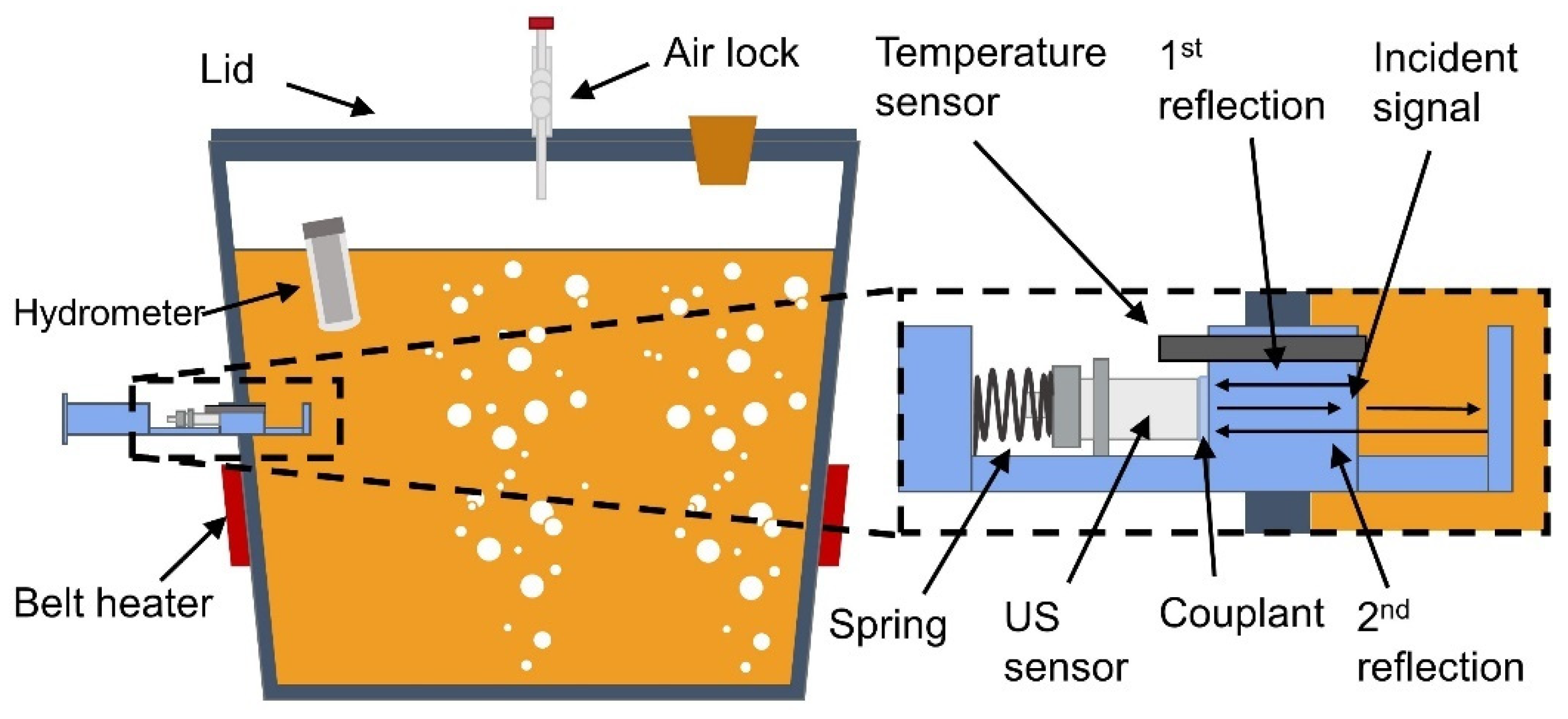
The fermentation was conducted in a 30 L cylindrical plastic vessel (Figure 1). A lid sealed the vessel to protect the wort from contamination. The lid contained an air lock to release the CO₂ produced during fermentation. A belt heater increased the temperature of the wort to facilitate fermentation. The wort was prepared in the vessel by dissolving and mixing 1.5 kg of malt (Coopers Real Ale, UK) and 1 kg of sugar (brewing sugar, the Home Brew Shop, UK) in 22 L of water. Once the ingredients were mixed, a US probe was installed, consisting of a US transducer (Sonatest, 2 MHz central frequency, UK) and a temperature sensor (RTD, PT1000, UK). The US transducer was connected to a Lecouer Electronique US Box (France) that excited the transducer and digitised the received US signal. The temperature sensor was connected to a Pico electronic box (PT-104 Data Logger, UK). The two electronic boxes were connected to a laptop that controlled the data acquisition. Coupling gel was applied between the US transducer and the probe, and a spring was used to maintain the contact pressure. A Tilt hydrometer was installed to provide real-time density measurements. The real-time density measurements were required as the ground truth data of the wort alcohol concentration to train the ML models. This device was a small cylinder that floats in the liquid with its centre of gravity different from its centre of buoyancy. This causes an inclination of the device that is dependent on the specific gravity of the fermenting media. The inclination of the hydrometer was measured by a self-contained accelerometer and was transmitted by radio to a smartphone located outside of the vessel. A calibration procedure related the inclination to the specific gravity. It should be noted hydrometers are not suitable for in-line monitoring of industrial fermentations. Firstly, the balance of the device can be easily distorted by foam or solids floating on the surface, or by bubbles produced during fermentation. Secondly, as the hydrometer floats on the wort surface, it would need manual removal at the end of each fermentation batch. The most accurate method of specific gravity measurement is to extract samples and use a portable density meter. However, this would require manual sample withdrawal at least every 2 h and would decrease the volume of liquid in the vessel, affecting the fermentation process. Furthermore, this would only produce sparse ground truth measurements of the density to train the ML models.

The yeast (Coopers Real Ale, UK) was distributed on the surface and the vessel sealed. The mixture was left for 4 to 7 days while the fermentation occurred. After this time, the fermentation equipment was cleaned and a new batch was prepared. In total, 13 batches were completed. During fermentation, data was collected from the three different sensors: the US sensor, the temperature sensor, and the hydrometer. The time of each measurement was also recorded. The fermentation batches were conducted over a period of approximately 3 months. This meant that the environmental and water temperature in the laboratory changed during this time. Furthermore, the belt heater was only in contact with the lower section of the vessel. This produced temperature variations from around 20 to 30 °C. However, this temperature variation is beneficial to our ML evaluation as each model must be able to generalise across a wide range of process temperatures.

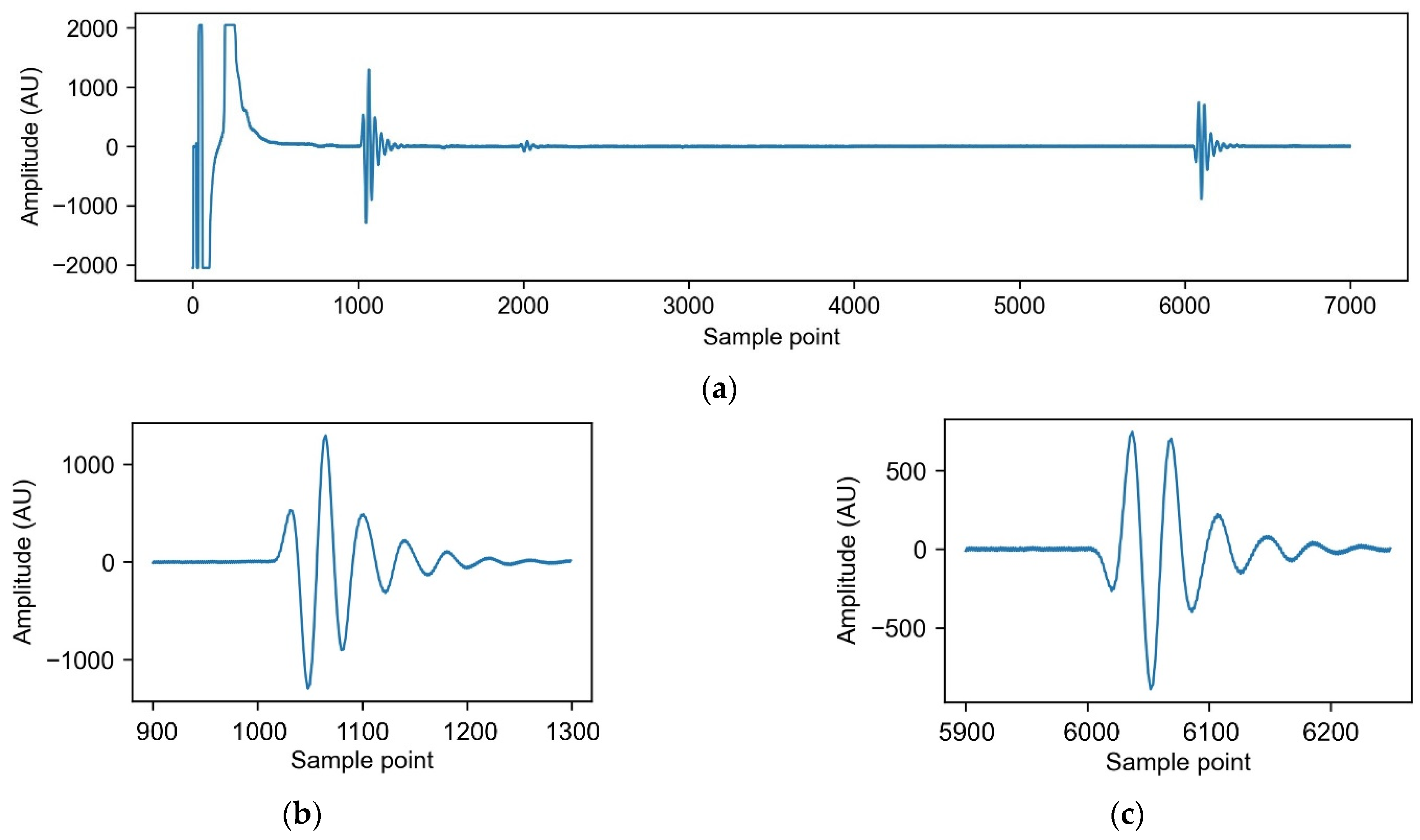
Sets of US and temperature data were collected periodically. Each of the sets consisted of 36 US waves and 36 temperature readings. For the US signal, 7000 sampling points were collected at 80 MHz sampling frequency. The time between each wave acquisition was 0.55 s. Between each set of data collection, 200 s elapsed. As depicted in Figure 1, the US transducers emitted sound waves which travelled along a PMMA buffer. At the interface between the buffer material and the wort, part of the sound wave is reflected back to the transducer (the 1st reflection). The rest of the sound wave continues through the wort, reflects at the opposite probe wall, and travels back to the transducer to be recorded (the 2nd reflection). An example of the signal recorded by the transducer is presented in Figure 2a. Close-ups of each reflection are presented in Figure 2b,c. The first section of the waveform (sample points < 500) is reflected back to the transducer before contacting the buffer material and wort interface and therefore contains no useful information about the process. The 1st reflection is identified between sample point 900 and 1500, and the 2nd reflection between 6000 and 6500, as shown in Figure 2.

2.1. Volume of Alcohol Calculation

The volume of alcohol (%) can be calculated from the specific gravity of the fermenting media using Equation (1) [27].

ABV = (SG_in − SG) × 131.25,

(1)

where ABV is the alcohol by volume (%), SG_in is the starting specific gravity of the liquid before the yeast was added, and SG is the current specific gravity of the fermenting liquid. The multiplier of this equation is based on the stoichiometric relationship of the fermentation reaction, where the decreasing density is due to CO₂ production and escape through the air lock [28].

2.2. Ultrasonic Wave Features

The following features were calculated from the obtained US waveform to use in the ML models. These are common features extracted from US waveforms [29]. The theory behind the selection of each feature is presented in their respective sections. Different combinations of these features were tested during ML model optimisation. The optimal feature combinations are presented in

Table 1. Results for the long short-term memory neural network (LSTM) models. MAE: mean absolute error; MSE: mean squared error; ABV: alcohol by volume. The regression metrics for the models evaluated on the test set are highlighted in bold at the bottom of the table.

Model	1	2	3	4
Reflections	1st and 2nd	1st and 2nd	1st	1st
Temperature	Yes	No	Yes	No
Optimal features	1st reflection energy 2nd reflection energy 1st reflection energy standard deviation 2nd reflection energy standard deviation Time of flight Temperature	1st reflection energy 2nd reflection energy 1st reflection energy standard deviation 2nd reflection energy standard deviation Time of flight	1st reflection energy 1st reflection energy standard deviation Temperature	1st reflection energy 1st reflection energy standard deviation 1st reflection peak-to-peak amplitude 1st reflection maximum amplitude 1st reflection minimum amplitude
Feature gradients	Yes	Yes	Yes	Yes
Batch size	2	2	4	4
Learning rate	0.01	0.01	0.033	0.033
LSTM units	2	2	4	4
L2 regularisation	0.0001	0.0001	0.00001	0.0001
Dropout rate	0	0	0	0
Epochs	100	100	100	100
Clip norm value	1	1	1	1
R2	0.952	0.939	0.878	0.948
MAE (% ABV)	0.265	0.355	0.426	0.283
MSE (% ABV)	0.136	0.173	0.345	0.146

, Section 3.1.

2.2.1. Energy

The waveform energy is a measure of the size of the waveform received by the transducer. For the 1st reflection, this is a measure of the proportion of the sound wave reflected from the interface between the buffer material and the wort. This is dependent on the change in acoustic impedance between these two materials [30]. Monitoring the waveform energy of the 2nd reflection offers additional information on the level of sound wave attenuation in the wort. This is caused by viscous losses in the media and scattering due to heterogeneities such as bubbles and yeast cells [30].

$$E={{\displaystyle \sum }}_{i=start}^{i=end}{A}_i{}^2,$$

(2)

where E is the waveform energy, A_i is the waveform amplitude at sample point i, and start and end denote the range of samples points for the reflection of interest [29].

2.2.2. Peak-to-Peak Amplitude, Maximum Amplitude, and Minimum Amplitude

The peak-to-peak amplitude, maximum amplitude, and minimum amplitude provide additional information as to how the energy is distributed in the waveform. Changes in wort composition or temperature may affect how the sound wave travels and reflects from boundaries, presenting differences in the shape of the received waveform. These three features were calculated for both the 1st and 2nd reflections.

PPA = max(A_start:end) − min(A_start:end),

(3)

A_max = max(A_start:end),

(4)

A_min = min(A_start:end),

(5)

where PPA is the peak-to-peak amplitude, A_max is the maximum amplitude, and A_min is the minimum amplitude.

2.2.3. Energy Standard Deviation

A total of 36 US waves were collected during each acquisition block. Phenomena in the process—e.g., the presence of bubbles at different times during fermentation—may cause fluctuations in the energy of the received waveforms. Therefore, the standard deviation of the energy in a block of acquired waveforms was investigated as a feature. The standard deviation of the energy was calculated for both the 1st and 2nd reflections.

$$STD=\sqrt{\frac{1}{W}{{\displaystyle \sum }}_{i=1}^{i=W}{\left(E_i-\overline{E}\right)}^2}$$

(6)

where STD is the standard deviation, W is the number of waveforms collected in the block, i is an individual waveform, and $\overline{E}$ is the mean waveform energy in the block.

2.2.4. Time of Flight

The time of flight was calculated using a thresholding method, i.e., the waveform sample point where the second reflection amplitude rises above the signal noise. This is a measure of the speed of sound in the wort that is dependent on its density and compressibility [20].

2.2.5. Feature Gradients

A one-sided, backwards moving mean was applied to obtain lagged feature representations over the previous 5 h. For the artificial neural networks (ANNs), this allows the use of past process information. For the long short-term memory neural networks (LSTMs), this allows for a way of storing past process information in some features, reducing the burden on the LSTM units to remember all feature trajectories.

2.3. Machine Learning

The ground truth data for the percentage volume of alcohol during fermentation was calculated from the portable density meter and hydrometer measurements. In total, 13 fermentation batches were monitored. The final two batches were selected as the test set to provide an unbiased assessment of the experimental methodology used. In an industrial setting, the final ML models would be deployed after collecting the training set runs. The remaining 11 batches were used in a 5-fold cross-validation procedure to optimize the ML models’ hyperparameters. Long short-term memory neural networks (LSTMs) are able to retain information from previous time-steps in a sequence. LSTMs are a type of recurrent neural network that reduces the likelihood of vanishing or exploding gradients by using gate units. This enables their use over much longer sequences [31]. To evaluate the utility of using LSTMs to predict alcohol concentration, they were compared with artificial neural networks (ANNs) which are unable to store past process information. ANNs combine input features to produce new features which can approximate the relationship with the target variable given enough neurons in the hidden layer [32,33].

For the LSTMs, zero-padding was applied to the US features to make every fermentation batch sequence an equal length. A masking layer specified that the LSTM units ignore this padding. Each sequence consisted of 4646 timesteps. All timesteps for each batch were used as a single sequence rather than being split into multiple sequences of shorter length. While long LSTM sequences (250–500 timesteps) are prone to produce vanishing gradients when predicting a single output, this is not a problem when predicting an output at every timestep as used in this task [34].

For the ANNs, a single hidden layer and the Adam optimisation algorithm was used. Cross-validation determined the optimal batch size, number of neurons in the hidden layer, learning rate, drop-out rate, L2 regularisation penalty, and number of epochs for training. For the LSTMs, the Adam optimisation algorithm was used and the cross-validation procedure determined the optimal batch size, number of LSTM units, learning rate, drop-out rate, L2 regularisation penalty, gradient norm clipping value, and number of epochs. After cross-validation, the set of hyperparameters which resulted in the lowest average validation error were used to train a final model using all of the training set. The networks were trained using TensorFlow 2.3.0. The coefficient of determination (R²), mean squared error (MSE) and mean absolute error (MAE) were used as performance metrics to evaluate the ML models. Multiple metrics produce a comprehensive assessment of a model’s ability to fit to the test set and improve comparison between models.

3. Results

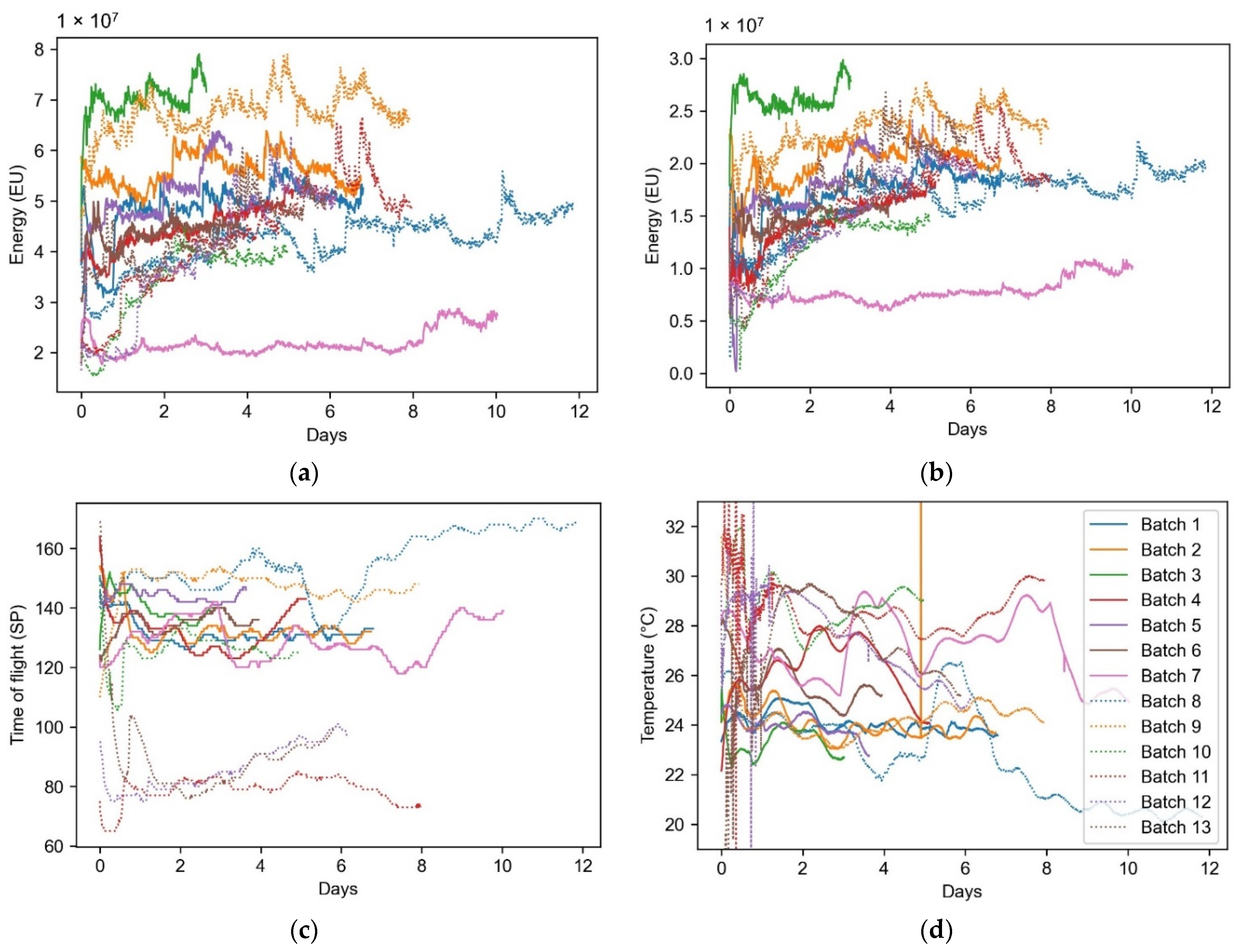
Figure 3 displays selected features from all the fermentation batches. It is shown that the energy of 1st reflection (Figure 3a), energy of the 2nd reflection (Figure 3b), and the time of flight of the sound wave through the wort (Figure 3c) start at different values for each batch. There are several explanations for this. Firstly, as presented in Figure 3d, the process temperature is not the same at the start of each batch. As the speed of sound is highly dependent on temperature, the US properties begin from different magnitudes. Secondly, the US probe required manual removal and repositioning when disposing each batch after fermentation. This disturbed the spring maintaining the contact pressure of the US transducer, which affects the sound energy transferred through the materials from the sensor.

The trajectories of the waveform features are also not smooth. Again, this is partly due to the oscillating process temperature. In addition, bubbles of CO₂ produced during the fermentation were observed to attach to the surface of the probe material, which would cause scattering and reflection of the sound wave. During the fermentation, as further CO₂ bubbles were produced, the new bubbles would replace the previous ones on the surface. This is likely to cause fluctuations in the waveform energy transferring through the interface between the probe and the wort.

The energy of the 1st reflection increases throughout the fermentation (Figure 3a). The energy of the 1st reflection is proportional to the change in acoustic impedance at the buffer-wort interface, with the acoustic impedance being a product of the material density and speed of sound [20]. As the density of the wort decreases during fermentation, the speed of sound also decreases as found in [17,18,35]. As the solid buffer material has a greater density and speed of sound than the starting wort, the proportion of sound wave reflected at the buffer-wort material increases throughout the fermentation. However, the time of flight (Figure 3c), the inverse of the speed of sound, shows no general trend. This contrasts with the results obtained in [17,18,35], which suggests that it should increase. This is likely due to the changing process temperature masking an increasing time of flight. The results in [17,18,35] were all obtained at a constant temperature. The reduced time of flight for the last three batches (Batches 11, 12, and 13 in Figure 3c) is most likely due to a disturbance of the sensor positioning after Batch 10. These batches were kept in order to provide an unbiased assessment of the experimental methodology used. In an industrial setting because the test set data (batches 12 and 13) would not be available to analyse prior to the ML model training. The energy of the 2nd reflection is diminished compared with the 1st reflection at the beginning of the fermentation until approximately Day 3, as presented in Figure 4. A similar result was found in [17] and is due to the fermentation being most vigorous at the start of the process. This causes more CO₂ bubbles to be produced and therefore greater attenuation of the sound wave travelling through the wort.

3.1. Machine Learning

The ANN model with the highest accuracy only achieved an R² of 0.398 (MAE = 1.010% ABV, MSE = 1.942% ABV). As such, only results from the LSTM models are included in Table 1. This shows that the gradients of the features, as provided to the ANNs, is insufficient, and the enhanced memory of the feature history provided by the LSTM units is required for this process. 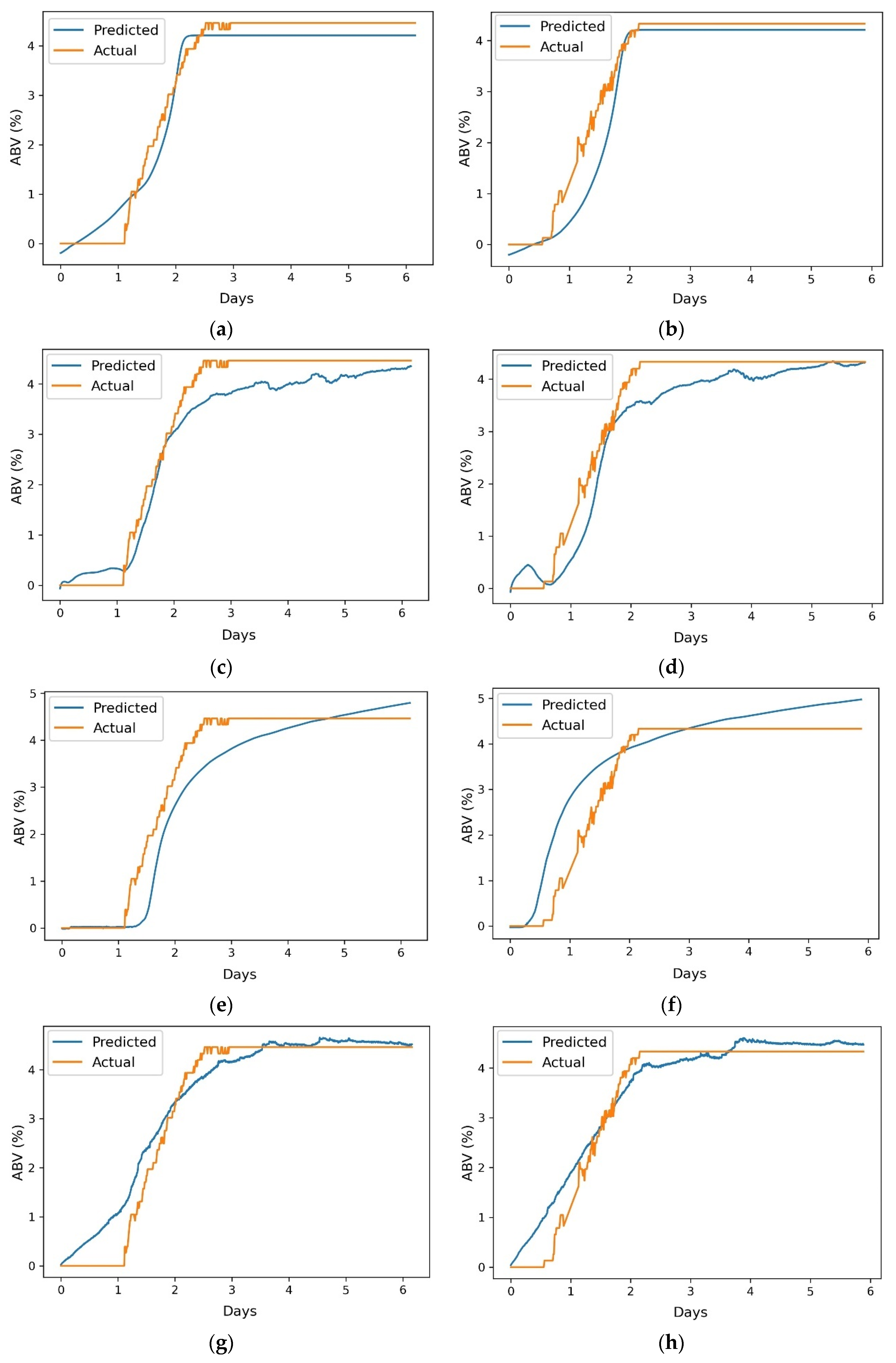The results of four final LSTM models are presented in Table 1, which either use the 1st reflection or both reflections, and either use the temperature as a feature or not. The optimal features, optimal hyperparameters, and performance metrics are included. The most accurate LSTM model (Model 1) used features from both the 1st and 2nd reflections and the process temperature. Interestingly, the second most accurate model (Model 4) only used features from the 1st reflection, excluding the process temperature. The third most accurate model (Model 2) used features from the 1st and 2nd reflections without the process temperature. Finally, the least accurate model (Model 3) combined features from the 1st reflection and the process temperature. Graphical representations of these predictions are shown in Figure 5a–h.

4. Discussion

The most accurate model (Model 1) uses features from both the 1st and 2nd reflections and the process temperature. This shows the potential of US sensors to predict the endpoint of fermentation and, as demonstrated in Figure 5a,b, accurately predict the alcohol concentration throughout the fermentation process. However, industrial implementation of this model would require the use of an invasive probe in order to obtain the 2nd reflection. In addition, an invasive temperature probe would be required to monitor the changing temperature of the fermentation media. Interestingly, the second most accurate model (Model 4) only used features from the 1st reflection and excluded the process temperature. The use of only the 1st reflection indicates that accurate results could be obtained using a non-invasive, no-transmission US sensor, similar to the techniques used in previous works by our group [23,24,25,26]. This is advantageous as it allows the alcohol volume to be accurately predicted by easily mounting a US sensor externally to an existing vessel. Therefore, it can be easily implemented into existing industrial settings at low effort and cost. The use of Model 4 would also remove the requirement for an invasive process temperature measurement. Furthermore, the performance metrics for Model 4 (R² = 0.948, MAE = 0.283, MSE = 0.146) are similar to those of Model 1 (R² = 0.952, MAE = 0.265, MSE = 0.136) indicating that no prediction accuracy would be lost through using a non-invasive and no-transmission sensor approach. This US sensing technique would also not require a hole to be bored into the vessel side, as used in this work. Instead, the US wave could be transmitted through the vessel wall.

In Model 3, the features from the 1st reflection combined with the process temperature produces a reduced accuracy. This is likely because the additional features required in Model 4 (the peak-to-peak amplitude, maximum amplitude, and minimum amplitude of the 1st reflection) contained more pertinent information about the temperature at the probe-wort interface than the non-local temperature sensor. The suggestion that the temperature sensor measured the temperature of the bulk wort instead of the region through which the 1st reflection passes is supported by the results from Model 2. When the temperature was removed as a feature, Model 2 produced a reduced accuracy compared with Model 1. This indicates that for accurate prediction using the 2nd reflection, the bulk wort temperature measurement is required as the sound wave travels through this region. The reduced accuracy obtained when combining the temperature data with the 1st reflection for Model 3 is most likely caused by the temperature at the probe-wort interface not closely following the trend of the bulk wort temperature. Therefore, using the temperature measurement as a feature increases the model complexity with little benefit, meaning it is more difficult for the network to find an optimal solution. This further supports the aforementioned point that accurate, invasive temperature measurement would not be required with a non-invasive, no-transmission US sensing technique.

Figure 5 displays the predicted ABV percentage from the trained LSTM models for the two batches used for the test set (batches 12 and 13). Model 1 (Figure 5a and b) accurately determines the fermentation endpoint. However, the final ABV prediction is not as accurate as Model 4, indicating that it may not be sensitive enough to determine differences in final ABV between batches. Whilst Model 3 appears to have no utility, Models 1, 2, and 4 all accurately followed the ABV trajectory. Owed to the real-time data acquisition of US sensors, these models suggest that the obtained data could be used to train additional anomaly detection models to provide early warning of undesired process trajectories within a batch.

Several locations in the prediction require improvement; for example, the detection of ABV plateau for Model 2 (Figure 5c,d around the 2nd day), the settling at a final ABV for Model 3 (Figure 5e,f), and the detection of the initial ABV rise for Model 4 (Figure 5g,h around the first day). This is likely due to the varying temperature throughout the fermentation having a large effect on the US properties of the wort compared with the changing density. There are also locations of decreasing ABV prediction (Figure 5d during the first day) or sudden increases in ABV prediction (Figure 5h at the end of the fourth day). This is likely due to the temperature variations being different for each batch and the particular temperature variations during the test set causing these effects. These problems would likely be reduced through obtaining more training data.

In this work, ML models were trained to predict the ABV throughout the fermentation. However, in industrial settings this may not be the most appropriate output value with which to fit a model. For example, ML models could be trained to predict the final ABV of each batch, the time remaining until the ABV plateaus, classify the end of fermentation, or provide early detection of anomalous batches. In each of these cases, the models would be trained for a more specific purpose, as such the models may perform better than indicated by Figure 5. This work is therefore demonstrative of the efficacy of real-time fermentation monitoring using US sensors and ML, and increased accuracy may be achieved through predictions of more specific outputs.

If only the 1st reflection was used in an industrial monitoring system, the sound wave could be transferred through the vessel wall. Alternatively, if the 2nd reflection was also to be used, the probe could be fitted through existing ports common to industrial fermenters. This work monitored a laboratory scale fermentation process. At industrial scale, agitation methods are uncommon in beer fermentation to prevent damage to the yeast [36]. Therefore, radial variations in alcohol concentration exist and there would be a difference in the alcohol concentration at the sensor measurement area and the bulk wort [36]. However, previous work from our group showed that a non-local probe could accurately monitor a mixing process [23]. This is because, through machine learning, the sensor data is correlated to the location of the ground truth data, rather than the sensor. In this case, a sensor would be trained to predict the alcohol concentration at the location of the hydrometer measurements or sample collection.

Future Research Directions

The largest barrier to industrial implementation of sensors and ML combined technologies is the burden of obtaining labelled data. Labelled data is used as the targets for training supervised ML models. To obtain the ground truth to label data requires another analysis method. In this work, the hydrometer readings were used due to the sample density measurements producing insufficient data points and disturbing the fermentation. In an industrial setting, the hydrometer may only be able to be used for a small number of batches for ML model development. In this case, semi-supervised learning may be required to train high accuracy models. Semi-supervised learning uses both labelled and unlabelled samples to train a model [37,38,39]. Firstly, unsupervised learning techniques, such as principal component analysis or autoencoders, can be used on the total dataset to learn relationships between features across the labelled and unlabelled samples. Then traditional supervised learning can be used on the new features using just the labelled samples. Secondly, a self-training (or pseudo-labelling) approach may be used to predict the labels of the unlabelled data from the trained model. These pseudo-labels may then be added to the labelled data set and the procedure repeated to improve the label predictions or to train a final model.

Alternatively, conventional sample extraction and density measurement may be used to obtain the labelled data. Either a curve may be fitted to these sparse density measurements to produce interpolated data points, or a similar semi-supervised learning procedure can be implemented. Active learning may also be used to identify data points for labelling that may be the most useful to the model [40,41]. These datapoints may be during a sparsely sampled time in the fermentation or be in a particular temperature and composition range. Operators could then analyse these samples to provide the most benefit to the ML model at the lowest investment in effort.

5. Conclusions

The transition to Industry 4.0 promises increased manufacturing efficiency, sustainability, and productivity. By implementing digital technologies such as the Internet of Things, Cloud Computing and ML, not only can entire processes be integrated, but supply chains as well. Sensors are a key technology in this revolution by providing the real-time data to inform automatic, intelligent decision-making. Currently, beer fermentation is monitored through periodic manual sampling and off-line wort density measurements. This work has presented an in-line, low-cost US sensing technique combined with ML, which would remove the need of operator sampling. This work has shown that US sensor data combined with LSTM models are able to accurately predict the volume of alcohol during beer fermentation. The highest accuracy model (R² = 0.952) used a transmission-based ultrasonic sensing technique along with the process temperature. Importantly, the second most accurate model (R² = 0.948) only used a reflection-based technique without measurement of the temperature. This demonstrates the potential for a non-invasive, no-transmission US technique, which doesn’t require invasive measurement of the process temperature. This sensing technique could be easily and inexpensively retrofitted onto existing fermentation vessels.