Article

Optimal Control Applied to Oenological Management of Red Wine Fermentative Macerations

by
Ricardo Luna
1,
Bruno M. Lima
2,3,
José Cuevas-Valenzuela
1,
Julio E. Normey-Rico
2 and
José R. Pérez-Correa
3,*
1
Center for Research & Innovation (CRI), Viña Concha y Toro, Pencahue 3550000, Chile
2
Department of Automation and Systems, Federal University of Santa Catarina, Florianópolis, Santa Catarina 88040-900, Brazil
3
Department of Chemical and Bioprocess Engineering, Pontificia Universidad Católica de Chile, Santiago 7820436, Chile
*
Author to whom correspondence should be addressed.
Submission received: 29 April 2021 / Revised: 29 May 2021 / Accepted: 31 May 2021 / Published: 10 June 2021
(This article belongs to the Special Issue Control of Wine Fermentation)

Abstract

:
The management of wineries for industrial red winemaking is limited by the capacity and availability of fermentation tanks over the harvest season. The winemakers aim to optimize the wine quality, the fermentative maceration length, and the fermentation tank’s productive cycle simultaneously. Maceration in varietal wine production is carried out until a specific sugar content (digging-out point) is attained, finishing before alcoholic fermentation. Winemakers have found that by trial and error handling of the digging-out point, they can improve the winery capacity and production cost. In this work, we develop an optimal control problem for managing the digging-out point considering two objectives associated with process efficiency and costs. A good compromise between these objectives was found by applying multi-criteria decision-making (MCDM) techniques and the knee point. Two control strategies were compared: free nutrition and traditional nutrition. TOPSIS and LINMAP algorithms were used to choose the most suitable strategy that coincided with the knee point. The preferred option was nitrogen addition only at the beginning of fermentation (6.6–10.6 g/hL of DAP) and a high fermentation temperature (30 °C), yielding the desired digging-out point with a small error (6–9 g/L).

1. Introduction

In red winemaking, the must is fermented in contact with grape pomace and seeds to extract several phenolic compounds, such as anthocyanins and tannins, which define the color and mouthfeel properties of red wine, respectively [1]. This process is known as fermentative maceration and generally begins with the grape crushing process [2]. The extraction kinetics of these phenolic compounds depend on several variables, such as the solid–liquid phase’s contact area, their molecular structure (skins and seeds), maceration duration, temperature, and solvent composition [3]. Therefore, the way in which the alcoholic fermentation is performed is a significant factor contributing to wine quality.
At industrial-scale wineries, only some of these variables can be controlled. The fermentation temperature is usually controlled by a closed-loop control manipulating the refrigerant’s flowrate that circulates through the tank’s jacket. Winemakers control phenolic extraction, comprising homogenization of must and skins, by defining the maceration duration and the pump-over program. The maceration process finishes when the solids are separated from the fermenting juice, known as the digging-out point. Overall, winemakers define this as the point at which a specific sugar content or must density is achieved. This criterion is handled through wine taste, wine color, grape quality, and the management of the winery capacity.
The operation strategy should be adapted season to season to the uncertainties and vintage shortening caused by climate change [4]. Global warming has led to problems in the planning, management, and productivity of the winery. In particular, the winery’s management is limited to the fermentation tanks’ capacity and availability on a specific date. Consequently, winemakers frequently change the original fermentation recipe and make new decisions during the fermentation, such as reducing the maceration duration or increasing the fermentation rate by adding diammonium phosphate (DAP). Optimal handling of maceration and DAP additions could improve wineries’ capacity and reduce production costs without sacrificing the wine’s quality and typicity.
Model-based design (MBD) and model predictive control (MPC) can achieve optimal fermentation operating strategies that simultaneously optimize efficiency, economic indexes, and product quality. The winery operation can be adapted to unexpected events during the vintage season by applying these techniques, providing faster and more reliable solutions than experimental trial and error [5]. The process model’s reliability and predictive capacity are crucial to guarantee the robust performance of these techniques.
Most wine fermentation models are described by a set of nonlinear differential and algebraic equations (DAEs) with specific assumptions and purposes [6]. Coleman et al. [7] developed a simple lumped parameter model assuming nitrogen as the primary limiting substrate and temperature-dependent kinetic parameters. Cerda-Drago et al. [8] considered a spatial distribution to describe oxygen incorporation and dissolution during white wine fermentation. Zenteno et al. [9] developed a compartment model to simulate the temperature gradients at an industrial scale. Miller et al. [10], Miller et al. [11] developed a three-dimensional industrial red wine fermentation model using the finite element method to simulate the temperature gradient and their influence on anthocyanin and tannin extraction rates.
The above studies focused on replicating experimental fermentations operating under similar conditions. New operating conditions are rarely explored by optimization techniques. Model-based design could allow exploration of the impact of new operating conditions such as fermentation temperature profile or nutrient addition during fermentation. Overall, MPC has been applied widely in the pharmaceutical and biochemical industries: penicillin production [12], bacterial culture for acetate production [13], mammalian cell culture for glucose production [14], and fed-batch ethanol production [15]. Nevertheless, the applications of MPC to fermentation tanks in the wine industry are scarce. Schenk et al. [16] developed an MPC to minimize the cooling energy in white wine fermentation. The MPC strategy reduced the energy consumption by 52% compared to an industrial controller without decreasing the wine quality.
Model-based optimal operation has been increasingly applied in the process industries since the arrival of the Industry 4.0 paradigm [17]. The higher levels of automation and digitalization allow mathematical models to transform process data into valuable information for online automatic high-level decision-making [18]. The beverage and food industry has adopted these technologies (sensors, big data, machine learning models, first-principles models, etc.) at a slower rate than other process industries such as mineral, chemical, and pharmaceutical production plants [19]. To the best of the authors’ knowledge, the application of MPC and the development of optimal strategies for industrial red wine fermentation have not been tackled yet. There are very few applications of model-based optimal decision-making in the alcoholic beverage industry. For instance, Rodman and Gerogiorgis [20] applied dynamic multi-objective optimization (MOO) to the beer fermentation process. The optimization problem looked for an optimal temperature profile that could simultaneously maximize the final ethanol concentration and minimize the fermentation time. Luna et al. [21] solved a dynamic MOO problem to design optimal distillation recipes for muscat wine spirits. Moreover, they used multi-criteria decision-making (MDCM) algorithms to select different kinds of muscat spirit recipes based on objective prioritization. These applications demonstrated that model-based optimal operation and MDCM techniques could be valuable tools for managing the wine process.
Hence, our hypothesis is that using model-based optimal control and MCDM techniques makes it possible to improve the process efficiency and costs compared with standard operation, without sacrificing product quality. In this work, an optimal control problem (OCP) for red wine fermentation is developed using a reparametrized fermentation kinetic model [22]. The OCP considered two oenological objectives: i) sugar target concentration at the digging-out point and ii) minimization of the total DAP additions throughout fermentation. The decision variables were the fermentation temperature profile and the DAP addition during the fermentative maceration. A dynamic MOO problem was formulated and solved by applying the weighting approach. Two nutrition strategies were evaluated: free nutrition at each sampling time and traditional nutrition that considers two additions, one at the beginning and another at the middle of the fermentation process. Then, the optimal strategies were selected using MCDM algorithms. Thus, the main contributions of this work are:
  • Optimal control for managing industrial bulk red winemaking;
  • Weighting approach for solving MOO problems with oenological requirements;
  • MCDM algorithms for helping the decision-making process.
The paper is organized as follows: a brief process description for industrial bulk red winemaking is introduced in Section 2.1, where the digging-out point is defined as the separation of the solids from the fermenting must at the specific sugar content. A general explanation of the dynamic fermentation model is introduced in Section 2.2. The oenological multi-objective cost function using the weighting approach is detailed in Section 2.3. The optimal control problem formulation and the nutrition strategies are presented in Section 2.4. The MCDM algorithms and the knee point are introduced in Section 2.5. Finally, the results and the conclusions are presented in Section 3 and Section 4, respectively.

2. Materials and Methods

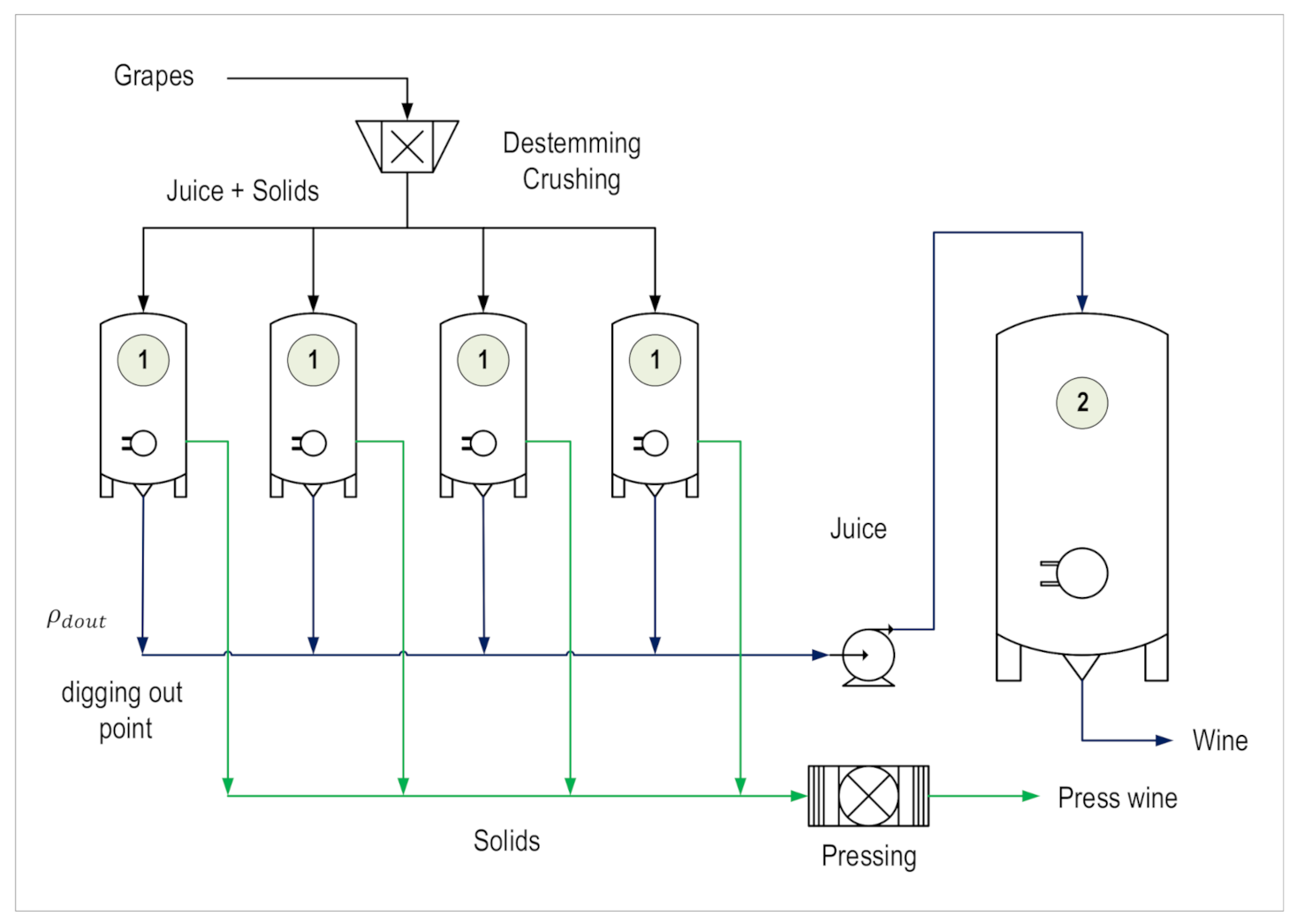
2.1. Process Description

Red wine fermentation involves simultaneous fermentation and solid–liquid extraction (maceration); hence, it is also called fermentative maceration. In commercial wineries, the maceration duration is typically regulated to achieve a specified level of phenolics. Short macerations are preferred for varietal or bulk wines, while longer macerations (extended macerations) are favored for premium wines [23]. Since our technology is intended to produce varietal red wines, we focus on shorter macerations, which finish before the fermentation is completed. Figure 1 shows the process scheme for industrial red winemaking for bulk wines. The process is divided into fermentative maceration (FM) and fermentation completion (FC). The FM stage is carried out in first set of tanks until the digging-out point is reached, where the specific sugar content is achieved; this is called digging-out density by winemakers. At this point, the solids are separated from the fermenting must, and the liquids from the different tanks are transferred into a larger tank to complete the fermentation. In this study, we developed a model-based procedure for the optimal management of the digging-out point in FM.

2.2. Fermentation Model

The kinetic fermentation model developed by Zenteno et al. [9] was used to design the optimal operation strategies. The model was simplified by removing the compartment equations; hence, temperature gradients were not considered [22]. The nitrogen addition and temperature setpoint were added as model inputs since they are the decision variables of the formulated optimal control problem. The C O 2 state variable was removed from the model since it did not affect other state variables. The model equations are represented represented by Equation (1):
d x d t = f x ( t ) , u ( t ) , θ ρ ( t ) = h G ( t ) , F ( t )
where x, u θ , and t correspond to the state variables, model input vector, model parameters vector, and time process, respectively. The state variables are biomass ( X ) , nitrogen ( N ) , glucose ( G ) , fructose ( F ) , and ethanol ( E ) . Total sugar ( S ) includes glucose and fructose. Table 1 shows the initial values of the state variables. The model inputs ( u ) are the nitrogen addition using DAP ( N d a p ) and the fermentation temperature ( T ) . The model parameters ( θ ) were estimated using a specifically designed, robust reparameterization method for red wine fermentation [22], which yields an optimal model structure characterized by given free and fixed parameters. The model parameter values and model equations are available in Torrealba et al. [22] and Zenteno et al. [9], respectively. Finally, ρ corresponds to the must/wine density and was calculated through a correlation with total sugar (S) obtained using experimental fermentation data. The complete model equations are given in Appendix A.

2.3. Multi-Objective Cost Function

The objective function Equation (2) considers the process efficiency and costs during fermentative maceration. The process efficiency is associated with oenological requirements, such as the sugar level at the end of the fermentative maceration stage (digging-out point; see Section 2.1). The amount of DAP added at the beginning and during fermentative maceration defines this stage’s operating costs. The optimal control is formulated as the following MOO problem:
min u i J ( u i ) = α · S ( t d o u t ) S s p 2 100 + ( 1 α ) · i = 1 n N d a p , i 0.200
where α is a relative weight (positive scalar 1 ) defining the objective’s priority and N d a p , i is the nitrogen added at time i considering a sample time of 6 h. This approach is known as the weighting method, which transforms the MOO into a traditional single-objective problem [24,25]. The first objective is to obtain the desired sugar concentration at the digging-out point. Here, S s p is the sugar setpoint defined by the winemaker at the digging-out point, and t d o u t is the digging-out time. In this study, the digging-out point is established as five fermentation days ( t d o u t = 120 h) with S s p = 11 g/L of sugar concentration (equivalent to 995 kg/m 3 ). The second objective is the minimization of the total nitrogen addition over a time period of t = 120 h (see Section 2.4).
Both objectives were normalized to obtain comparable values. The sugar setpoint weight was defined by trial and error, and the second term weight (1/0.200 g/L) corresponds to approximately the maximum DAP dose allowed by the Chilean law (96 g/hL), considering that it is composed of 21% nitrogen [26]. Finally, grid values for alpha were defined to solve the MOO problem ( α = [ 0 , 0.02 , 0.04 , , 1 ] ), resulting in 51 optimization problem runs.

2.4. Optimal Control Problem Formulation

The optimal control problem (OCP) searches the manipulated variable profile (nitrogen addition, fermentation temperature) that minimizes the objective function and satisfies the constraints. The optimization problem was discretized using a direct collocation method, which simultaneously solves the simulation and optimization [27]. This method discretizes the control and state variables over a time period, using collocation points on finite elements [28]. Then, the OCP was reformulated as a nonlinear programming problem (NLP) [27,29] by Equations (3):
min u i J ( u i ) s . t i = 1 n , j = 1 m x i , j = x i 1 + h i j = 1 m Ω j ( τ j ) · d x d t i , j d x d t i , j = f ( x i , j , y i , j , u i , j , θ ) g ( x i , j , y i , j , u i , j , θ ) = 0 u L u i , j u U , x L x i , j x U , y L y i , j y U
where n is the number of finite elements, m is the number of collocation points, h i is the length of the finite element (sample time), and Ω is the interpolation polynomial function for each finite element. In total, 20 finite elements over a time period of 120 h (finite element size was t i = 6 h) and five Legendre collocation points were used. In this equation, x, y, u, and θ correspond to the state variables, algebraic variables, control variables, and model parameters vector, respectively. The simultaneous simulation/optimization problem was coded in Python using the CasADi package [30] with the optimization solver IPOPT [31].
Two control strategies were compared. One considers the fermentation temperature variation and nitrogen additions at each sampling time ( t i = 6 h) as decision variables. This strategy has more degrees of freedom, and we called it free nutrition (FN). The second strategy, called traditional nutrition (TN), considers temperature variation at each sample time, but with only two nitrogen additions: at the beginning of the process (t = 0 h) and at t = 48 h, which corresponds to the start of the yeast stationary growth phase (1070–1050 kg/m 3 ) [32,33]. In both cases, the fermentation temperature path was constrained to the range of 20–30 °C while total nitrogen addition should be lower than 0.200 g/L.

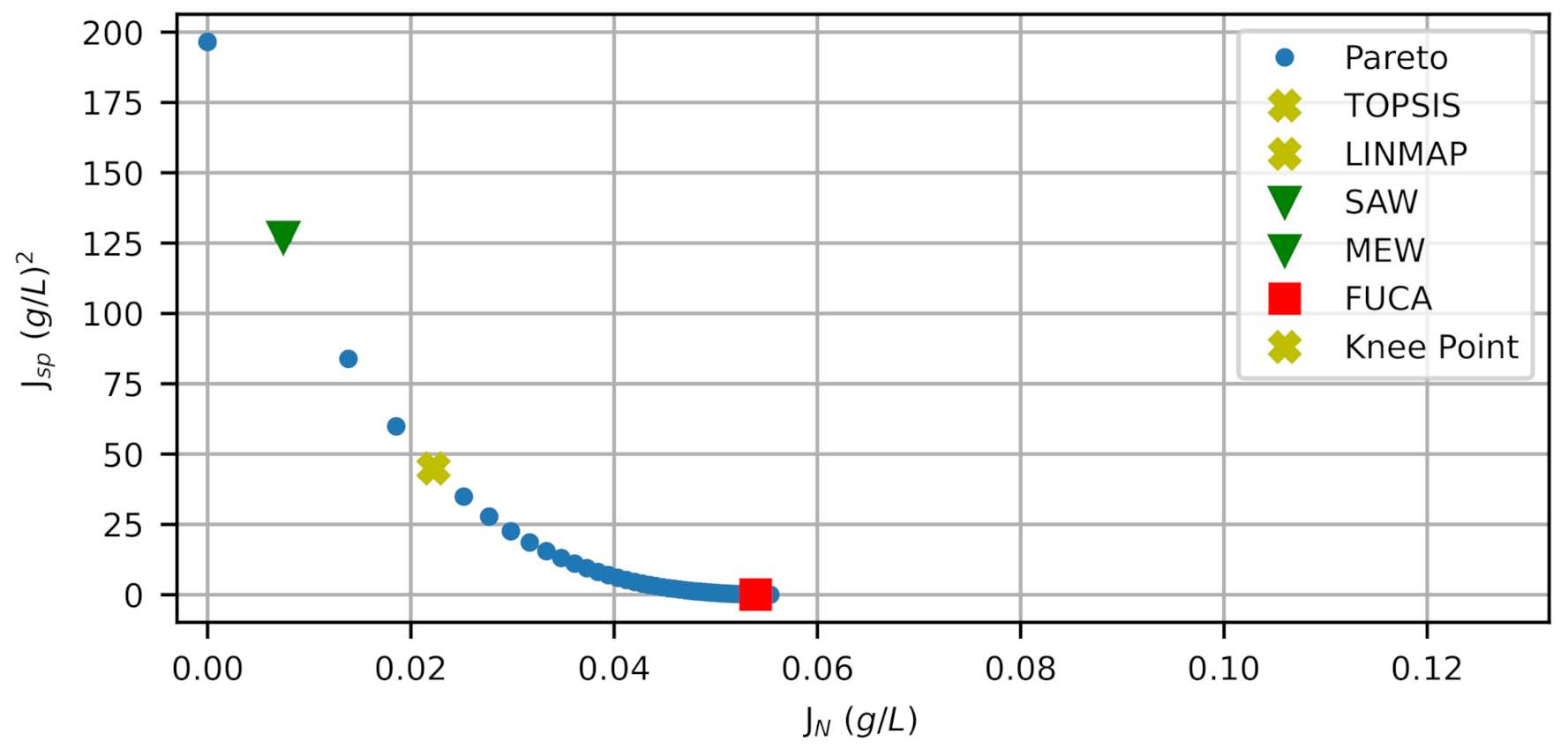
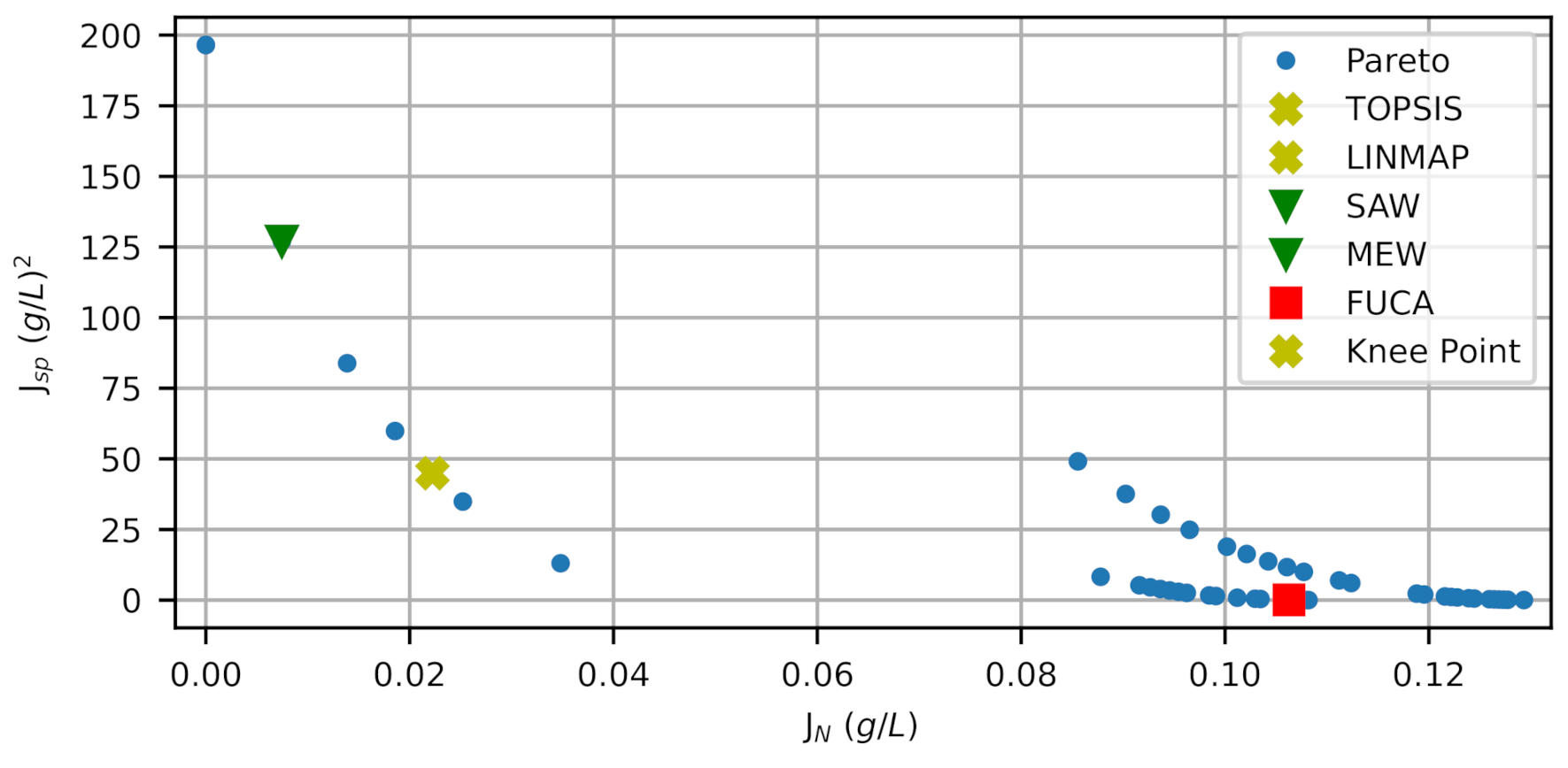
2.5. Selection of Optimal Control Strategy by MCDM

The solution of the MOO problem is a set known as non-dominated solutions or Pareto front, which is represented as an objective matrix (f) with n rows (one row for each Pareto solution) and m columns (one column for each objective). Here, the dimension of the objective matrix was n = 21 and m = 2 (see Section 2.3). The next step is to select one of the non-dominated solutions, and multi-criteria decision-making (MCDM) algorithms have been developed for this purpose [34]. In this work, simple MCDM algorithms were evaluated to select an optimal solution: TOPSIS, LINMAP, SAW, MEW, and FUCA. These algorithms require a weight (w) for each objective defined by the user. For this application, a compromise among the objectives is needed. These solutions are known as “knee” points, where a significant improvement in some objectives means insignificant degradation in the other objectives [35,36]. Therefore, the weights of the MCDM algorithms were set with equal priority ( w = [ 0.5 , 0.5 ] ) for both objectives. Moreover, the optimal solutions selected by the MCDM algorithms were compared with the knee point to evaluate the performance. The knee point was calculated as the minimum Euclidean distance between each optimal solution ( d i ) and the utopian solution by Equations (4) and (5):
F i , j = f i , j max i n ( f i , j )
d i = j = 1 m F i , j F j * 2
where F i , j is the normalized objective matrix and F j * are the coordinates of the utopian solution for each objective. Since both objectives correspond to a minimization criterion, the utopian point was zero ( F 1 , 2 * = [ 0 , 0 ] ). The solution with the smallest d i is the knee point.

3. Results

This section presents the obtained results and it is divided into three parts: (i) the free nutrition case study; (ii) the traditional nutrition case study, and (iii) comparative results of the most suitable strategies.

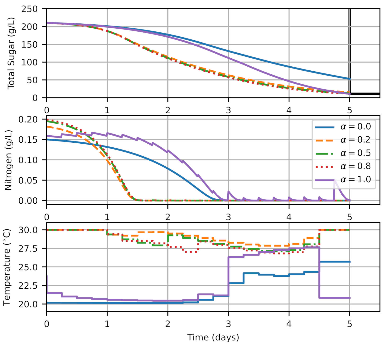
3.1. Free Nutrition Strategies

The simulations of optimal control for free nutrition strategies are shown in Figure 2 for different values of α . As expected, the strategy for α = 0 (priority for minimization of nitrogen additions) did not add any DAP, but the sugar level at the end of the maceration process was far from the desired digging-out point (42 g/L sugar difference). On the other hand, the strategy with α = 1 achieved the sugar concentration of the desired digging-out point by the end of the maceration, and DAP was added at each sampling time, obtaining 94.3 g/hL of total DAP dose (near the limit). Overall, the fermentation temperature profile was low for both strategies for the first three days and then increased near the end.
Intermediate α values (0.2, 0.5, 0.8) yielded similar strategies, characterized by nitrogen additions concentrated at the beginning of the fermentation with DAP doses of 15, 22, and 25 g/hL, respectively. Moreover, the sugar differences from the desired digging-out point were small, namely 4.3, 1.45, and 0.43 g/L, respectively, representing an error smaller than 5%. In all cases, temperature profiles throughout the fermentation were characterized by high values (>27 °C).
Figure 3 shows the Pareto front composed of 51 solutions, the selected solutions by MCDM, and the knee point. The solution chosen by TOPSIS and LINMAP was the same and coincided with the knee point. These algorithms are very similar and usually recommend similar or the same solution [21,34]. This optimal solution corresponds to the strategy with α = 0.08 . SAW and MEW are also similar approaches that often recommend the same solution [21,34]. Here, the solution chosen by SAW and MEW is the neighbor of the knee point ( α = 0.06 ). This solution added 3.6 g/hL of DAP at the beginning of the fermentation, and the error from the digging-out point was 11.3 g/L. Finally, the FUCA method selected a solution ( α = 0.02 ) far from the knee point that prioritizes the minimization of nitrogen additions (0 g/hL of DAP) with 14 g/L of sugar difference from the desired digging-out point.

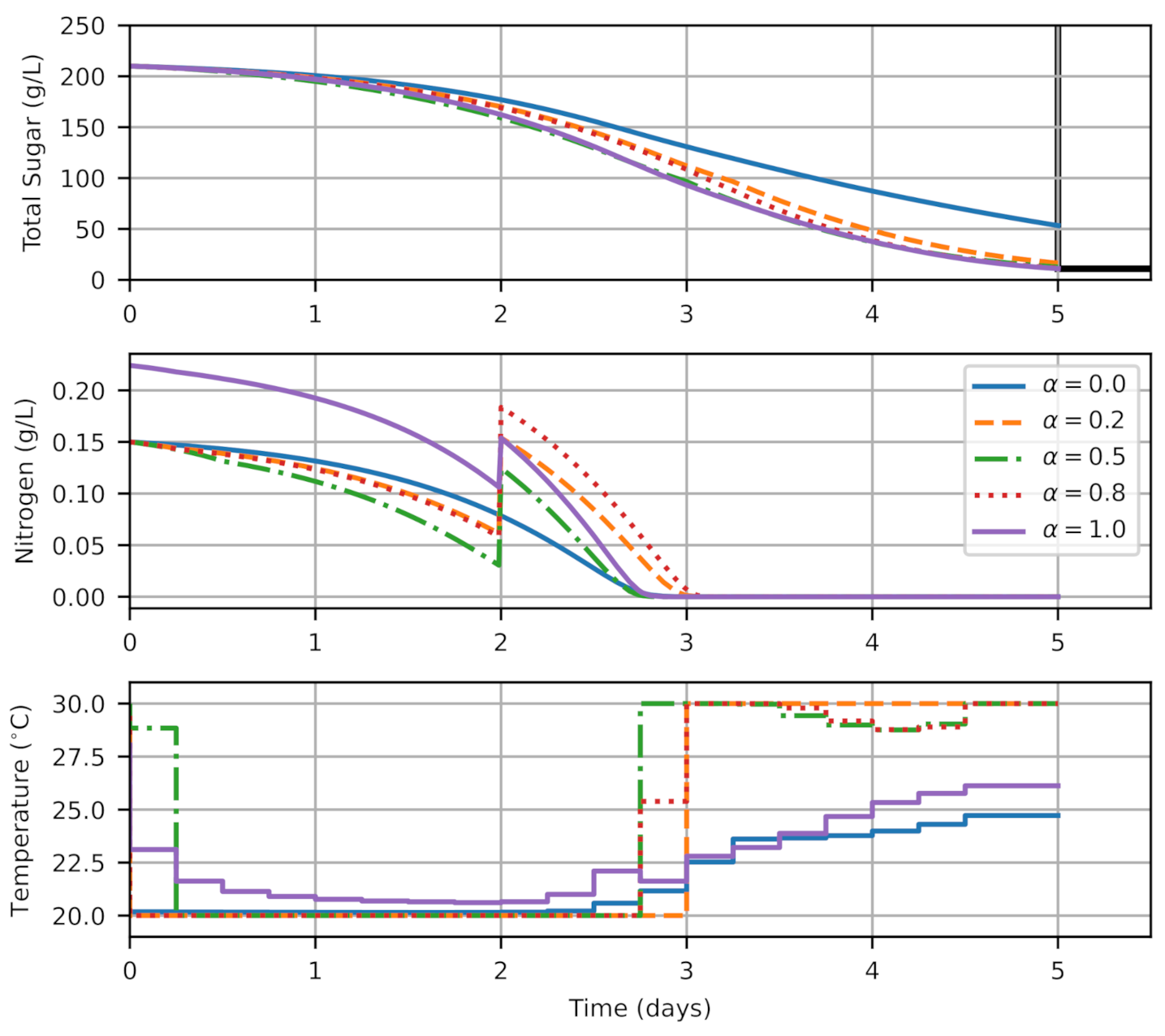
3.2. Traditional Nutrition Strategies

Figure 4 shows the simulation of optimal control for traditional strategies for different values of α . Like the FN strategy, the TN strategy for α = 0 did not add DAP and the sugar concentration achieved was 53.4 g/L, i.e., 43.4 of sugar difference from the desired digging-out point. Contrarily, the TN strategy with α = 1 achieved the desired digging-out point (11 g/L of sugar), and the total DAP addition was 58.7 g/hL, where 35.3 g/hL was added at the beginning and 23.4 g/hL at time t = 48 h. For both TN strategies, the temperature profile was very similar. For the first 2.5 days, the temperature was low (near the lower bound 20 °C) and then linearly increased to 25 °C.
Contrarily to the FN strategies with α values 0.2, 0.5, and 0.8, the TN strategies with α in this range added nitrogen only at time t = 48 h, with DAP doses of 44.6, 45.4, and 60.2 g/hL, respectively. Total DAP additions in TN strategies were higher than total DAP additions in FN strategies. Nevertheless, the sugar differences from the desired digging-out point (11 g/L) were similar to the FN strategies: 5.5, 1.7, and 0.5 g/L for α = [ 0.2 , 0.5 , 0.8 ] , respectively. This difference was because the fermentation temperature profile for TN strategies started with a lower temperature level than FN strategies and then increased until 30 °C from day three. Instead, the temperature profiles for FN strategies were high throughout the entire process (see Section 3.1). The TN strategies with α = [ 0.2 , 0.5 , 0.8 ] are ideal for white wines. Pérez et al. [32] reported that lower fermentation temperatures and nitrogen additions in the middle of the fermentation obtained more aromatic wines with higher concentrations of higher-alcohol acetates.
As was done in FN strategies, MCDM algorithms and the knee point were used to obtain a suitable compromise between both objectives. Figure 5 shows the Pareto front and the selected solutions by MCDM for TN strategies. The Pareto front’s shape was different from that obtained by the FN strategies (Figure 3). Here, the Pareto front’s shape was disconnected, whereas, for FN strategies, the shapes were convex [37]. In addition, the solutions for TN strategies were more sensitive to intermediate α values, i.e., the solutions were more separated from each other.
Again, TOPSIS and LINMAP algorithms recommended the same solution, and it coincided with the knee point. This optimal solution corresponds to the strategy with α = 0.12 . Meanwhile, SAW and MEW chose identical solutions ( α = 0.06 ) that were different from the knee point, prioritizing the minimization of nitrogen additions (3.6 g/hL of DAP) with 11.3 g/L of sugar distance from the desired digging-out-point. Finally, the solution recommended by the FUCA algorithm ( α = 0.88 ) was far from the knee point. This alternative prioritized the minimization of the distance (0.28 g/L) from the sugar concentration at the digging-out point and added 50.6 g/hL of DAP.

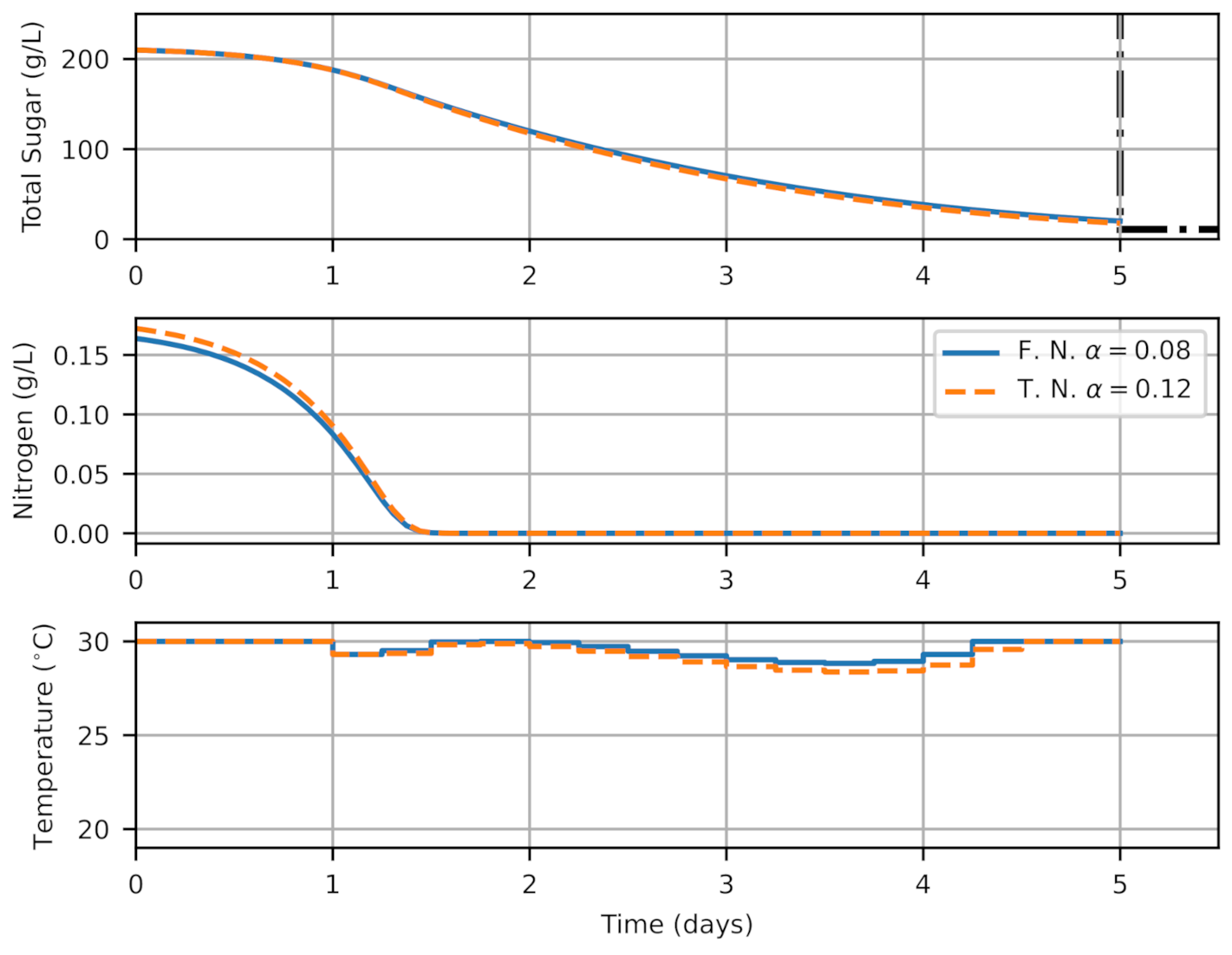
3.3. Comparison of the Most Suitable Strategies

Figure 6 shows the simulation of the optimal control solutions for FN and TN strategies on the knee point. Despite obtaining different Pareto fronts for FN and TN strategies (Figure 3 and Figure 5), the solutions on the knee point for both strategies were very similar. The nitrogen addition was concentrated only at the beginning of the fermentation, with DAP doses of 6.6 and 10.6 g/hL for FN and TN, respectively. Similarly, the sugar differences from the desired digging-out point were small: 9.16 and 6.7 g/L for FN and TN, respectively. Moreover, the fermentation temperature path was very similar for both strategies, characterized by high values (>27 °C) throughout the whole process. These strategies are ideal for red wine fermentations since high temperatures favor the extraction of phenolic compounds [2,3].
At the knee point, both strategies converge to similar solutions with DAP addition at the beginning of the fermentation. Nevertheless, an analysis of the Pareto fronts points in another direction. The TN has fewer degrees of freedom because it can only add nutrition at two opportunities. Because of this, it is more difficult to optimize the process, which leads to more scattered solutions and higher DAP use in most cases, as can be seen in Figure 5. In contrast, the FN has a smoother Pareto front and lower nitrogen use in most cases. These differences indicate that the FN strategy probably is more robust to changes in the parameters of the model or the objectives given by maceration time and final sugar content. The robustness of the strategies can be properly analyzed in future works.

4. Conclusions

An optimal control was developed to manage the digging-out point to improve the process efficiency and costs simultaneously. A trade-off between the minimization of the sugar concentration error at the digging-out point and the minimization of nitrogen additions using DAP was identified. Then, five MCDM algorithms were assessed to choose an optimal strategy from the Pareto front, using equal priorities for each objective. The selected solutions by MCDM were compared with the knee point. TOPSIS and LINMAP algorithms recommended identical solutions and coincided with the knee point for both free and traditional strategies.
Although the Pareto fronts were different for the FN and TN strategies, the solutions regarding the knee point were similar. The most suitable option was adding nitrogen only at the beginning of the fermentation (6.6–10.6 g/hL of DAP) and high fermentation temperatures (close to 30 °C), yielding the desired digging-out point with a small error (6–9 g/L). Thus, these strategies are a good option for red winemaking, favoring phenolic extraction. The methods described in this study can be extended to include quality indexes such as aroma production in white wines or phenolic extraction in red wines and can also be adapted to any fruit wine fermentation. Finally, it is planned for future work to integrate a phenolic extraction model with the fermentation model presented in this work. Thus, a multi-objective optimization problem will be formulated, including a quality index for the decision-making process.

Author Contributions

Conceptualization, R.L. and J.R.P.-C.; methodology, R.L. and B.M.L.; software, B.M.L.; validation, R.L. and J.R.P.-C.; formal analysis, R.L. and B.M.L.; investigation, R.L. and B.M.L.; data curation, B.M.L.; writing-original draft preparation, R.L.; writing-review and editing, B.M.L., J.E.N.-R., J.R.P.-C. and J.C.-V.; visualization, B.M.L.; supervision, R.L., J.C.-V., J.E.N.-R. and J.R.P.-C.; project administration, R.L.; funding acquisition, J.C.-V. All authors have read and agreed to the published version of the manuscript.

Funding

This research was funded by Corporación de Fomento de la Producción (CORFO), portfolio project 17PIDE-80701. J.E.N.R thanks CNPq under project 304032/2019-0.

Institutional Review Board Statement

Not applicable.

Informed Consent Statement

Not applicable.

Data Availability Statement

Not applicable.

Conflicts of Interest

The authors declare no conflict of interest.

Appendix A. Fermentation Model Equations

A simplified fermentation model of Zenteno et al. [9] presented in Torrealba et al. [22] is used here. The reduced Zenteno model is introduced as follows.
Differential equations:
Biomass generation and decay
d X d t = ( μ k d ) · X
Nitrogen consumption
d N d t = μ Y X N · X
Glucose consumption
d G d t = μ Y X G + β G Y E G + m · G G + F · X
Fructose consumption
d F d t = μ Y X F + β F Y E F + m · F G + F · X
Ethanol production
d E d t = ( β G + β F ) · X
Constitutive equations:
Specific growth rate
μ = μ m a x · N N + K N ( T )
Maximum growth rate
μ m a x = μ 0 · exp E a c · ( T 300 ) 300 · R · T
Biomass decay rate (when T> T d )
k d = k d 0 · exp ( C d e · E ) + E t d · T 305.65 305.65 · R · T
Thermal death ethanol-related threshold
T D = 0.0001 · E 3 + 0.0049 · E 2 0.1279 · E + 315.89
Ethanol production rate from fructose
β F = β F m a x · F F + K F ( T ) · K I G ( T ) G + K I G ( T ) · K I E ( T ) E + K I E ( T )
Ethanol production rate from glucose
β G = β G m a x · G G + K G ( T ) · K I E ( T ) E + K I E ( T )
Specific cell maintenance rate
m = m 0 · exp E a m · ( T 293.3 ) 293.3 · R · T
Maximum ethanol production rates
β i m a x = β i 0 · exp E a f e · ( T 296.15 ) 296.15 · R · T , i = G , F
Temperature inhibition parameters
K i ( T ) = K i 0 · exp E a k i · ( T T * ) 293.3 · R · T , i = N , G , F , i G , i E
The re-estimated parameter values are available in [22], and the rest of the parameters in [9].

References

  1. Cheynier, V.; Salas, E.; Souquet, J.M.; Sarni-manchado, P.; Fulcrand, H. Structure and Properties of Wine Pigments and Tannins. Am. J. Enol. Vitic. 2006, 57, 298–305. [Google Scholar]
  2. Setford, P.C.; Jeffery, D.W.; Grbin, P.R.; Muhlack, R.A. Modelling the Mass Transfer Process of Malvidin-3-Glucoside during Simulated Extraction from Fresh Grape Solids under Wine-Like Conditions. Molecules 2018, 23, 2159. [Google Scholar] [CrossRef] [PubMed] [Green Version]
  3. Setford, P.C.; Jeffery, D.W.; Grbin, P.R.; Muhlack, R.A. Factors affecting extraction and evolution of phenolic compounds during red wine maceration and the role of process modelling. Trends Food Sci. Technol. 2017, 69, 106–117. [Google Scholar] [CrossRef]
  4. Webb, L.B.; Whetton, P.H.; Barlow, E.W. Modelled impact of future climate change on the phenology of winegrapes in Australia. Aust. J. Grape Wine Res. 2007, 13, 165–175. [Google Scholar] [CrossRef]
  5. Luna, R.; Matias-Guiu, P.; López, F.; Pérez-Correa, J.R. Quality aroma improvement of Muscat wine spirits: A new approach using first-principles model-based design and multi-objective dynamic optimisation through multi-variable analysis techniques. Food Bioprod. Process. 2019, 115, 208–222. [Google Scholar] [CrossRef]
  6. Miller, K.V.; Block, D.E. A review of wine fermentation process modeling. J. Food Eng. 2020, 273, 109783. [Google Scholar] [CrossRef]
  7. Coleman, M.C.; Fish, R.; Block, D.E. Temperature-Dependent Kinetic Model for Nitrogen-Limited Wine Fermentations. Appl. Environ. Microbiol. 2007, 73, 5875–5884. [Google Scholar] [CrossRef] [PubMed] [Green Version]
  8. Cerda-Drago, T.G.; Agosin, E.; Pérez-Correa, J.R. Modelling the oxygen dissolution rate during oenological fermentation. Biochem. Eng. J. 2016, 106, 97–106. [Google Scholar] [CrossRef]
  9. Zenteno, M.I.; Pérez-Correa, J.R.; Gelmi, C.A.; Agosin, E. Modeling temperature gradients in wine fermentation tanks. J. Food Eng. 2010, 99, 40–48. [Google Scholar] [CrossRef]
  10. Miller, K.V.; Oberholster, A.; Block, D.E. Creation and validation of a reactor engineering model for multiphase red wine fermentations. Biotechnol. Bioeng. 2019, 116, 781–792. [Google Scholar] [CrossRef]
  11. Miller, K.V.; Noguera, R.; Beaver, J.; Oberholster, A.; Block, D.E. A combined phenolic extraction and fermentation reactor engineering model for multiphase red wine fermentation. Biotechnol. Bioeng. 2020, 117, 109–116. [Google Scholar] [CrossRef]
  12. Ashoori, A.; Moshiri, B.; Khaki-Sedigh, A.; Bakhtiari, M.R. Optimal control of a nonlinear fed-batch fermentation process using model predictive approach. J. Process Control 2009, 19, 1162–1173. [Google Scholar] [CrossRef]
  13. Santos, L.; Dewasme, L.; Coutinho, D.; Wouwer, A.V. Nonlinear model predictive control of fed-batch cultures of micro-organisms exhibiting overflow metabolism: Assessment and robustness. Comput. Chem. Eng. 2012, 39, 143–151. [Google Scholar] [CrossRef]
  14. Craven, S.; Whelan, J.; Glennon, B. Glucose concentration control of a fed-batch mammalian cell bioprocess using a nonlinear model predictive controller. J. Process Control 2014, 24, 344–357. [Google Scholar] [CrossRef]
  15. Chang, L.; Liu, X.; Henson, M.A. Nonlinear model predictive control of fed-batch fermentations using dynamic flux balance models. J. Process Control 2016, 42, 137–149. [Google Scholar] [CrossRef]
  16. Schenk, C.; Schulz, V.; Rosch, A.; von Wallbrunn, C. Less cooling energy in wine fermentation—A case study in mathematical modeling, simulation and optimization. Food Bioprod. Process. 2017, 103, 131–138. [Google Scholar] [CrossRef]
  17. Vaccari, M.; Bacci di Capaci, R.; Brunazzi, E.; Tognotti, L.; Pierno, P.; Vagheggi, R.; Pannocchia, G. Optimally Managing Chemical Plant Operations: An Example Oriented by Industry 4.0 Paradigms. Ind. Eng. Chem. Res. 2021. [Google Scholar] [CrossRef]
  18. Narayanan, H.; Luna, M.F.; von Stosch, M.; Cruz Bournazou, M.N.; Polotti, G.; Morbidelli, M.; Butté, A.; Sokolov, M. Bioprocessing in the Digital Age: The Role of Process Models. Biotechnol. J. 2020, 15, 1900172. [Google Scholar] [CrossRef]
  19. The Association for Packaging and Processing Technologies, Inc. How to Utilize Big Data to Enhance Manufacturing Processes; Technical Report; The Association for Packaging and Processing Technologies, Inc.: Herndon, VA, USA, 2018. [Google Scholar]
  20. Rodman, A.D.; Gerogiorgis, D.I. Multi-objective process optimisation of beer fermentation via dynamic simulation. Food Bioprod. Process. 2016, 100, 255–274. [Google Scholar] [CrossRef] [Green Version]
  21. Luna, R.; López, F.; Pérez-Correa, J.R. Design of optimal wine distillation recipes using multi-criteria decision-making techniques. Comput. Chem. Eng. 2021, 145, 107194. [Google Scholar] [CrossRef]
  22. Torrealba, C.; Luna, R.; Cuevas-Valenzuela, J.; Pérez-Correa, J.R. A multi-criteria decision making guided parametric robustness assessment workflow: Enhancing wine fermentation models in the presence of limited data structures. 2021, submitted.
  23. Casassa, L.F.; Larsen, R.C.; Beaver, C.W.; Mireles, M.S.; Keller, M.; Riley, W.R.; Smithyman, R.; Harbertson, J.F. Impact of Extended Maceration and Regulated Deficit Irrigation (RDI) in Cabernet Sauvignon Wines: Characterization of Proanthocyanidin Distribution, Anthocyanin Extraction, and Chromatic Properties. J. Agric. Food Chem. 2013, 61, 6446–6457. [Google Scholar] [CrossRef]
  24. Bhaskar, V.; Gupta, S.K.; Ray, A.K. Applications of multiobjective optimization in chemical engineering. Rev. Chem. Eng. 2000, 16, 1–54. [Google Scholar] [CrossRef]
  25. Miettinen, K.; Hakanen, J. Why Use Interactive Multi-Objective Optimization in Chemical Process Design. In MULTI-OBJECTIVE OPTIMIZATION: Techniques and Application in Chemical Engineering; World Scientific: Singapore, 2008; pp. 153–188. [Google Scholar] [CrossRef] [Green Version]
  26. Ministerio de Agricultura, Biblioteca del Congreso Nacional de Chile. Reglamenta Ley N° 18455 que fija normas sobre producción, elaboración y comercialización de alcoholes etilicos, bebidas alcoholicas y vinagres. 1986. Available online: https://www.bcn.cl/leychile/navegar?idNorma=8815 (accessed on 3 June 2021).
  27. Kameswaran, S.; Biegler, L.T. Simultaneous dynamic optimization strategies: Recent advances and challenges. Comput. Chem. Eng. 2006, 30, 1560–1575. [Google Scholar] [CrossRef]
  28. Biegler, L.T. 10. Simultaneous Methods for Dynamic Optimization. In Nonlinear Programming; SIAM: Philadelphia, PA, USA, 2010; Chapter 10; pp. 287–324. [Google Scholar] [CrossRef]
  29. Biegler, L.T. An overview of simultaneous strategies for dynamic optimization. Chem. Eng. Process. Process Intensif. 2007, 46, 1043–1053. [Google Scholar] [CrossRef]
  30. Andersson, J.A.E.; Gillis, J.; Horn, G.; Rawlings, J.B.; Diehl, M. CasADi—A software framework for nonlinear optimization and optimal control. Math. Program. Comput. 2019, 11, 1–36. [Google Scholar] [CrossRef]
  31. Wächter, A.; Biegler, L. On the implementation of an interior-point filter line-search algorithm for large-scale nonlinear programming. Math. Program. 2006, 106, 25–57. [Google Scholar] [CrossRef]
  32. Pérez, D.; Assof, M.; Bolcato, E.; Sari, S.; Fanzone, M. Combined effect of temperature and ammonium addition on fermentation profile and volatile aroma composition of Torrontés Riojano wines. LWT 2018, 87, 488–497. [Google Scholar] [CrossRef]
  33. Mouret, J.; Farines, V.; Sablayrolles, J.; Trelea, I. Prediction of the production kinetics of the main fermentative aromas in winemaking fermentations. Biochem. Eng. J. 2015, 103, 211–218. [Google Scholar] [CrossRef]
  34. Wang, Z.; Rangaiah, G.P. Application and Analysis of Methods for Selecting an Optimal Solution from the Pareto-Optimal Front obtained by Multiobjective Optimization. Ind. Eng. Chem. Res. 2017, 56, 560–574. [Google Scholar] [CrossRef]
  35. Chiu, W.Y.; Yen, G.G.; Juan, T.K. Minimum Manhattan Distance Approach to Multiple Criteria Decision Making in Multiobjective Optimization Problems. IEEE Trans. Evol. Comput. 2016, 20, 972–985. [Google Scholar] [CrossRef] [Green Version]
  36. Branke, J.; Deb, K.; Dierolf, H.; Osswald, M. Finding Knees in Multi-objective Optimization. In Parallel Problem Solving from Nature—PPSN VIII; Yao, X., Burke, E.K., Lozano, J.A., Smith, J., Merelo-Guervós, J.J., Bullinaria, J.A., Rowe, J.E., Tiňo, P., Kabán, A., Schwefel, H.P., Eds.; Springer: Berlin/Heidelberg, Germany, 2004; pp. 722–731. [Google Scholar]
  37. Weise, T. Global Optimization Algorithms—Theory and Application. 2nd ed.; Self-Published. 2009. Available online: http://www.it-weise.de/ (accessed on 2 June 2021).
Figure 1. Scheme for industrial bulk red winemaking: fermentative maceration (1) and alcoholic fermentation completion (2). The blue line represents the juice fed at the digging-out point to complete the alcoholic fermentation, and the green line represents the solids (pomace) fed to produce press wines.
Fermentation 07 00094 g001
Figure 2. Optimal control simulations for free nutrition strategies. Black line in total sugar graph corresponds to the desired digging-out point.
Fermentation 07 00094 g002
Figure 3. Pareto front for free nutrition strategies, optimal solutions selected by MCDM algorithms and knee point. Points corresponding to α = 0 and α = 1 are omitted.
Fermentation 07 00094 g003
Figure 4. Optimal control simulations for traditional nutrition. Black line in total sugar graph corresponds to the desired digging-out point.
Fermentation 07 00094 g004
Figure 5. Pareto front with DAP addition at t = 0 h and t = 48 h. Total of 50 points with 0.05 step. The points corresponding to α = 0 and α = 1 are omitted.
Fermentation 07 00094 g005
Figure 6. Comparison of the chosen optimal control strategies. Black line in total sugar graph corresponds to the desired digging-out point.
Fermentation 07 00094 g006
Table 1. Initial conditions for state variables.
State VariablesNomenclatureValues
Biomass X ( 0 ) 0.200 g/L
Nitrogen N ( 0 ) 0.150 g/L
Glucose G ( 0 ) 105 g/L
Fructose F ( 0 ) 105 g/L
Ethanol E ( 0 ) 0 g/L
Publisher’s Note: MDPI stays neutral with regard to jurisdictional claims in published maps and institutional affiliations.

