
Hexagonal-Shaped Spin Crossover Nanoparticles Studied by Ising-Like Model Solved by Local Mean Field Approximation

 , , and
Abstract
:1. Introduction
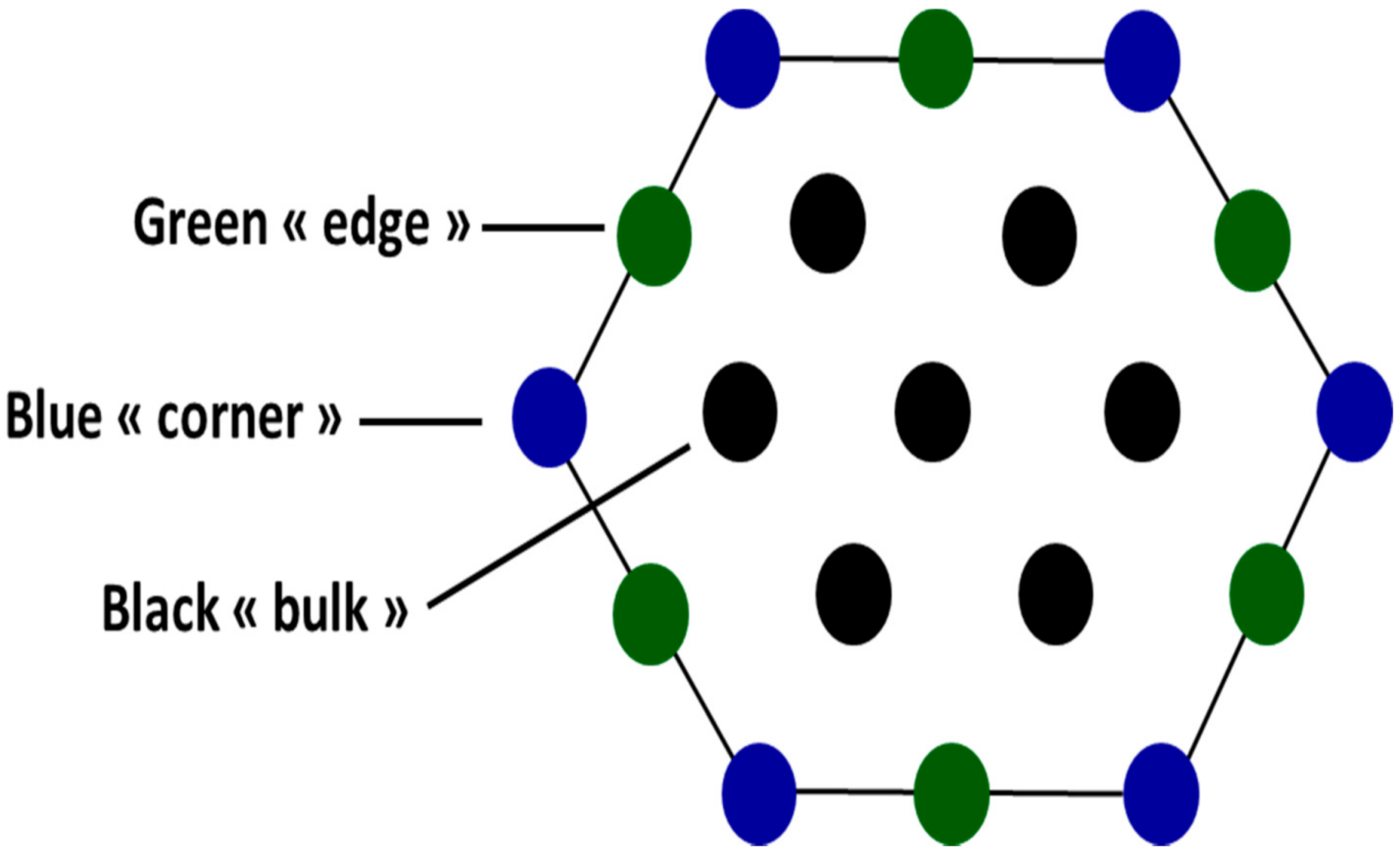
2. Model
3. Numerical Results and Discussion
3.1. Case L = 0
3.2. Case L ≠ 0
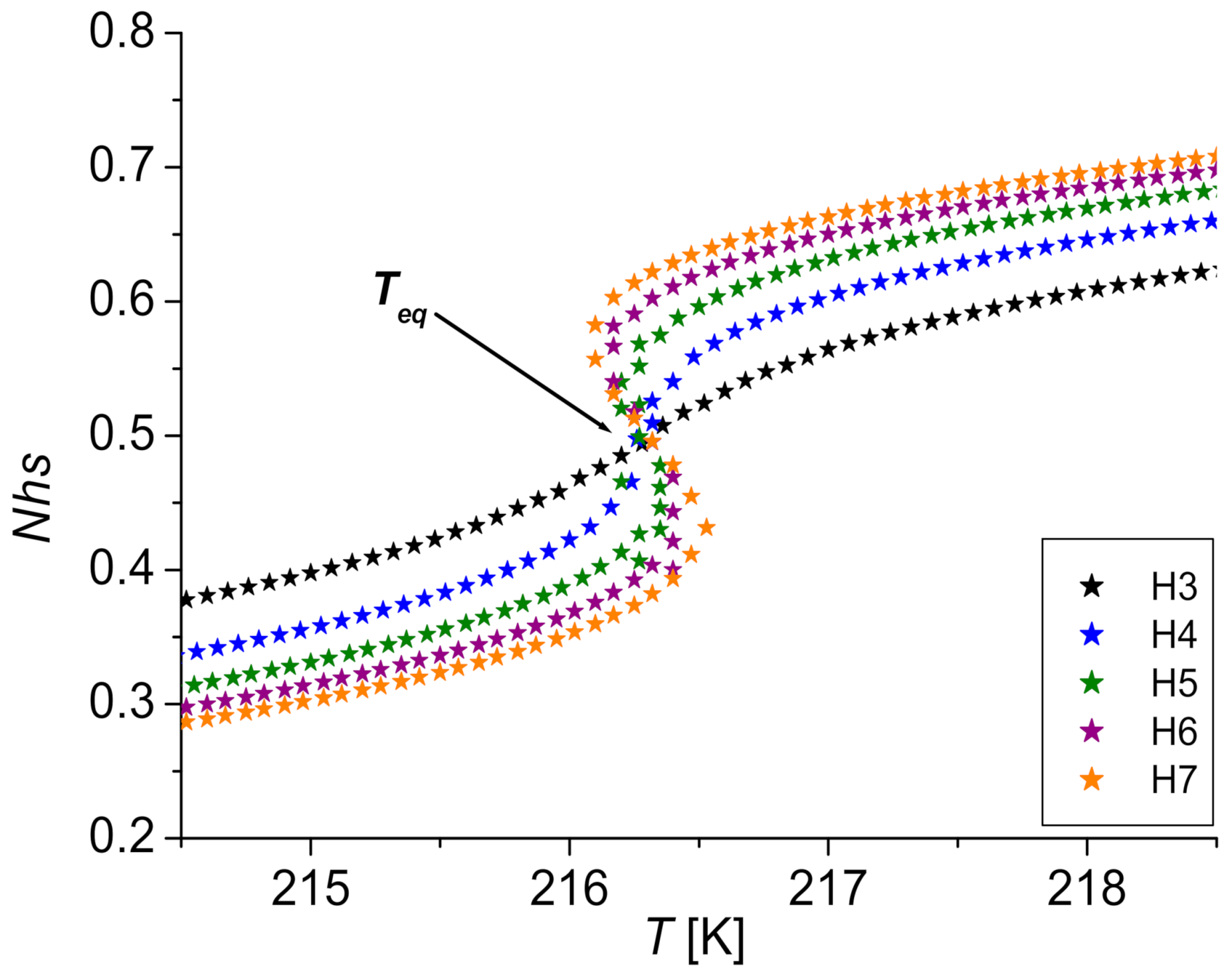
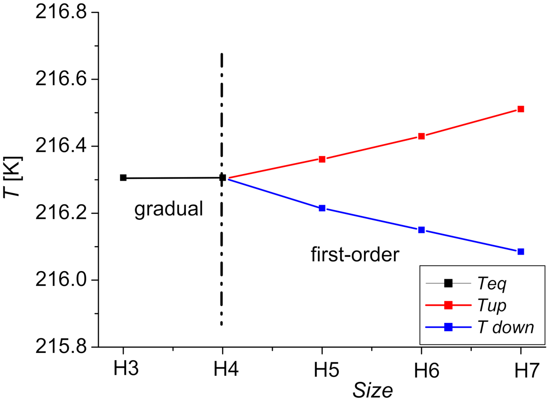
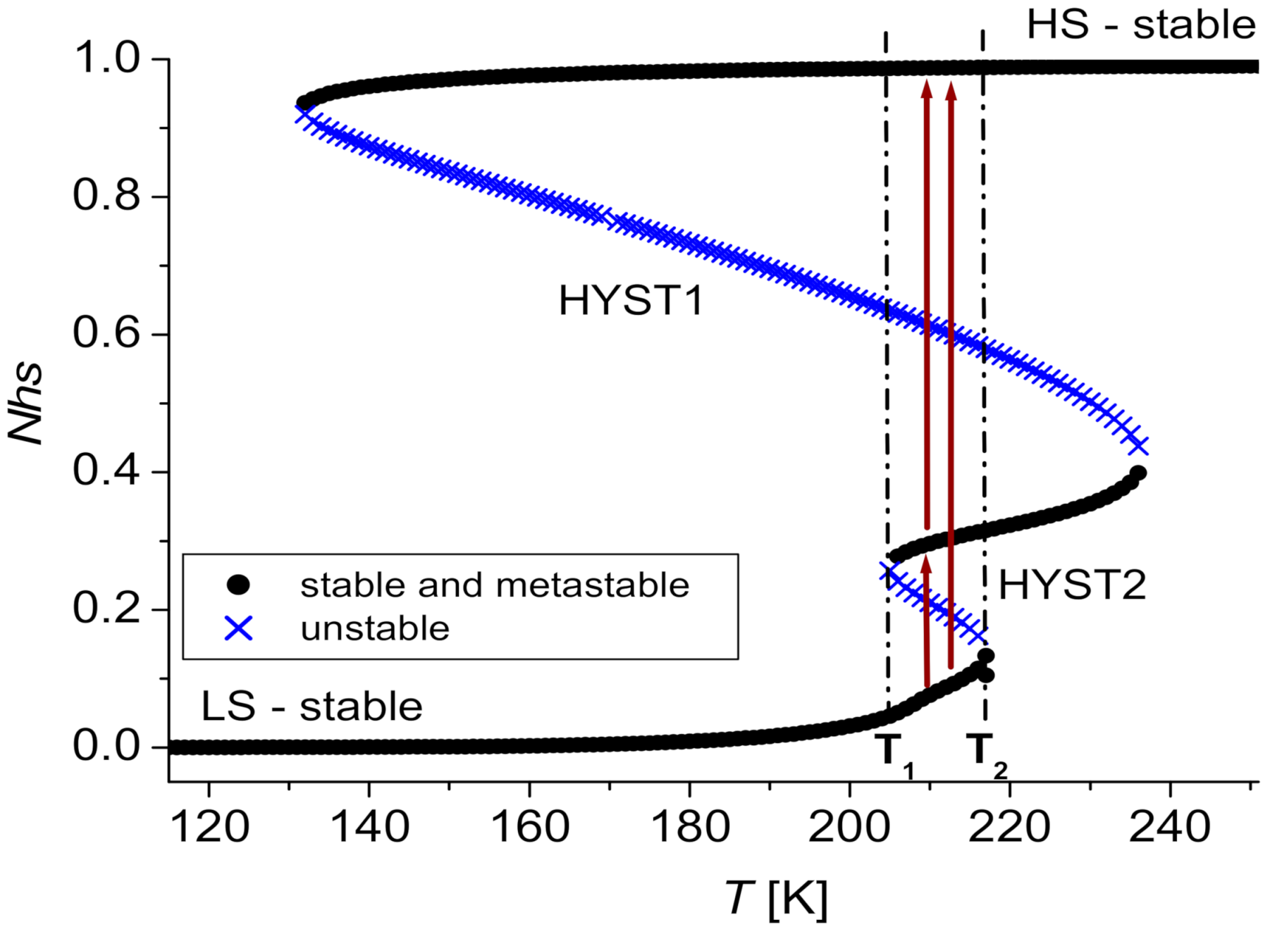
3.2.1. Three Steps
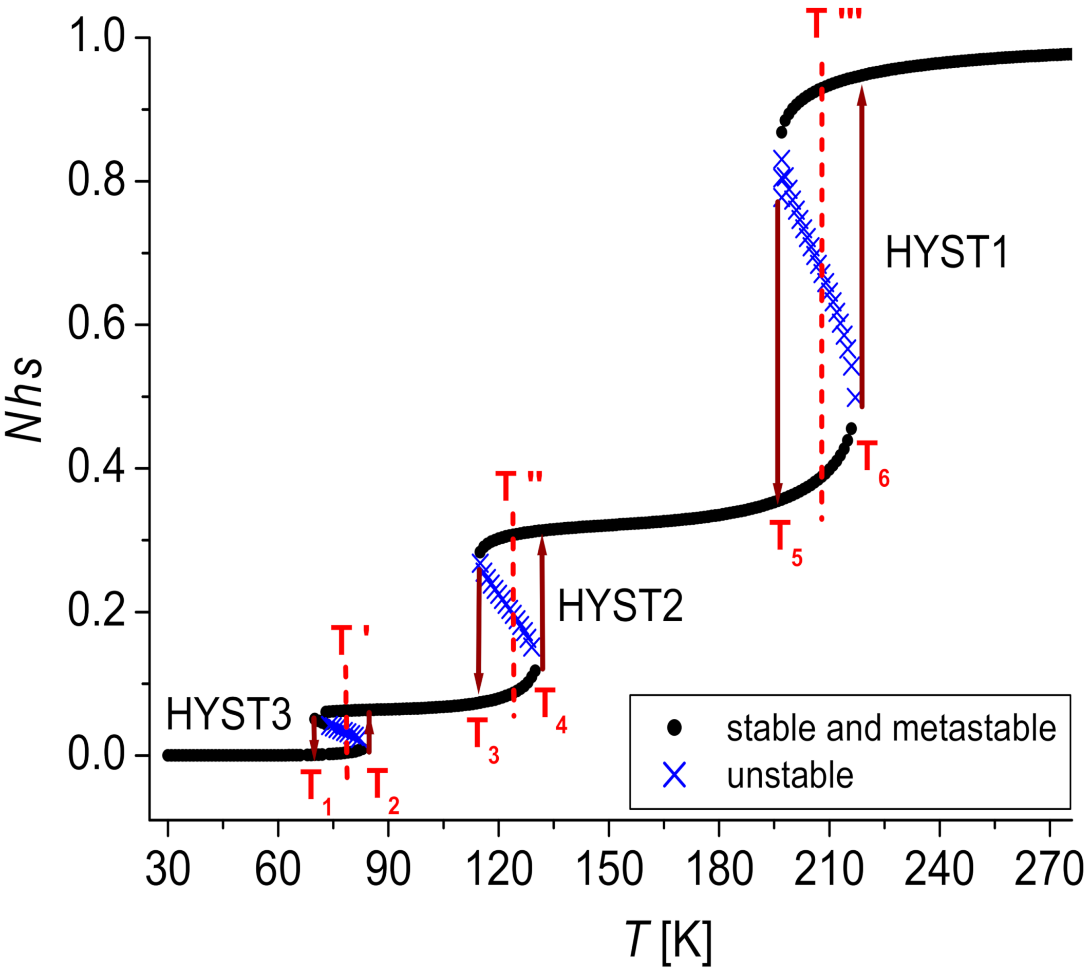
3.2.2. Three States
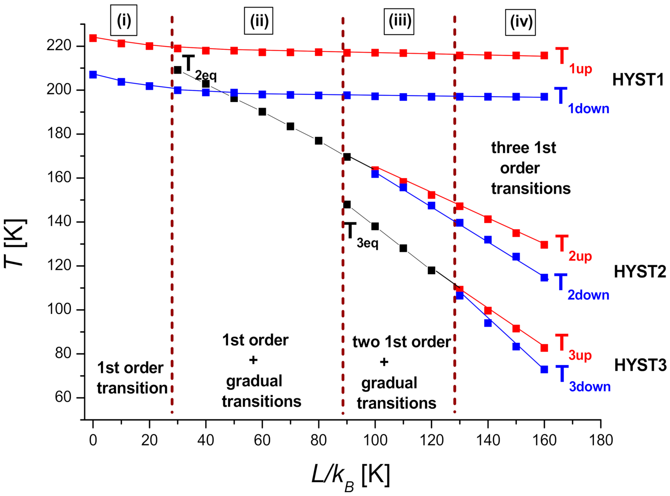
4. Phase Diagram
5. Conclusions
Author Contributions
Funding
Data Availability Statement
Acknowledgments
Conflicts of Interest
References
- Tour, J.M. Introduction to Molecular Electronics. J. Am. Chem. Soc. 1996, 118, 2309–2310. [Google Scholar] [CrossRef]
- Gutlich, P. Spin crossover in iron(II)-complexes. In Metal Complexes; Structure and Bonding; Springer: Berlin/Heidelberg, Germany, 1981; Volume 44, pp. 83–195. [Google Scholar] [CrossRef]
- Molnar, G.; Niel, V.; Real, J.A.; Dubrovinsky, L.; Bousseksou, A.; McGarvey, J.J. Raman Spectroscopic Study of Pressure Effects on the Spin-Crossover Coordination Polymers Fe(Pyrazine)[M(CN)4]·2H2O (M = Ni, Pd, Pt). First Observation of a Piezo-Hysteresis Loop at Room Temperature. J. Phys. Chem. B 2003, 107, 3149–3155. [Google Scholar] [CrossRef]
- Krober, J.; Audière, J.P.; Claude, R.; Kahn, O.; Hassnoot, J.; Grolière, F.; Jay, C.; Bousseksou, A.; Linares, J.; Varret, F.; et al. Spin Transitions and Thermal Hysteresis in the Molecular-Based Materials [Fe(Htrz)2(trz)](BF4) and [Fe(Htrz)3](BF4)2.cntdot.H2O (Htrz = 1,2,4-4H-triazole; trz = 1,2,4-triazolato). Chem. Mater. 1994, 6, 1404–1412. [Google Scholar] [CrossRef]
- Roubeau, O.; Stassen, A.F.; Ferrero-Gramage, I.; Codjovi, E.; Linares, J.; Varret, F.; Haasnoot, J.G.; Reedjik, J. Surprising features in old and new [Fe(alkyl-tetrazole)6] spin-crossover systems. Polyhedron 2001, 20, 1709–1716. [Google Scholar] [CrossRef]
- Clements, J.E.; Price, J.R.; Neville, S.M.; Kepert, C.J. Hysteretic Four-Step Spin Crossover within a Three-Dimensional Porous Hofmann-like Material. Angew. Chem. Int. Ed. 2016, 55, 15105–15109. [Google Scholar] [CrossRef]
- Dirtu, M.M.; Garcia, Y.; Nica, M.; Rotaru, A.; Linares, J.; Varret, F. Iron(II) spin transition 1,2,4-triazole chain compounds with novel inorganic fluorinated counteranions. Polyhedron 2007, 26, 2259–2263. [Google Scholar] [CrossRef]
- Boca, R.; Salitros, I.; Kozisek, J.; Linares, J.; Moncol, J.; Renz, F. Spin crossover in a heptanuclear mixed-valence iron complex. Dalton Trans. 2010, 39, 2198–2200. [Google Scholar] [CrossRef]
- Constant-Machado, H.; Stancu, A.; Linares, J.; Varret, F. Thermal hysteresis loops in spin-crossover compounds analyzed in terms of classical Preisach model. IEEE Trans. Magn. 1998, 34, 2213–2219. [Google Scholar] [CrossRef]
- Boukheddaden, K.; Ritti, M.H.; Bouchez, G.; Sy, M.; Dirtu, M.M.; Parlier, P.; Linares, J.; Garcia, Y. Quantitative Contact Pressure Sensor Based on Spin Crossover Mechanism for Civil Security Applications. J. Phys. Chem. C 2018, 122, 7597–7604. [Google Scholar] [CrossRef]
- Jeftic, J.; Hauser, A. Pressure Study of the Thermal Spin Transition and the High-Spin → Low-Spin Relaxation in the R3− and P1− Crystallographic Phases of [Zn1-xFex(ptz)6](BF4)2 Single Crystals (x = 0.1, 0.32, and 1; ptz = 1-n-propyltetrazole). J. Phys. Chem. B 1997, 101, 10262–10270. [Google Scholar] [CrossRef]
- Rotaru, A.; Linares, J.; Varret, F.; Codjovi, E.; Slimani, A.; Tanasa, R.; Enachescu, C.; Stancu, A.; Haasnoot, J. Pressure effect investigated with first-order reversal-curve method on the spin-transition compounds [FexZn1−x(btr)2(NCS)2] ⋅ H2O (x=0.6,1). Phys. Rev. B 2011, 83, 224107–224114. [Google Scholar] [CrossRef]
- Decurtins, S.; Gutlich, P.; Kohler, C.P.; Spiering, H.; Hauser, A. Light-induced excited spin state trapping in a transition-metal complex: The hexa-1-propyltetrazole-iron (II) tetrafluoroborate spin-crossover system. Chem. Phys. Lett. 1984, 105, 1–4. [Google Scholar] [CrossRef]
- Gütlich, P.; Hauser, A.; Spiering, H. Thermal and Optical Switching of Iron(II) Complexes. Angew. Chem. Int. Edit. 1994, 33, 2024–2054. [Google Scholar] [CrossRef]
- Bonhommeau, S.; Molnar, G.; Galet, A.; Zwick, A.; Real, J.A.; McGarvey, J.F.; Bousseksou, A. One Shot Laser Pulse Induced Reversible Spin Transition in the Spin-Crossover Complex [Fe(C4H4N2){Pt(CN)4}] at Room Temperature. Angew. Chem. Int. Ed. 2005, 44, 4069–4073. [Google Scholar] [CrossRef]
- Moussa, N.O.; Molnar, G.; Bonhommeau, S.; Zwick, A.; Mouri, S.; Tanaka, K.; Real, J.A.; Bousseksou, A. Selective Photoswitching of the Binuclear Spin Crossover Compound {[Fe(bt)(NCS)2]2(bpm)} into Two Distinct Macroscopic Phases. Phys. Rev. Lett. 2005, 94, 107205–107208. [Google Scholar] [CrossRef]
- Decurtins, S.; Gutlich, P.; Hasselbach, K.M.; Hauser, A.; Spiering, H. Light-induced excited-spin-state trapping in iron(II) spin-crossover systems. Optical spectroscopic and magnetic susceptibility study. Inorg. Chem. 1985, 24, 2174–2178. [Google Scholar] [CrossRef]
- Enachescu, C.; Menendez, N.; Codjovi, E.; Linares, J.; Varret, F.; Stancu, A. Static and light induced hysteresis in spin-crossover compounds: Experimental data and application of Preisach-type models. Physica B Condens. Matter 2001, 306, 155–160. [Google Scholar] [CrossRef]
- Bousseksou, A.; Boukheddaden, K.; Goiran, M.; Consejo, C.; Boillot, M.L.; Tuchagues, J.P. Dynamic response of the spin-crossover solid Co(H2(fsa)2en)(py)2 to a pulsed magnetic field. Phys. Rev. B 2002, 65, 172412–172415. [Google Scholar] [CrossRef]
- Chastanet, G.; Gaspar, A.B.; Real, J.A.; Letard, J.-F. Photo-switching spin pairs-synergy between LIESST effect and magnetic interaction in an iron(II) binuclear spin-crossover compound. Chem. Commun. 2001, 9, 819–820. [Google Scholar] [CrossRef] [Green Version]
- Maddock, A.G.; Schleiffer, J. Spin cross-over and the Mössbauer emission spectrum of cobalt-57-labelled di-isothiocyanatobis(1,10-phenanthroline)-iron(II) and -cobalt(II). J. Chem. Soc. Dalton Trans. 1977, 7, 617–620. [Google Scholar] [CrossRef]
- Sy, M.; Varret, F.; Boukheddaden, K.; Bouchez, G.; Marrot, J.; Kawata, S.; Kaizaki, S. Structure-Driven Orientation of the High-Spin–Low-Spin Interface in a Spin-Crossover Single Crystal. Angew. Chem. Int. Ed. 2014, 53, 7539–7542. [Google Scholar] [CrossRef] [PubMed]
- Shepherd, H.J.; Bonnet, S.; Guionneau, P.; Bedoui, S.; Garbarino, G.; Nicolazzi, W.; Bousseksou, A.; Molnár, G. Pressure-induced two-step spin transition with structural symmetry breaking: X-ray diffraction, magnetic, and Raman studies. Phys. Rev. B 2011, 84, 144107–144115. [Google Scholar] [CrossRef] [Green Version]
- Castro, M.; Rodríguez-Velamazaán, J.A.; Boukheddaden, K.; Varret, F.; Tokoro, H.; Ohkoshi, S. Calorimetric investigation of equilibrium and thermal relaxation properties of the switchable Prussian Blue analog Na0.32Co[Fe(CN)6]0.74.3.4H2O. Eur. Phys. Lett. 2007, 79, 27007–27012. [Google Scholar] [CrossRef]
- Toftlund, H. Spin equilibria in iron(II) complexes. Coord. Chem. Rev. 1989, 94, 67–108. [Google Scholar] [CrossRef]
- König, E. Some aspects of the chemistry of bis(2,2′-dipyridyl) and bis(1,10-phenanthroline) complexes of iron(II). Coord. Chem. Rev. 1968, 3, 471–495. [Google Scholar] [CrossRef]
- Oyanagi, H.; Tayagaki, T.; Tanaka, K. Synchrotron radiation study of photo-induced spin-crossover transitions: Microscopic origin of nonlinear phase transition. J. Lumin. 2006, 361, 119–120. [Google Scholar] [CrossRef]
- König, E.; Ritter, G. Hysteresis effects at a cooperative high-spin (5T2) ⇌ low-spin (1A1) transition in dithiocyanatobis (4, 7-dimethyl-1, 10-phenanthroline) iron (II). Solid State Commun. 1976, 18, 279–282. [Google Scholar] [CrossRef]
- Zelentsov, V.V. Spin transitions in iron (III) complexes with thiosemicarbazones of O-hydroxyaldehydes. Sov. Sci. Rev. B Chem. 1987, 10, 485–512. [Google Scholar]
- Sciortino, N.F.; Scherl-Gruenwald, K.R.; Chastanet, G.; Halder, G.J.; Chapman, K.W.; Letard, J.-F.; Kepert, C.J. Hysteretic three-step spin crossover in a thermo- and photochromic 3D pillared Hofmann-type metal-organic framework. Angew. Chem. Int. Ed. 2012, 51, 10154–10158. [Google Scholar] [CrossRef]
- Kosone, T.; Tomori, I.; Kanadani, C.; Saito, T.; Mochida, T.; Kitazawa, T. Unprecedented three-step spin-crossover transition in new 2-dimensional coordination polymer{FeII(4-methylpyridine)2[AuI(CN)2]2}. Dalton Trans. 2010, 39, 1719–1721. [Google Scholar] [CrossRef]
- Nishi, K.; Kondo, H.; Fujinami, T.; Matsumoto, N.; Iijima, S.; Halcrow, M.A.; Sunatsuki, Y.; Kojima, M. Stepwise Spin Transition and Hysteresis of Tetrameric Iron(II) Complex, fac-[Tris(2-methylimidazol-4-ylmethylidene-n-hexylamine)]iron(II)Chloride Hexafluorophosphate, Assembled by Imidazole…Chloride Hydrogen Bonds. Eur. J. Inorg. Chem. 2013, 5/6, 927–933. [Google Scholar] [CrossRef]
- Wajnflasz, J.; Pick, R. Transitions «low spin»-«high spin» dans les complexes de Fe2+. J. Phys. Colloq. 1971, 32, 91–92. [Google Scholar] [CrossRef]
- Bousseksou, A.; Nasser, J.; Linares, J.; Boukheddaden, K.; Varret, F. Ising-like model for the two-step spin-crossover. J. Phys. I Fr. 1992, 2, 1381–1403. [Google Scholar] [CrossRef]
- Linares, J.; Jureschi, C.; Boukheddaden, K. Surface Effects Leading to Unusual Size Dependence of the Thermal Hysteresis Behavior in Spin-Crossover Nanoparticles. Magnetochemistry 2016, 2, 24. [Google Scholar] [CrossRef] [Green Version]
- Linares, J.; Jureschi, C.; Boulmaali, A.; Boukheddaden, K. Matrix and size effects on the appearance of the thermal hysteresis in 2D spin crossover nanoparticles. Phys. B Condens. Matter 2016, 486, 164–168. [Google Scholar] [CrossRef]
- Nasser, J.A.; Boukheddaden, K.; Linares, J. Two-step spin conversion and other effects in the atom-phonon coupling model. Eur. Phys. J. B 2004, 39, 219–227. [Google Scholar] [CrossRef]
- Enachescu, C.; Nishino, M.; Miyashita, S.; Hauser, A.; Stancu, A.; Stoleriu, L. Cluster evolution in spin crossover systems observed in the frame of a mechano-elastic model. Eur. Phys. Lett. 2010, 91, 27003. [Google Scholar] [CrossRef]
- Slimani, A.; Boukheddaden, K.; Varret, F.; Oubouchou, H.; Nishino, M.; Miyashita, S. Microscopic spin-distortion model for switchable molecular solids: Spatiotemporal study of the deformation field and local stress at the thermal spin transition. Phys. Rev. B 2013, 87, 014111–014120. [Google Scholar] [CrossRef]
- Linares, J.; Spiering, H.; Varret, F. Analytical solution of 1D Ising-like systems modified by weak long range interaction. Eur. Phys. J. B 1999, 10, 271–275. [Google Scholar] [CrossRef]
- Chiruta, D.; Jureschi, C.M.; Linares, J.; Dahoo, P.R.; Garcia, Y.; Rotaru, A. On the origin of multi-step spin transition behaviour in 1D nanoparticles. Eur. Phys. J. B 2015, 88, 233–237. [Google Scholar] [CrossRef]
- Allal, S.E.; Harlé, C.; Sohier, D.; Dufaud, T.; Dahoo, P.R.; Linares, J. Three Stable States Simulated for 1D Spin-Crossover Nanoparticles Using the Ising-Like Model. Eur. J. Inorg. Chem. 2017, 4196–4201. [Google Scholar] [CrossRef]
- Allal, S.E.; Linares, J.; Boukheddaden, K.; Dahoo, P.R.; de Zela, F. 2D Spin Crossover Nanoparticles described by the Ising-like model solved in Local Mean-Field Approximation. J. Phys. Conf. Ser. 2017, 936, 012052–012058. [Google Scholar] [CrossRef]
- Allal, S.E.; Sohier, D.; Dufaud, T.; Harlé, C.; Dahoo, P.R.; Linares, J. Size effect on the three state thermal hysteresis of a 2D spin crossover nanoparticles. J. Phys. Conf. Ser. 2018, 1141, 012158–012174. [Google Scholar] [CrossRef]
- Cazelles, C.; Singh, Y.; Linares, J.; Dahoo, P.R.; Boukheddaden, K. Three states and three steps simulated within Ising like model solved by local mean field approximation in 3D spin crossover nanoparticles. Mater. Today Commun. 2021, 26, 102074–102083. [Google Scholar] [CrossRef]
- Chiruta, D.; Linares, J.; Garcia, Y.; Dimian, M.; Dahoo, P.R. Analysis of multi-step transitions in spin crossover nanochains. Phys. B Condens. Matter 2014, 434, 134–138. [Google Scholar] [CrossRef]
- Chiruta, D.; Linares, J.; Dahoo, P.R.; Dimian, M. Influence of pressure and interactions strength on hysteretic behavior in two-dimensional polymeric spin crossover compounds. Phys. B Condens. Matter 2014, 435, 76–79. [Google Scholar] [CrossRef]
- Muraoka, A.; Boukheddaden, K.; Linares, J.; Varret, F. Two-dimensional Ising-like model with specific edge effects for spin-crossover nanoparticles: A Monte Carlo study. Phys. Rev. B 2011, 84, 054119–054125. [Google Scholar] [CrossRef]


| Site | Bulk | Edge | Corner |
|---|---|---|---|
| ligand-field |
| Size of the System | Ns = Nc + Ne | NT | r = Ns/NT |
|---|---|---|---|
| H3 | 12 | 19 | 0.63 |
| H4 | 18 | 37 | 0.48 |
| H5 | 24 | 61 | 0.39 |
| H6 | 30 | 91 | 0.32 |
| H7 | 36 | 127 | 0.28 |
| 0 | 216.30 | 216.30 | 216.30 | 216.30 |
| 50 | 166.38 | 183.02 | 216.30 | 204.23 |
| 120 | 96.50 | 136.43 | 216.30 | 187.33 |
| 160 | 56.57 | 109.81 | 216.30 | 177.68 |
Publisher’s Note: MDPI stays neutral with regard to jurisdictional claims in published maps and institutional affiliations. |
© 2021 by the authors. Licensee MDPI, Basel, Switzerland. This article is an open access article distributed under the terms and conditions of the Creative Commons Attribution (CC BY) license (https://creativecommons.org/licenses/by/4.0/).
Share and Cite
Cazelles, C.; Linares, J.; Ndiaye, M.; Dahoo, P.-R.; Boukheddaden, K. Hexagonal-Shaped Spin Crossover Nanoparticles Studied by Ising-Like Model Solved by Local Mean Field Approximation. Magnetochemistry 2021, 7, 69. https://0-doi-org.brum.beds.ac.uk/10.3390/magnetochemistry7050069
Cazelles C, Linares J, Ndiaye M, Dahoo P-R, Boukheddaden K. Hexagonal-Shaped Spin Crossover Nanoparticles Studied by Ising-Like Model Solved by Local Mean Field Approximation. Magnetochemistry. 2021; 7(5):69. https://0-doi-org.brum.beds.ac.uk/10.3390/magnetochemistry7050069
Chicago/Turabian StyleCazelles, Catherine, Jorge Linares, Mamadou Ndiaye, Pierre-Richard Dahoo, and Kamel Boukheddaden. 2021. "Hexagonal-Shaped Spin Crossover Nanoparticles Studied by Ising-Like Model Solved by Local Mean Field Approximation" Magnetochemistry 7, no. 5: 69. https://0-doi-org.brum.beds.ac.uk/10.3390/magnetochemistry7050069