Pulse Reverse Plating of Copper Micro-Structures in Magnetic Gradient Fields

Abstract

Micro-structured copper layers are obtained from pulse-reverse electrodeposition on a planar gold electrode that is magnetically patterned by magnetized iron wires underneath. 3D numerical simulations of the electrodeposition based on an adapted reaction kinetics are able to nicely reproduce the micro-structure of the deposit layer, despite the height values still remain underestimated. It is shown that the structuring is enabled by the magnetic gradient force, which generates a local flow that supports deposition and hinders dissolution in the regions of high magnetic gradients. The Lorentz force originating from radial magnetic field components near the rim of the electrode causes a circumferential cell flow. The resulting secondary flow, however, is superseded by the local flow driven by the magnetic gradient force in the vicinity of the wires. Finally, the role of solutal buoyancy effects is discussed to better understand the limitations of structured growth in different modes of deposition and cell geometries.

1. Introduction

Structured metal layers are of high interest in fields including microelectronics, microcopies and electrocatalysis [1,2]. Among the various methods of fabricating metal layers, electrodeposition is a well-established approach for mass production. However, expensive masking or template techniques are often required to obtain layers with micro-structures [3,4].

In order to simplify the manufacturing process, a mask-free method has been developed in the last decade, where structured deposit layers grow from planar but magnetically patterned electrodes. The method has been used to grow dendritic Ni structures by using a magnetized steel mesh [5], dot or antidot micro-structures of Cu and Zn by using arrays of NdFeB magnets [6,7] and micro-structured layers of Cu, Co, Fe and CoFe alloys by using arrays of magnetized iron wires [8,9,10]. Besides, also reversely structured metal layers from diamagnetic metal ions (e.g., Bi${}^{3+}$) may be grown when electrochemically inert paramagnetic ions (e.g., Mn${}^{2+}$) are added to the electrolyte [11,12]. In all cases, the magnetic patterning causes locally inhomogeneous magnetic fields in the vicinity of the electrode which allow to obtain structured deposits in the μm scale. The structured growth observed was found to be caused by the magnetic gradient force, defined as [13]:

$${\mathit{f}}_{\nabla \mathrm{B}}={\chi }_{\mathrm{sol}}/{\mu }_0(\mathit{B}·\nabla )\mathit{B},{\chi }_{\mathrm{sol}}=\sum _i{\chi }_i^{\mathrm{mol}}{c}_i+{\chi }_{{\mathrm{H}}_2\mathrm{O}},$$

(1)

with ${\mu }_0,\mathit{B},c_i,{\chi }_i^{\mathrm{mol}},{\chi }_{\mathrm{sol}},{\chi }_{{\mathrm{H}}_2\mathrm{O}}$ representing the vacuum permeability, the magnetic flux density, the concentration and the molar magnetic susceptibility of species i, the magnetic susceptibility of the solution and water, respectively. During the electrodeposition, ${\mathit{f}}_{\nabla \mathrm{B}}$ forces local electrolyte flow near the magnetic gradient region, which then locally influences the mass transfer of the metal ions. In result, the electrochemical growth rate is locally modified, and structured deposit layers according to the spatial distribution of the magnetic field gradients are obtained.

It should be pointed out that for electrodeposition performed in a closed electrochemical cell, only the rotational part of ${\mathit{f}}_{\nabla \mathrm{B}}$ can drive electrolyte flow and thus accomplish a structuring effect on electrodeposits [6].

$$\nabla \times {\mathit{f}}_{\nabla \mathrm{B}}=\frac{1}{2{\mu }_0}(\sum _i{\chi }_i^{\mathrm{mol}}\nabla c_i)\times (\nabla B^2).$$

(2)

Thus, the flow forced by ${\mathit{f}}_{\nabla \mathrm{B}}$ relies on the gradients of both the magnetic field and the ion concentrations that carry a noticeable magnetic susceptibility. In axisymmetric simulations of copper and bismuth deposition above a single magnetic gradient region, it could be shown that the structuring or inverse structuring evolving with time qualitatively agrees with the experimental observations, thereby confirming the theoretical analysis according to Equation (2) [6,7,11,12].

Besides the magnetic gradient force, the Lorentz force can also generate electrolyte flow [14]:

$${\mathit{f}}_{\mathrm{L}}=\mathit{j}\times \mathit{B},$$

(3)

which results from the cross product of the current density $\mathit{j}$ and the magnetic flux density $\mathit{B}$. Unlike the magnetic gradient force, it does not require the magnetic field to be non-uniform. However, a flow is only driven where the vectors of $\mathit{j}$ and $\mathit{B}$ are non-parallel.

Another important aspect regarding how to enhance the growth of structured deposits concerns the deposition mode. Compared to potentiostatic or galvanostatic deposition, pulse-reverse plating has shown clear advantages with respect to the maximum height of the structures that can be achieved [9,15]. In principle, the height of the structures can be controlled by the number of plating cycles. Tschulik et al. [16] used pulse-reverse plating to grow columnar and stripe-like structured Cu deposits in magnetic gradient fields and achieved heights of about 1 $\mathsf{\mu }$m after 20 cycles. The structuring effect was interpreted as a result of the twofold character of the magnetic gradient force, i.e. to accelerate the deposition in regions of high $\nabla B$ during the deposition period, and to slow down the dissolution in these regions during the dissolution period of the cycles. Furthermore, the deposition mode also determines how solutal buoyancy arising from the electrode reactions [13] may influence the growth of structured deposits. However, this aspect has not yet been clearly discussed in previous works.

Despite a good theoretical basis of the structured deposit growth in magnetic fields has been established, only a qualitative agreement with experimental results has been obtained. The numerical simulations performed so far consider a single magnetic gradient region only and thus partly rely on the axisymmetric assumption [6,13]. Often a possible influence of the Lorentz force is excluded, which may be caused from electrode-parallel components of the magnetic field when using permanent magnets of moderate size. Besides, only potentiostatic or galvanostatic deposition was considered in these simulations, and the additional effects which originate from the pulse-reverse plating mode have not yet been adequately discussed.

The present work aims to further clarify the mechanism of the growth of cone-like micro-structures during pulse-reverse plating in a magnetic gradient field by combined experimental and numerical investigations. In the experiment, similar to earlier work a linear arrangement of three magnetic gradient regions beneath the working electrode is considered to deposit copper in a pulse-reverse mode [16]. However, by modifying the deposition parameters and applying a larger number of 30 cycles, higher deposit structures (∼2 $\mathsf{\mu }$m) could be obtained. As interaction of the local flows forced near each magnetic structure can not be excluded, here for the first time three-dimensional simulations of the ${\mathit{f}}_{\nabla \mathrm{B}}$-driven structured growth in pulse-reverse mode are performed. The computational domain extends over the entire electrochemical cell to include also buoyancy and Lorentz force effects, which have not yet been adequately discussed in earlier works. The experimentally measured deposit profile is quantitatively compared with the deposit layer thickness calculated in the simulations. Based on the numerical results, the comprehension of the growth process regarding the different flow directions during deposition and dissolution is validated, and the simulation data, expensive to be obtained by measurements, are used for a detailed discussion of mass transport and deposit growth.

2. Methods

2.1. Experimental

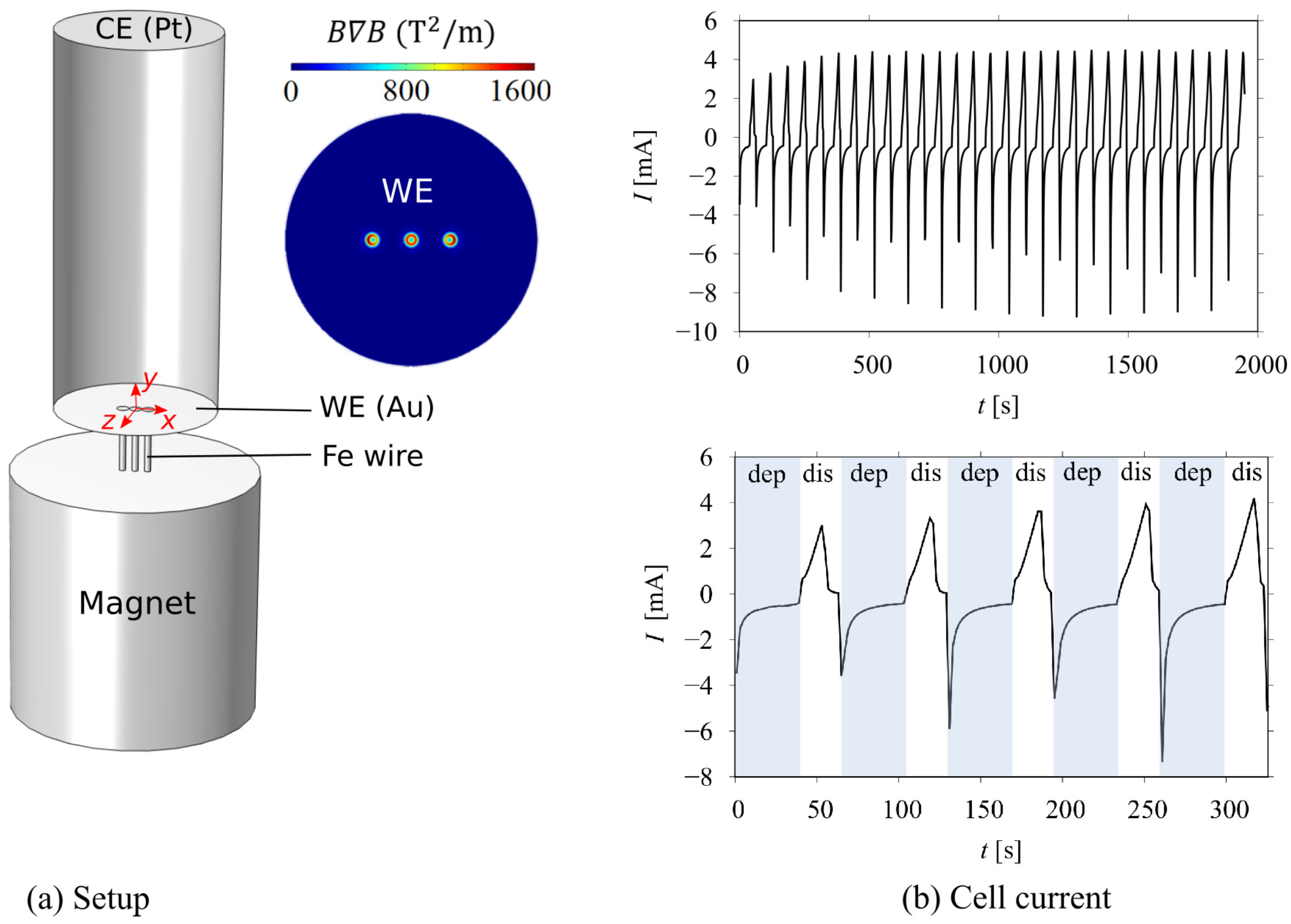
The experimental setup is adapted from previous works [10,16], and the deposition parameters are modified in order to grow larger structures. As shown in Figure 1a, a cylindrical electrochemical cell with a diameter of 13 mm and a height of 30 mm is used. The counter electrode (CE) is a Pt sheet, and the reference electrode is a MSE electrode (+650 mV vs. SHE electrode). All potentials given below refer to the MSE electrode. At the bottom of the cell, a glass disc (⌀13 mm, thickness $0.15\pm 0.02$ mm) coated with 200 nm Au is used as the working electrode (WE). The aqueous electrolyte consists of 0.01 mol/L CuSO${}_4$ and 0.1 mol/L Na${}_2$SO${}_4$ and was adjusted to a pH of 3 by H${}_2$SO${}_4$. A magnetic gradient template consisting of three Fe wires (⌀0.5 mm, height 5 mm, distance to each other 1 mm) embedded in PVC is placed below the WE. The linear arrangement of three Fe wires serves as a simple model configuration to study the interaction of fluid flow and mass transfer between neighboring ferromagnetic elements arranged e.g., in an array. At moderate computational effort for the simulations, the configuration further allows optical access for future measurements of flow and mass transfer. The magnetic gradient template is placed above a cylindrical NdFeB magnet (⌀20 mm, height 20 mm, remanent flux density 1.29 T). This magnet provides an external magnetic field of about 0.3 T near the WE, which is directed in the vertical direction, apart from slight deviations near the rim of the WE. As the Fe wires are magnetized in the magnetic field, high magnetic field gradients occur near each wire (Figure 1a). This leads to a strong magnetic gradient force, which is expected to drive an electrolyte flow and to modify the local mass transfer of the copper ions.

In the pulse-reverse plating, $E_{\mathrm{dep}}=-800$ mV is chosen as the electrode potential for the potentiostatic deposition phase, which lasts for 40 s in each pulse cycle. In the dissolution phase, the deposited Cu layer was partially dissolved using linear sweep voltammetry from $E_{\mathrm{dis}}=-400$ to $-250$ mV in 25 s, which gives a sweep rate of 6 mV/s. The measured cell current is plotted in Figure 1b as a function of time. After completing 30 plating cycles, the net charge transferred reaches $-59\mathrm{mAs}$. The height of the obtained deposit structures is measured by a profilometer, and the surface morphology is analyzed by a scanning electron microscope (SEM).

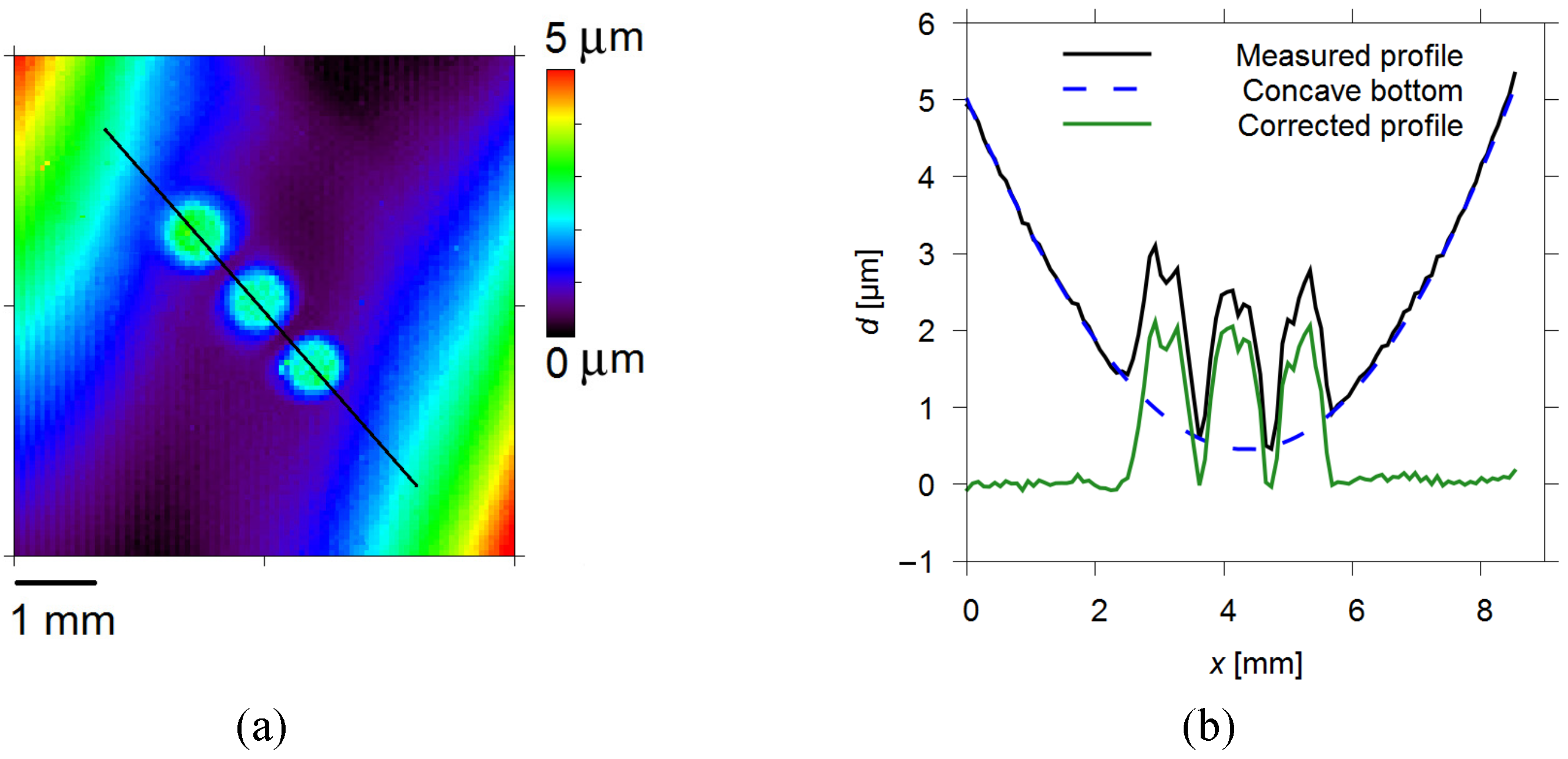
It should be noted that the substrate used for the deposition has a concave surface shape, which can not be avoided due to manufacturing details of the glass disk. As shown in Figure 2a, the concave surface shape amounts to height differences of about 5 $\mathsf{\mu }$m in the outer regions of the electrode, where the deposit thickness can safely be assumed to be negligible [16]. But the electrode bending also influences the height values measured near the Fe wires. In order to accurately determine the height of the structures, the following correction is applied along the black line that is passing the centers of the three micro-structures deposited. Here, the concave shape of the electrode prior to deposition is approximated by a parabolic function, whereby the fitting coefficients are determined from the outer thickness values measured away from the iron wires ($x\le 2\mathrm{mm},x\ge 6\mathrm{mm}$). Figure 2b shows the originally measured thickness profile (black line), the height profile prior to deposition (blue dashed line) and the corrected height profile (green line). The latter will be used for comparison with the numerical results later on.

2.2. Numerical

The numerical model applied in the simulations is described in detail in [17]. 3D Simulations are performed by using the finite element code Comsol [18] to calculate the distribution of the magnetic field, the flow velocity, the transport of metal ions, and the electric field. Specifically, a Butler-Volmer relation is applied to describe the electrode reaction kinetics:

$$j=j_{00}{\left(\frac{c_{\mathrm{s}}}{c_{\mathrm{bulk}}}\right)}^{\gamma }\left(exp\left(\frac{{\alpha }_{\mathrm{a}}F{\eta }_{\mathrm{s}}}{RT}\right)-exp\left(\frac{-{\alpha }_{\mathrm{c}}F{\eta }_{\mathrm{s}}}{RT}\right)\right),$$

(4)

with j, $j_{00}$, $c_{\mathrm{s}}$, $c_{\mathrm{bulk}}$, $\gamma$, ${\alpha }_{\mathrm{a}}$, ${\alpha }_{\mathrm{c}}$, $R,T,$ and F denoting the current density at the electrodes, the reference exchange current density, the surface and the bulk concentration of the deposited metal ions, the kinetic parameter related to the reaction order, the apparent transfer coefficients for anodic and cathodic reactions, the universal gas constant, the temperature and the Faraday constant, respectively.

The surface overpotential ${\eta }_{\mathrm{s}}$ is defined as the difference between the electric potential at the electrode surface $E_{\mathrm{e}}$ and in the electrolyte nearby ${\phi }_{\mathrm{e}}$ minus the equilibrium electrode potential ${\phi }_{\mathrm{eq}}$:

$${\eta }_{\mathrm{s}}=E_{\mathrm{e}}-{\phi }_{\mathrm{e}}-{\phi }_{\mathrm{eq}},{\phi }_{\mathrm{eq}}={\phi }_{\mathrm{eq},\mathrm{Ref}}+\frac{RT}{zF}ln\left(\frac{c_{\mathrm{s}}}{c_{\mathrm{Ref}}}\right),$$

(5)

with ${\phi }_{\mathrm{eq},\mathrm{Ref}}$ denoting the standard electrode potential [19].

The simulation parameters, e.g., the cell geometry, the electrolyte composition, and the time-dependent cell current during the pulse-reverse plating, are chosen according to the experiment. Due to the small length scale of the cone height (∼2 $\mathsf{\mu }$m) compared to that of the magnetic field gradients (∼0.5 mm), the local surface elevation of the WE caused by the growth of the conical structures is neglected in the numerical model.

An unstructured prismatic numerical mesh consisting of 4.8 million elements is used, which is refined near the iron wires to adequately resolve the high gradients of the magnetic field, the flow velocity and the concentration in these regions. Time discretization was carried out using an implicit backward differentiation formula. Each pulse cycle requires approximately 1000 time steps, with the length of each step modified by the solver based on error estimation during the calculation. Quadratic (second-order) shape functions are used for solving all the differential equations except the pressure equation, which is smoother and requires only linear (first-order) shape functions to deliver accurate results.

The material parameters used in the simulations are listed in

Table 1. Material parameters used in the simulations (room temperature).

Parameter	Value	Reference
${\chi }_{{\mathrm{Cu}}^{2+}}^{\mathrm{mol}}$ (${10}^{-8}{\mathrm{m}}^3/\mathrm{mol}$)	1.57	[20]
${\chi }_{{\mathrm{H}}_2\mathrm{O}}$ (${10}^{-6}$)	$-9.0$
${\rho }_0$ ($\mathrm{kg}/{\mathrm{m}}^3$)	1014	[21]
${\beta }_{{\mathrm{CuSO}}_4}$ (${10}^{-5}{\mathrm{m}}^3/\mathrm{mol}$)	16
${\beta }_{{\mathrm{Na}}_2{\mathrm{SO}}_4}$ (${10}^{-5}{\mathrm{m}}^3/\mathrm{mol}$)	$12.4$
$\nu$ (${10}^{-6}{\mathrm{m}}^2/\mathrm{s}$)	$1.05$
$V_{\mathrm{m},\mathrm{Cu}}$$({10}^{-6}{\mathrm{m}}^3/\mathrm{mol})$	7.11
$D_{{\mathrm{Cu}}^{2+}}$ (${10}^{-10}{\mathrm{m}}^2/\mathrm{s}$ )	$5.6$	[22]
$D_{{\mathrm{Na}}^{+}}$ (${10}^{-10}{\mathrm{m}}^2/\mathrm{s}$ )	$13.34$
$D_{{{\mathrm{SO}}_4}^{2-}}$ (${10}^{-10}{\mathrm{m}}^2/\mathrm{s}$ )	$10.04$
$z_{\mathrm{Cu}}^{2+}$	2
$z_{\mathrm{Na}}^{+}$	1
$z_{{{\mathrm{SO}}_4}^{2-}}$	−2
$j_{00}$$(\mathrm{mA}/{\mathrm{cm}}^2)$	2.5	[19,21,23,24]
${\varphi }_{\mathrm{eq},\mathrm{Ref}}$ (V)	$0.337$
$\gamma$	0.75
${\alpha }_{\mathrm{a}}$	1.5
${\alpha }_{\mathrm{c}}$	0.5

.

Based on the temporal behavior of the current density obtained in the simulations, the thickness distribution of the deposit at time t can be calculated according to Faraday’s law [19]:

$$d(x,t)=-\frac{V_{\mathrm{m}}}{zF}{\int }_0^{t}j(x,t)dt,$$

(6)

with $V_{\mathrm{m}}$ and z denoting the molar volume of the deposited metal and the charge number of the metal ion. By convention, the current density j is negative during deposition and positive during dissolution. As the computational effort for performing 3D simulations of the pulse-reverse deposition over several cycles is considerable, preliminary axisymmetric studies for a single Fe wire were performed to compare the deposit height profile obtained after 30 cycles with the values obtained when linearly extrapolating the further growth after 10 cycles. As no significant difference was found, the linear extrapolation after 10 cycles is also applied in the present 3D case to obtain the deposit height profile after 30 cycles.

3. Results and Discussion

3.1. Electrode Kinetics Related to the Cu Layer Distribution on the WE

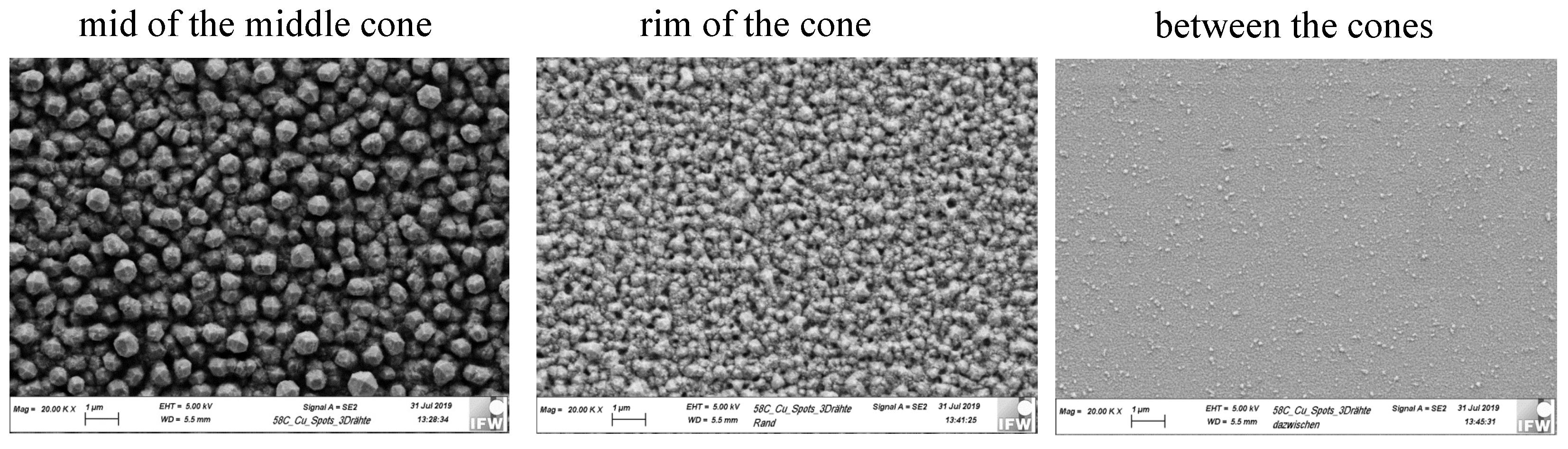
As shown in Figure 2b, after 30 cycles of pulse-reverse Cu plating, three cone-like structures of ∼2 $\mathsf{\mu }$m height are found to have grown on top of the three magnetized Fe wires in the center WE region (high-$\nabla B$ region). Figure 3 shows the surface morphology at the tip and the rim of the middle cone as well as in a region located between neighboring cones. As can be seen, the WE is completely covered by a Cu layer in the cone regions, whereby the grain size at the tip is larger than at the rim of the cone. This is related to a higher magnetic field gradient and thus a faster mass transport at the tip [25]. However, between the neighboring cones, still the Au substrate with only small Cu crystal islands can be observed. Although not shown here, photos of the WE in total also indicate that the three cones obtained after 30 cycles still remain nicely separated, and that also the outer electrode region is not covered by a Cu layer.

However, differently from what is seen in the experiment, in preliminary numerical studies it was noticed that the conical Cu structures which evolve during the cycles are not well-separated. After all cycles are completed, a thin Cu layer has formed between the neighboring cones and also in the outer region of the WE.

This difference between the simulation and the experiment might be related to a more complex reaction kinetics than given in Table 1 which always assumes a Cu substrate for simplicity. However, the kinetics of the Cu deposition and dissolution processes on the Au substrate is likely to be different. Unfortunately, a more accurate implementation of the reaction kinetics is currently not feasible due to a lack of experimental data. Therefore, in order to reduce the thickness of the Cu layer in the outer region and the regions between the cones in the simulations, an empirical approach is introduced. To slow down the deposition and to accelerate the dissolution in these regions, the exchange current density $j_{00}$ is modified as follows:

$$\begin{array}{cc}\hfill Deposition:j_{00,\mathrm{dep}}& \hfill =f_{\mathrm{dep}}·j_{00,\mathrm{Ref}},\hfill \\ \hfill Dissolution:j_{00,\mathrm{dis}}& \hfill =f_{\mathrm{dis}}·j_{00,\mathrm{Ref}}.\hfill \end{array}$$

(7)

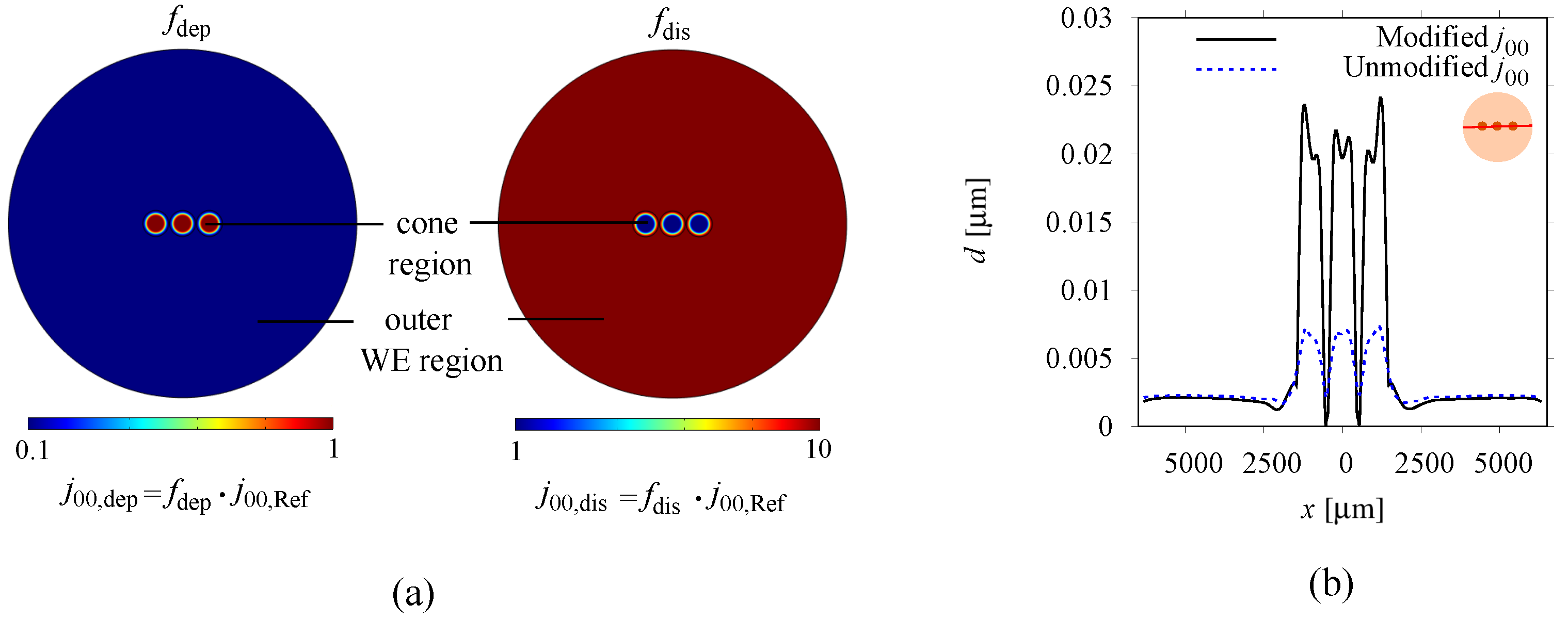
Figure 4a shows the spatial distribution of the modification factors for the deposition ($f_{\mathrm{dep}}$) and the dissolution processes ($f_{\mathrm{dis}}$) on the WE. Three circular high-$\nabla B$ regions (⌀0.97 mm) vertically aligned with the three Fe wires are defined. In these regions, where the cones are expected to grow [8], the surface can be assumed to be always covered by Cu. Thus, the electrode kinetics for Cu deposition on a Cu substrate (Table 1) fully applies, and both $f_{\mathrm{dep}}$ and $f_{\mathrm{dis}}$ are set to be unity. In the outer region and the regions between the cones, $f_{\mathrm{dep}}$ is decreased and $f_{\mathrm{dis}}$ is increased to account for the influence of the Au substrate, which promotes dissolution and retards deposition in these regions.

Figure 4b shows the distribution of the deposit layer thickness along the horizontal center line passing the three cones after 1 cycle. Compared to the simple uniform reaction kinetics, the modification of the exchange current density $j_{00}$ leads to nicely separated conical deposits, and also the deposit layer thickness in the outer region ($\mid x\mid \ge 2500\mathsf{\mu }\mathrm{m}$) is slightly reduced. We would like to mention that due to the large area fraction of the outer electrode part, the thickness of the deposit in this region strongly influences the height of the conical structures. As can be seen in Figure 4b, already the slight reduction achieved by the modified kinetics significantly enhances the cone heights. However, as still the Cu layer in the outer region cannot completely be suppressed, it is likely that the cone heights will still remain underestimated in the simulations.

3.2. Structured Deposit Growth

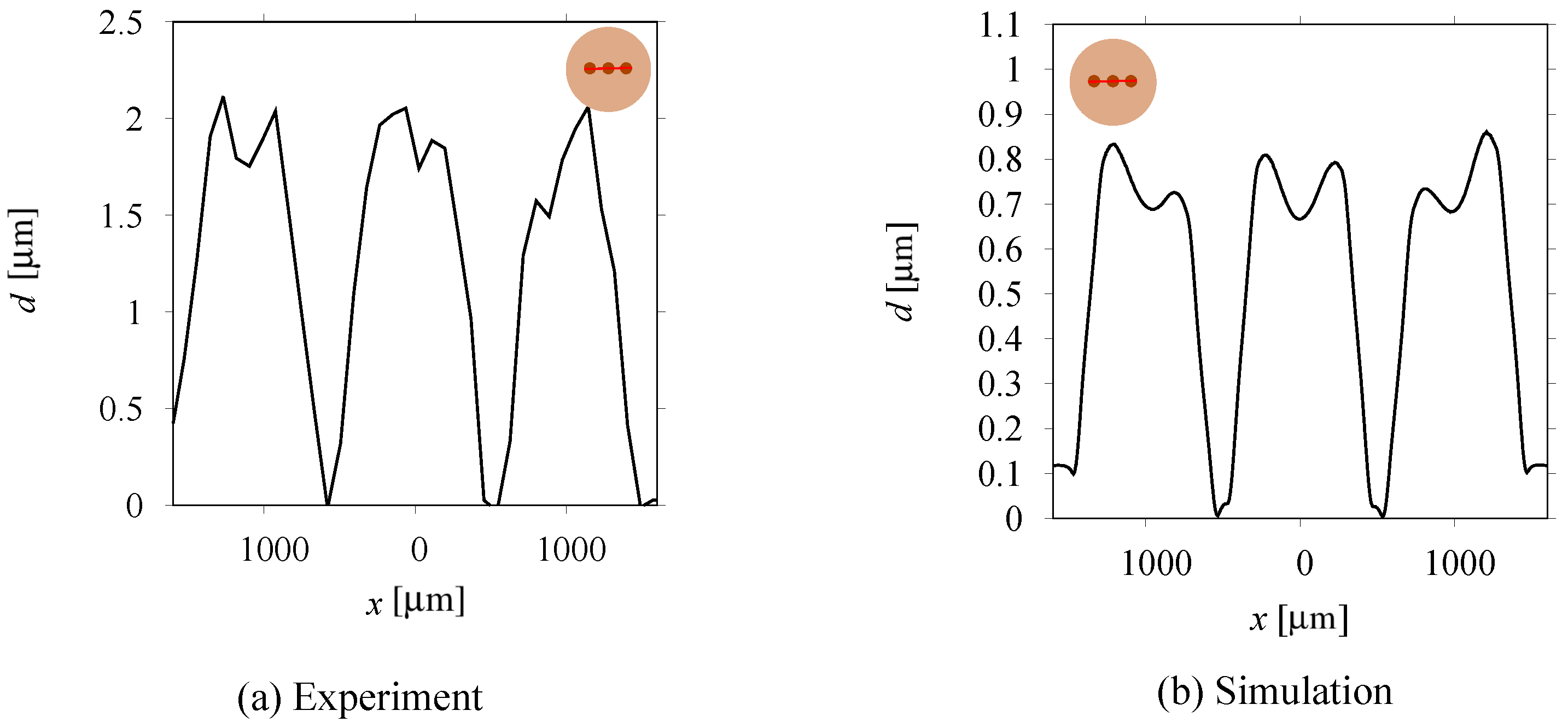
Figure 5 shows the experimental and numerical results of the deposit layer thickness after 30 cycles. Compared to the experiment, the simulation nicely qualitatively reproduces the height profile of the three cones including the small minimum in the cone centers. The largest layer thickness is found at the rim of the Fe wires where the strongest magnetic field gradients exist (see Figure 1a). Nevertheless, the cone heights obtained numerically still lack a factor of about 2.5 in height compared to the experimental results, which mainly seems to be attributed to the approximations made with respect to the unknown electrode kinetics. We remark again that even thin layers deposited radially outward account for large parts of the charge deposited in total, causing less charge flowing in the center cone regions. A more accurate implementation of the complex and partly unknown electrode kinetics in future simulations may further enhance the agreement with the experiments.

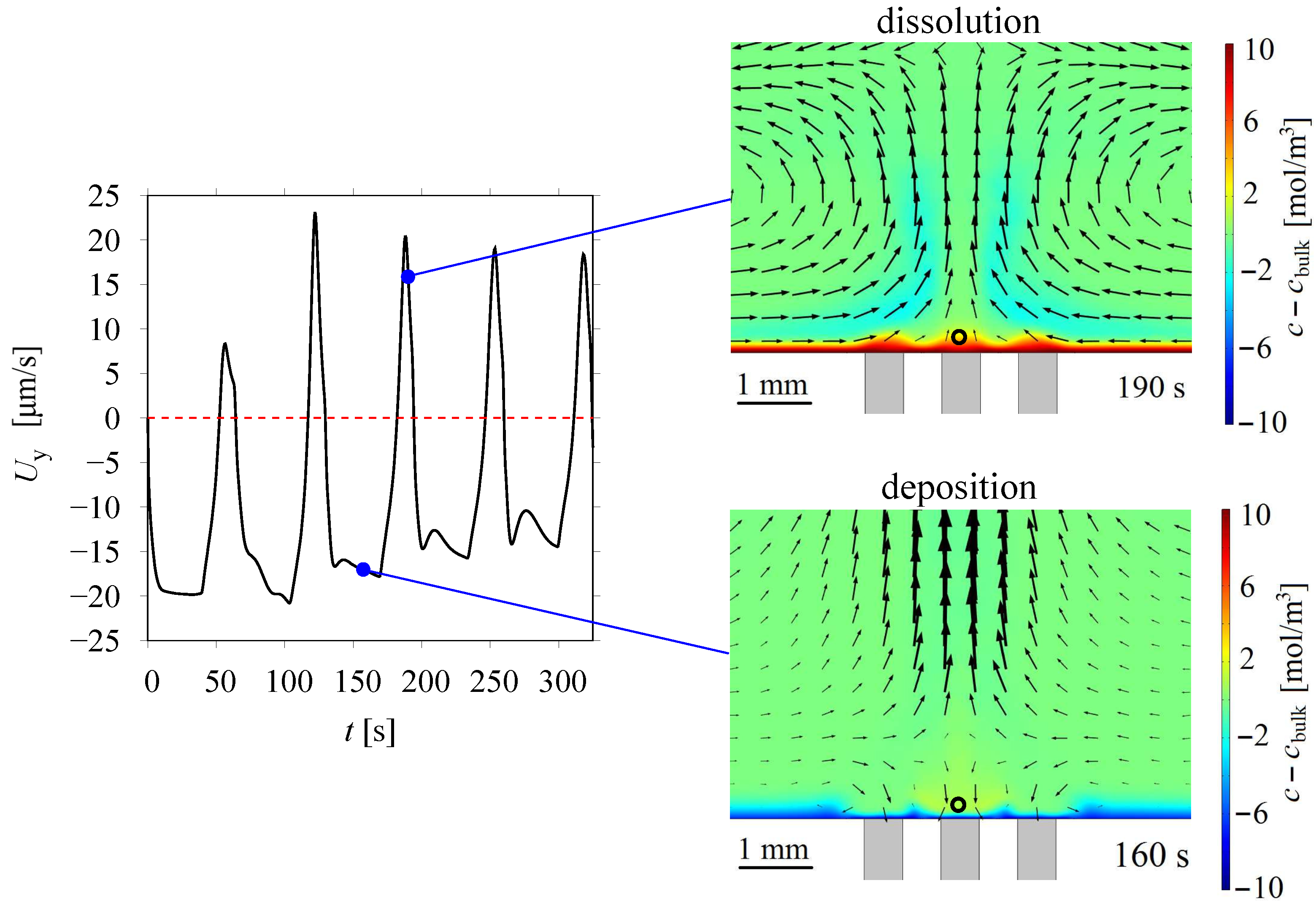
To better understand the structured deposit growth, next we analyze numerical results of the flow and the mass transfer in the electrochemical cell. Figure 6 (left) shows the temporal change of the vertical flow velocity at a point 0.1 mm above the top center of the center Fe wire, which is found to be directed downwards ($U_{\mathrm{y}}<0$) during deposition, and upwards ($U_{\mathrm{y}}>0$) during dissolution. The opposite flow directions can be interpreted as a result of the curl of the magnetic gradient force. According to Equation (2), the opposite signs of $\nabla c$ and the unchanged $\nabla \mathit{B}$ during deposition and dissolution phases result in opposite signs of $\nabla \times {\mathit{f}}_{\nabla \mathrm{B}}$, and thus of the flow forced.

During the deposition, a downward flow brings enriched electrolyte towards the electrode regions above the Fe wires, thus causing a thin concentration boundary layer with enhanced gradients (Figure 6 (right), 160 s). This small-scale local flow driven by ${\mathit{f}}_{\nabla \mathrm{B}}$ is in full agreement with the numerical findings reported in [13] and also the measurements reported in [26]. In result of the flow, the deposition rate will increase locally near each Fe wire.

During dissolution, the upward flow forced by ${\mathit{f}}_{\nabla \mathrm{B}}$ brings enriched electrolyte upwards from the surface, which is causing a thicker concentration boundary layer above the Fe wires (Figure 6 (right), 190 s). The decreased concentration gradient consequently slows down the dissolution rate in these regions. In addition, the local enrichment of Cu${}^{2+}$ ions near the Fe wires is expected to raise the reaction rate in the subsequent deposition step. Therefore, the numerical findings give further support to earlier statements that the growth mechanism in pulse-reverse deposition is due to the magnetic gradient force which drives opposite local flows that accelerate the deposition and retard the dissolution in regions of high $\nabla B$ [9,16].

Compared to potentio-/galvanostatic deposition, the additional flow generated by ${\mathit{f}}_{\nabla \mathrm{B}}$ in the dissolution phase may contribute to the higher deposit structures found in pulse-reverse plating. In addition to the magnetic gradient force, the buoyancy force may also act on the electrolyte and influence the deposit growth. For potentio-/galvanostatic deposition, as more metal ions are continuously consumed at the magnetic gradient region of the WE, here the electrolyte becomes lighter compared to other regions and is therefore accelerated upwards. This effect may counteract the local downward flow driven by the magnetic gradient force, thus hindering the structured conical growth [27]. When pulse-reverse plating is applied, however, the concentration boundary layer built during a deposition phase will be relaxed and reversed in the subsequent dissolution phase. This effect stops the upward acceleration of the electrolyte near the structure and reduces the detrimental impact of buoyancy on its further growth. This is a clear advantage of using pulse-reverse plating to produce structured deposit layers. However, as a net deposition charge is transferred during the cycles, despite the dissolution phases, with ongoing plating, similar to potentio-/galvanostatic deposition, an overall decrease of the electrolyte density occurs at the WE, which again is strongest near the growing structures. This means that after longer times compared to potentio-/galvanostatic deposition, an upward buoyancy flow may appear also in the pulse-reverse mode. In Figure 6, beside the local flow near each Fe wire, an upward global cell flow more far away from the templated electrode region can clearly be observed. The development of such a buoyancy-driven flow is likely to counteract and hinder the further growth of the conical structures. This is in line with the experimental results showing that the conical growth was found to slow down when further increasing the number of the pulse cycles.

3.3. Lorentz Force Effect

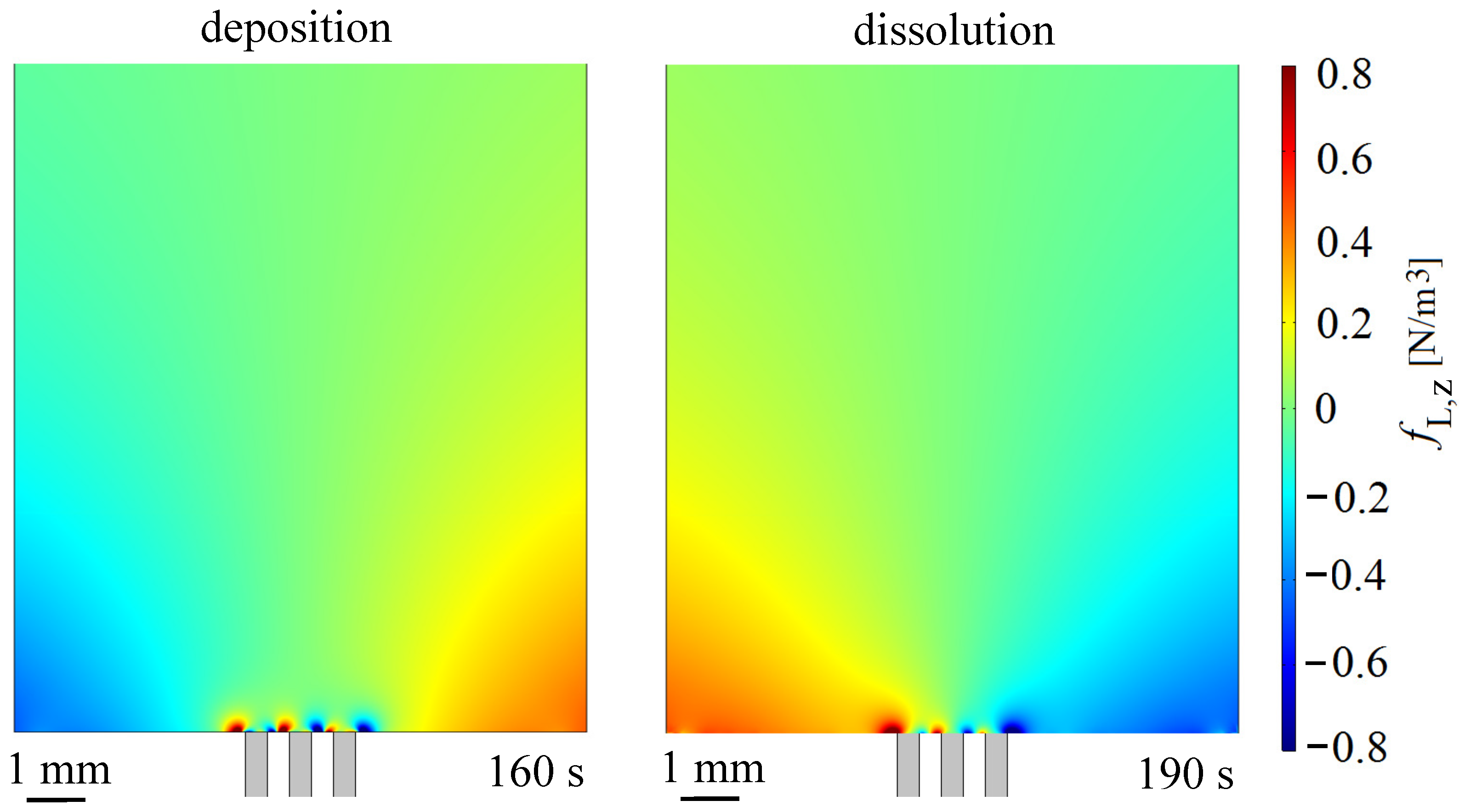
Due to the finite size of the permanent magnet, near the rim of the WE the direction of the magnetic field may deviate from the vertical direction. The horizontal components then in combination with the vertical current density cause a Lorentz force, which according to Equation (3) acts in a circumferential direction. From top view, this force is directed clockwise during deposition ($j<0$) and anti-clockwise during dissolution ($j>0$). Figure 7 shows the distribution of the paper-normal component of the Lorentz force $f_{\mathrm{L},\mathrm{y}}$ in the vertical center plane. The opposite directions of $f_{\mathrm{L},\mathrm{y}}$ observed near the electrode rim during deposition and dissolution clearly indicate that a circumferential flow of alternating direction might be driven in the cell. As can be further seen in Figure 7, also near the edges of all Fe wires Lorentz force effects are found, which originate from the local modifications of the magnetic field and the current density. However, as the forcing region is very small, related flow effects can be expected to be negligible.

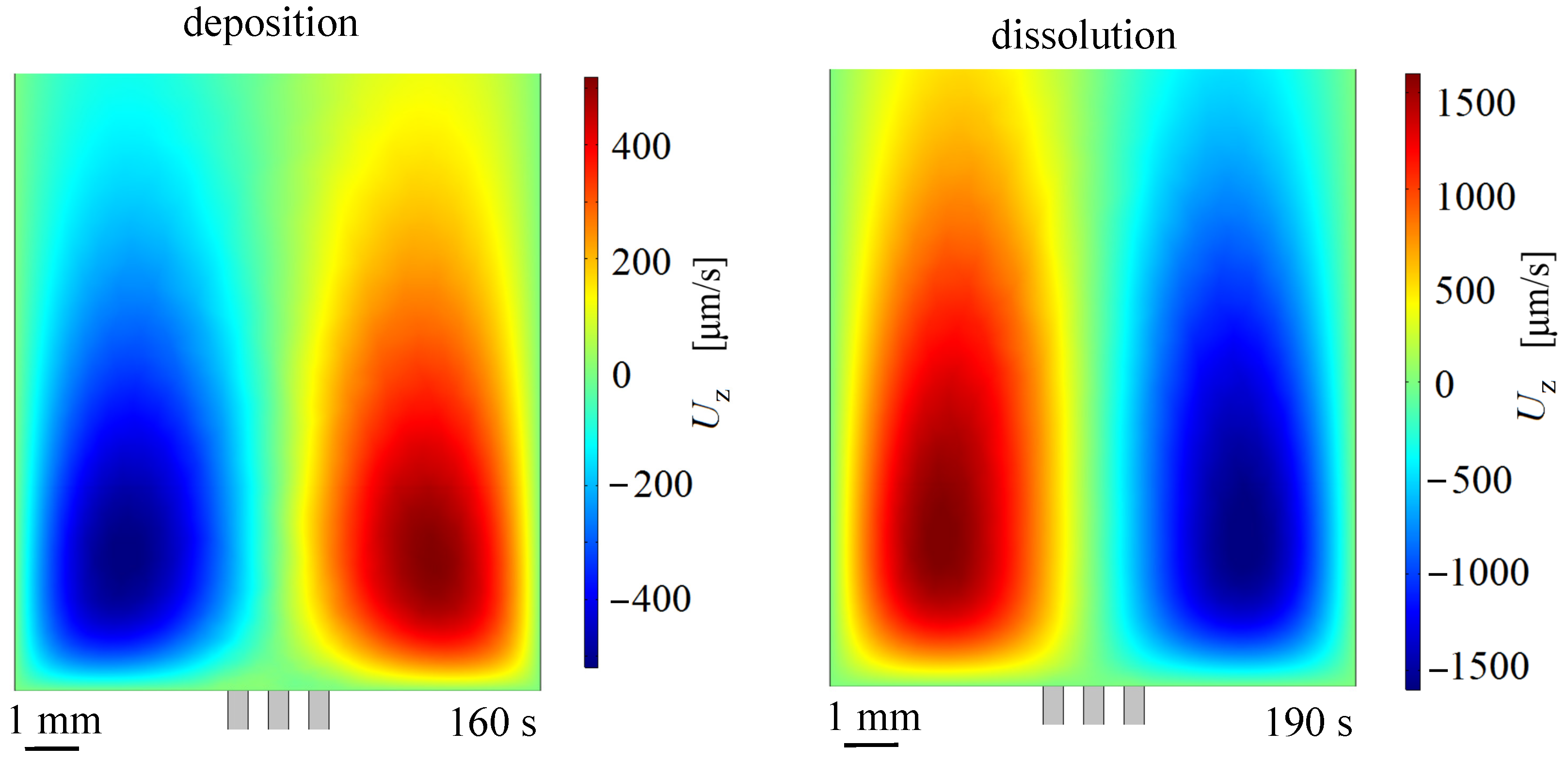
Figure 8 shows the paper-normal component of the flow velocity in the phases of deposition and dissolution. As can be seen, a circumferential global cell flow is forced, which corresponds to the direction of the strong Lorentz force that is originating from the non-vertical magnetic fields near the electrode rim. As expected, electrolyte flow resulting from the Lorentz force close by the Fe wires can not be observed. As can be further observed, the flow velocity is stronger during dissolution than during deposition, despite that the magnitudes of the cell current and ${\mathit{f}}_{\mathrm{L}}$ are almost the same at the depicted two time instants. The reason may be the higher dissolution current shortly before 190 s, which generates a stronger flow that has not yet fully decelerated, see Figure 1b.

Due to the centrifugal acceleration of the electrolyte, also a secondary flow is forced. Regardless of the rotation direction of the primary flow, the secondary flow is directed along the rotation axis towards the horizontal plane in which the primary flow is strongest. This region is found to be in the lower part of the cell (approximately 5 mm above the WE surface), see Figure 8. Thus, in addition to the solutal buoyancy effect discussed before, also the secondary flow tends to bring electrolyte upwards from the electrode. However, the horizontal flow feeding the vertical rise at the template region becomes weak due to friction near the WE surface. As can be seen in Figure 6, here the flow and the concentration boundary layer remain dominated by the influence of the magnetic gradient force that is acting near the magnetized wires.

4. Conclusions and Outlook

Cone-like Cu micro-structures were obtained from pulse-reverse plating on a planar Au electrode that is magnetically templated by three magnetized Fe wires underneath. By 3D numerical simulations the shape of the micro-structures obtained in the experiment could be closely reproduced, but the heights of the structures in the simulations were found to be lower compared to the experiment.

Nevertheless, compared to earlier investigations, the agreement was considerably improved. This was made possible partly by empirical modifications of the electrode kinetics known for copper only in order to better account for the Au electrode in the simulations. The agreement could be further improved by implementing more accurate data of the electrode kinetics in future simulations which are not yet available today. Another possible reason causing the difference between experimental and numerical results is related to a certain roughness of the micro-structure surface (see Figure 3), which was not taken into account in the simulations. Furthermore, measurements by using a microbalance could deliver additional data of the mass deposited on the WE.

The structuring of the deposit layer was found to be enabled by the magnetic gradient force, which causes a downward or upward flow during deposition or dissolution locally near each magnetized Fe wire. These local flows then alter the concentration boundary layer thickness accordingly, thereby promoting deposition and hindering dissolution to enable faster growth in these regions. The local structuring effect could be counteracted by a buoyant flow that is originating from the lower electrolyte density near the structure. However, the replenishment of the metal ions in the dissolution phases may slow down the development of the buoyant flow. Therefore, pulse-reverse plating can be expected to provide a more pronounced magnetic structuring effect when compared to potentiostatic or galvanostatic deposition.

For the experimental setup considered, slight deviations of the magnetic field vector from the vertical direction near the rim of the electrode cause a strong global Lorentz force, resulting in a circumferential primary flow and an upward secondary flow that reinforces the global buoyancy flow. In the vicinity of the WE surface, the global flow is significantly reduced due to friction, and the local flow driven by the magnetic gradient force dominates. However, as the global flow still partly counteracts the beneficial local flow, minimizing such global flow may further enhance the magnetic structuring effect. This could be realized by using larger permanent magnets or electromagnets to ensure a uniform magnetic field distribution. The global buoyancy flow could further be reduced by decreasing the cell height or by adding inert salts to the electrolyte to increase its density. Here, however, the magnetic susceptibility of the addition [6], possible changes of the electrolyte conductivity and the diffusivity of the ions have to be taken into account. Arranging the WE at the top of the cell can be expected to lead to an accumulation of depleted electrolyte near the WE. Thus, the buoyant flow would largely be suppressed. However, with growing thickness of the depleted layer the action of the magnetic gradient force reduces, and the support for local deposit growth diminishes. In order to understand these phenomena in more detail, experiments of modified setups and according simulations are required in future work.

References

- Zoski, C.G.; Liu, B.; Bard, A.J. Scanning electrochemical microscopy: Theory and characterization of electrodes of finite conical geometry. Anal. Chem. 2004, 76, 3646–3654. [Google Scholar] [CrossRef] [PubMed]
- Fujimura, T.; Kunimoto, M.; Fukunaka, Y.; Homma, T. Analysis of the hydrogen evolution reaction at Ni micro-patterned electrodes. Electrochim. Acta 2021, 368, 137678. [Google Scholar] [CrossRef]
- Arai, S.; Ozawa, M.; Shimizu, M. Communication Micro-Scale Columnar Architecture Composed of Copper Nano Sheets by Electrodeposition Technique. J. Electrochem. Soc. 2016, 164, D72–D74. [Google Scholar] [CrossRef]
- Skibińska, K.; Kołczyk-Siedlecka, K.; Kutyła, D.; Gajewska, M.; Żabiński, P. Synthesis of Co–Fe 1D Nanocone Array Electrodes Using Aluminum Oxide Template. Materials 2021, 14, 1717. [Google Scholar] [CrossRef]
- Gorobets, O.Y.; Gorobets, V.Y.; Derecha, D.O.; Brukva, O.M. Nickel electrodeposition under influence of constant homogeneous and high-gradient magnetic field. J. Phys. Chem. C 2008, 112, 3373–3375. [Google Scholar] [CrossRef]
- Mutschke, G.; Tschulik, K.; Uhlemann, M.; Bund, A.; Fröhlich, J. Comment on magnetic structuring of electrodeposits. Phys. Rev. Lett. 2012, 109, 229401. [Google Scholar] [CrossRef]
- Dunne, P.; Mazza, L.; Coey, J. Magnetic structuring of electrodeposits. Phys. Rev. Lett. 2011, 107, 024501. [Google Scholar] [CrossRef]
- Tschulik, K.; Sueptitz, R.; Koza, J.; Uhlemann, M.; Mutschke, G.; Weier, T.; Gebert, A.; Schultz, L. Studies on the patterning effect of copper deposits in magnetic gradient fields. Electrochim. Acta 2010, 56, 297–304. [Google Scholar] [CrossRef]
- Uhlemann, M.; Tschulik, K.; Gebert, A.; Mutschke, G.; Fröhlich, J.; Bund, A.; Yang, X.; Eckert, K. Structured electrodeposition in magnetic gradient fields. Eur. Phys. J. Spec. Top. 2013, 220, 287–302. [Google Scholar] [CrossRef]
- Karnbach, F.; Uhlemann, M.; Gebert, A.; Eckert, J.; Tschulik, K. Magnetic field templated patterning of the soft magnetic alloy CoFe. Electrochim. Acta 2014, 123, 477–484. [Google Scholar] [CrossRef]
- Tschulik, K.; Yang, X.; Mutschke, G.; Uhlemann, M.; Eckert, K.; Sueptitz, R.; Schultz, L.; Gebert, A. How to obtain structured metal deposits from diamagnetic ions in magnetic gradient fields? Electrochem. Commun. 2011, 13, 946–950. [Google Scholar] [CrossRef]
- Tschulik, K.; Cierpka, C.; Mutschke, G.; Gebert, A.; Schultz, L.; Uhlemann, M. Clarifying the mechanism of reverse structuring during electrodeposition in magnetic gradient fields. Anal. Chem. 2012, 84, 2328–2334. [Google Scholar] [CrossRef] [PubMed]
- Mutschke, G.; Tschulik, K.; Weier, T.; Uhlemann, M.; Bund, A.; Fröhlich, J. On the action of magnetic gradient forces in micro-structured copper deposition. Electrochim. Acta 2010, 55, 9060–9066. [Google Scholar] [CrossRef]
- Mutschke, G.; Hess, A.; Bund, A.; Fröhlich, J. On the origin of horizontal counter-rotating electrolyte flow during copper magnetoelectrolysis. Electrochim. Acta 2010, 55, 1543–1547. [Google Scholar] [CrossRef]
- Chen, Z.; Zhu, C.; Cai, M.; Yi, X.; Li, J. Growth and morphology tuning of ordered nickel nanocones routed by one-step pulse electrodeposition. Appl. Surf. Sci. 2020, 508, 145291. [Google Scholar] [CrossRef]
- Tschulik, K.; Sueptitz, R.; Uhlemann, M.; Schultz, L.; Gebert, A. Electrodeposition of separated 3D metallic structures by pulse-reverse plating in magnetic gradient fields. Electrochim. Acta 2011, 56, 5174–5177. [Google Scholar] [CrossRef]
- Huang, M.; Skibinska, K.; Zabinski, P.; Wojnicki, M.; Włoch, G.; Eckert, K.; Mutschke, G. On the prospects of magnetic-field-assisted electrodeposition of nano-structured ferromagnetic layers. Electrochim. Acta 2022, 420, 140422. [Google Scholar] [CrossRef]
- COMSOL Inc. COMSOL Multiphysics Documentation Suite V 5.6; COMSOL Inc.: Burlington, MA, USA, 2018. [Google Scholar]
- Newman, J.; Thomas-Alyea, K.E. Electrochemical Systems, 3rd ed.; John Wiley & Sons: Hoboken, NJ, USA, 2012. [Google Scholar]
- Coey, J.; Rhen, F.; Dunne, P.; McMurry, S. The magnetic concentration gradient force—Is it real? J. Solid State Electrochem. 2007, 11, 711–717. [Google Scholar] [CrossRef]
- Lide, D.R. CRC Handbook of Chemistry and Physics; CRC Press: Boca Raton, FL, USA, 2004. [Google Scholar]
- Koschichow, D.; Mutschke, G.; Yang, X.; Bund, A.; Fröhlich, J. Numerical simulation of the onset of mass transfer and convection in copper electrolysis subjected to a magnetic field. Russ. J. Electrochem. 2012, 48, 682–691. [Google Scholar] [CrossRef]
- Van Den Bossche, B.; Bortels, L.; Deconinck, J.; Vandeputte, S.; Hubin, A. Numerical steady state analysis of current density distributions in axisymmetrical systems for multi-ion electrolytes: Application to the rotating disc electrode. J. Electroanal. Chem. 1996, 411, 129–143. [Google Scholar] [CrossRef]
- Georgiadou, M. Finite-Difference Simulation of Multi-Ion Electrochemical Systems Governed by Diffusion, Migration, and Convection: Implementation in Parallel-Plate Electrochemical Reactor and Backward-Facing Step Geometries. J. Electrochem. Soc. 1997, 144, 2732. [Google Scholar] [CrossRef]
- Tschulik, K.; Kozä, J.A.; Uhlemann, M.; Gebert, A.; Schultz, L. Effects of well-defined magnetic field gradients on the electrodeposition of copper and bismuth. Electrochem. Commun. 2009, 11, 2241–2244. [Google Scholar] [CrossRef]
- Tschulik, K.; Cierpka, C.; Gebert, A.; Schultz, L.; Kahler, C.J.; Uhlemann, M. In situ analysis of three-dimensional electrolyte convection evolving during the electrodeposition of copper in magnetic gradient fields. Anal. Chem. 2011, 83, 3275–3281. [Google Scholar] [CrossRef] [PubMed]
- Huang, M.; Eckert, K.; Mutschke, G. Magnetic-field-assisted electrodeposition of metal to obtain conically structured ferromagnetic layers. Electrochim. Acta 2020, 365, 137374. [Google Scholar] [CrossRef]
Figure 1.
(a) Sketch of the electrochemical cell with the planar WE that is magnetically templated by three magnetized iron wires. The distribution of the magnetic gradient term on the WE is shown on the right (zoomed top view). (b) Cell current measured in experiments. Top: all 30 cycles. Bottom: the first 5 cycles.
Figure 2.
(a) Result of the topology measurement. The concave shape can be clearly seen. (b) The originally measured deposit profile along the line passing the three micro-structures, the concave substrate shape obtained from fitting (see text), and the corrected deposit thickness.
Figure 3.
Morphology of the surface at the mid of the middle cone (left), the rim of the middle cone (middle) and in a region between the cones (right) after 30 cycles.
Figure 4.
(a) Distribution of the modification factors for the exchange current density . (b) Deposit layer thickness along the horizontal center line passing the three cones after 1 cycle for modified and unmodified .
Figure 5.
Deposit layer thickness along the horizontal center line passing the three cones in (a) the experiment and (b) the simulation. is set to be at the bottom of the cones in both cases.
Figure 6.
(Left) Vertical flow velocity at a point 0.1 mm above the top center of the middle Fe wire (indicated by the black circle in the right subfigures) as a function of time. A dashed line at = 0 is added. (Right) Distribution of the concentration variation in the center vertical plane at 160 s (deposition) and 190 s (dissolution). Black arrows represent velocity vectors.
Figure 7.
Lorentz force component in paper direction in the vertical center plane passing the three Fe wires at 160 s (deposition) and 190 s (dissolution).
Figure 8.
Velocity component in paper direction in the vertical center plane passing the three Fe wires at 160 s (deposition) and 190 s (dissolution).
Publisher’s Note: MDPI stays neutral with regard to jurisdictional claims in published maps and institutional affiliations. |
© 2022 by the authors. Licensee MDPI, Basel, Switzerland. This article is an open access article distributed under the terms and conditions of the Creative Commons Attribution (CC BY) license (https://creativecommons.org/licenses/by/4.0/).
Share and Cite
MDPI and ACS Style
Huang, M.; Uhlemann, M.; Eckert, K.; Mutschke, G. Pulse Reverse Plating of Copper Micro-Structures in Magnetic Gradient Fields. Magnetochemistry 2022, 8, 66. https://0-doi-org.brum.beds.ac.uk/10.3390/magnetochemistry8070066
AMA Style
Huang M, Uhlemann M, Eckert K, Mutschke G. Pulse Reverse Plating of Copper Micro-Structures in Magnetic Gradient Fields. Magnetochemistry. 2022; 8(7):66. https://0-doi-org.brum.beds.ac.uk/10.3390/magnetochemistry8070066
Chicago/Turabian StyleHuang, Mengyuan, Margitta Uhlemann, Kerstin Eckert, and Gerd Mutschke. 2022. "Pulse Reverse Plating of Copper Micro-Structures in Magnetic Gradient Fields" Magnetochemistry 8, no. 7: 66. https://0-doi-org.brum.beds.ac.uk/10.3390/magnetochemistry8070066
Note that from the first issue of 2016, this journal uses article numbers instead of page numbers. See further details here.