Grid Impacts of Uncoordinated Fast Charging of Electric Ferry

1
Department of Electrical and Electronic Engineering, Primeasia University, Dhaka 1213, Bangladesh
2
School of Engineering and Technology, Central Queensland University, Norman Gardens, QLD 4701, Australia
3
School of Maritime Electrical Engineering, University of Tasmania, Hobart, TAS 7005, Australia
*
Author to whom correspondence should be addressed.
Batteries 2021, 7(1), 13; https://0-doi-org.brum.beds.ac.uk/10.3390/batteries7010013
Submission received: 29 December 2020
/
Revised: 19 January 2021
/
Accepted: 25 January 2021
/
Published: 17 February 2021
Abstract
:The battery energy storage system (BESS) is an indispensable part of an electric fleet (EF) which needs to be charged by electricity from local grid when the fleet is in the dockyard. The uncoordinated fast charging of BESS in Grid to Ferry (G2F) mode imposes sudden increments of load in the power grid, which is analyzed by a simulated model of grid connected marine load. The probable impact on system stability is examined by MATLAB Simulink and Power World Simulator based models. According to simulation results for IEEE 5 bus system, voltage unbalance factors are 0.01% and 200% for all buses at fundamental and third harmonics frequencies, respectively. The total harmonic distortion (THD) at fundamental frequency becomes 0.16%, 0.16%, and 0.18%, respectively, for three cases. The transient, voltage reactive power (V-Q), and voltage real power (V-P) sensitivity analysis are performed for 7 bus system with load increment contingencies. According to simulation results, the V-Q sensitivity for the assigned contingency is increased by the addition of a shunt generator to the load bus with lowest bus voltage. In case of V-P sensitivity for the selected contingency, the load buses share power among them, and the nose point is attained at maximum shift of power with high V-Q sensitivity.
1. Introduction
For mitigating the harmful environmental effects of greenhouse gas (GHG), which is emitted by conventional fossil fuels, the utilization of renewable resources is increasing day by day. The transport sector is one of the prime emitters of GHG and was responsible for 35% of the total energy consumed in 2014, of which 21% corresponded to passenger transport with an average consumption of 1.9 MJ/km [1]. According to the International Maritime Organization (IMO), the carbon dioxide emission from shipping is equal to 2.2% of the global human made emissions in 2012, which is expected to rise to 50–250% by 2050 if no action is taken for reducing emission [2,3]. The battery powered electric fleet (EF) can be an alternate option for conventional diesel engine ferry for reduction of greenhouse gas. Like electric vehicles (EV), further research on charging technologies of EFs is required. There are basically three EV charging setups which can also be applicable for EF. The first setup is of 120 V AC with 6.5 A per hour charging, the second setup comprises of 220/240 V AC with up to 30 A per hour charging, and the third setup is up to 800 V DC with up to 300 A per 20–30 min charging [4,5]. Generally, the DC charging is called fast charging, and various charging methods and algorithms have been proposed for improving charging time, efficiency, and life cycle of different batteries in various studies. These methods include Constant Current (CC), Constant Voltage (CV), CC-CV, double loop control, fuzzy logic control, boost charge, pulse charge, droop control, quadratic optimization, gradient optimization, linear programming, game theory, and artificial neural network [6,7]. The most recommended and popular method for battery charging is CC-CV charging, which consists of trickle charge, constant current, constant voltage, and charge termination [8,9].
Like EV, when EF is connected to a power outlet, it can operate in two modes, (1) charging mode, which is called Grid to Ferry (G2F) mode, and (2) discharging mode, which is called Ferry to Grid (F2G) mode [10]. However, in case of using EF in F2G mode depends on availability of EF in cold ironing stage. Like EV, EF can act as a fast charging load for G2F mode, whereas it acts as a power source in case of F2G mode [11,12]. The impacts of fast charging EF load on local grid mainly depends on number of connected EF to grid and charging and discharging characteristics of battery. The battery is charged either in coordinated mode or uncoordinated mode [13]. In coordinated charging, charging is done during off peak hours of the day when the load demand is low whereas in uncoordinated charging, the charging is done irrespective of load demand during any time of the day [14,15]. Moreover, smart charging infrastructure is used by coordinated charging which helps in minimizing load burden on existing distribution system [16]. Like Vehicle to Grid (V2G), F2G helps in retaining system stability by regulation of active power, supporting reactive power, load balancing, peak load shaving, and minimization of harmonics [17,18]. With increasing integration of green electricity from renewable sources to grid, a battery energy storage system (BESS) provides ancillary services like spinning reserve, voltage, and frequency control [19]. Degradation of battery, upgradation of the existing grid, and extensive communication between EF and grid are challenging issues for F2G [20,21]. For uncoordinated charging, a fast charging battery generally consumes a large amount of power over a short time, and probable impacts of that on the grid are an increase of peak load demand with fluctuations of system voltage and frequency, which affect voltage regulation [22], increment of power system losses [23], and overloading of distribution transformers, distribution lines, and cables [24,25]. The power system stability greatly depends on the nature of the load, therefore an accurate load model for a fast charging battery is required to identify its impact on the grid [26].
Though several research works have so far been conducted on impacts of fast charging of EV on electricity grid, very few similar research works have been conducted for EF. In this paper, a simulated model of grid interactive marine electrical system is designed by MATLAB Simulink in order to identify probable impacts of fast uncoordinated charging on electricity grids. Since the BESS of EF is charged without a smart coordinated charging schedule, the fast-charging consumes large amounts of power within a short time, which may create instability in the power system. Section 2 discusses the probable impacts on power system stability due to uncoordinated fast charging in terms of the simulated model. The intermittent green electricity from photovoltaic (PV) and uncoordinated fast charging of EF causes instability in the electricity grid. The probable impacts on system stability due to sudden load increment is analogous to the inclusion of uncoordinated fast charging load to the power system is analyzed by simulated models of 5 bus and 7 bus networks. In Section 2.1, the variation in system voltage and frequency are investigated in terms of voltage unbalance factor and total harmonic distortion (THD) by a MATLAB Simulink model of an IEEE 5 bus system. The transient stability, voltage real power (V-P) and voltage reactive power (V-Q) sensitivity analysis for different contingency scenarios are performed for a Power World Simulator based 7 bus system in Section 2.2. A probabilistic simulation analysis is performed in this paper for identifying impacts of uncoordinated fast charging on electrical power systems. Finally, the paper ends with a discussion in Section 3, where the findings of this paper are included, along with shortfalls and future work.
2. Simulation Results on Impacts of System Stability
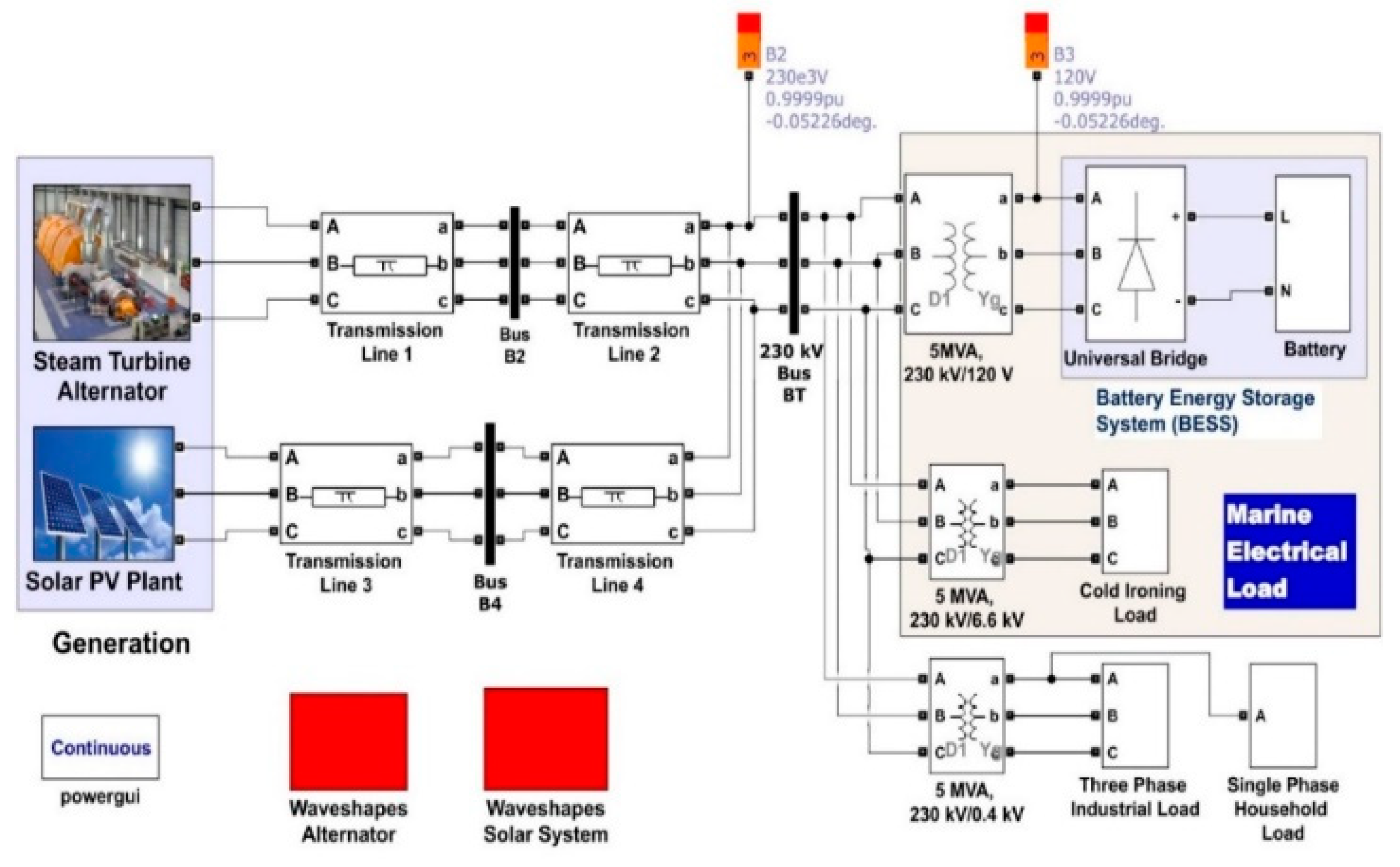
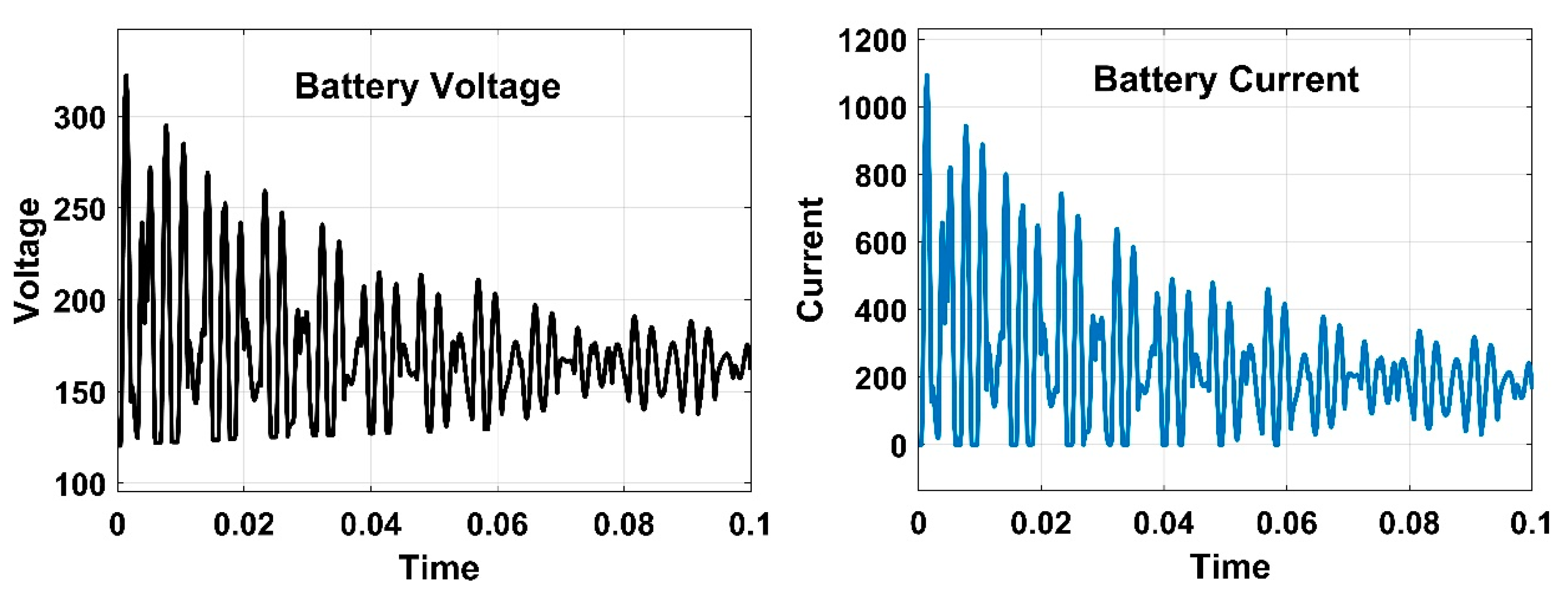
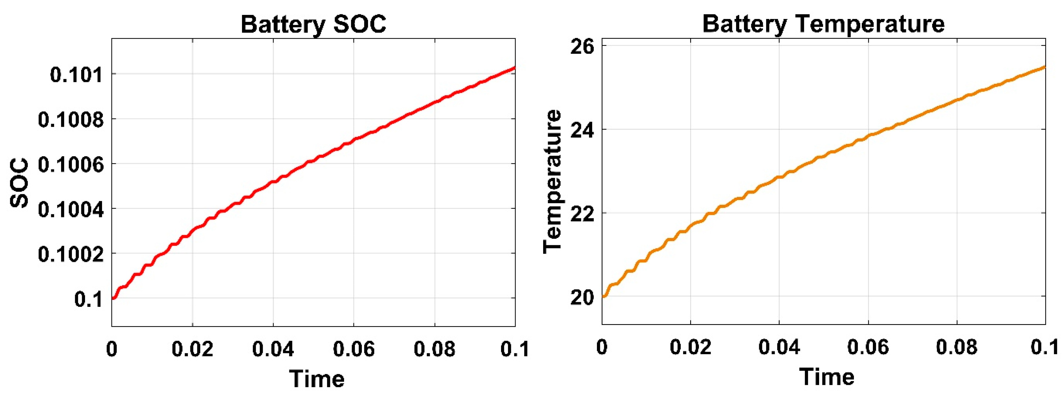
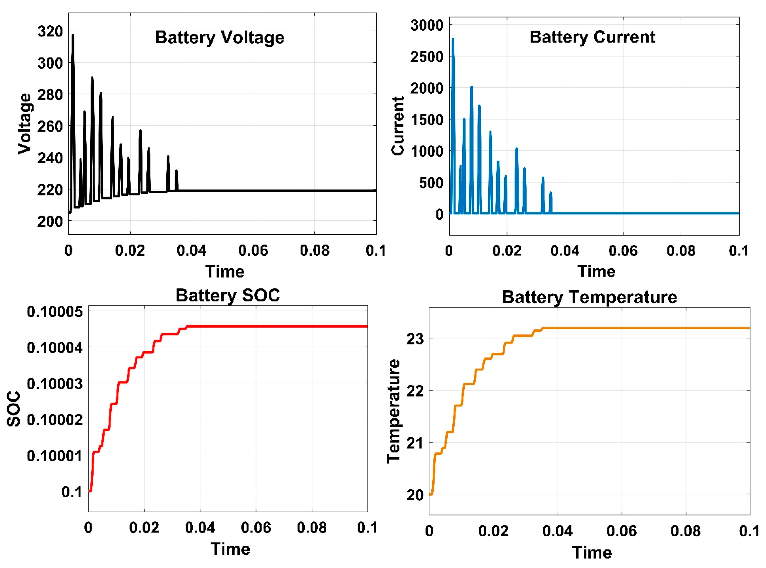
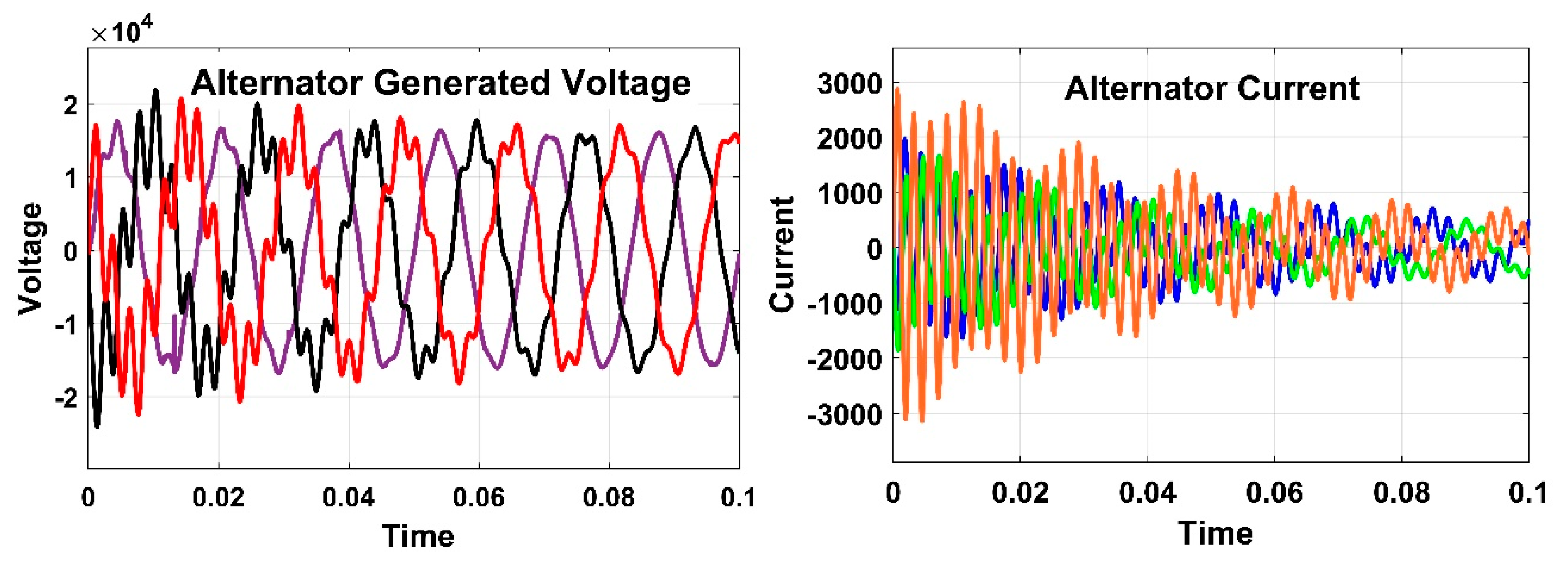
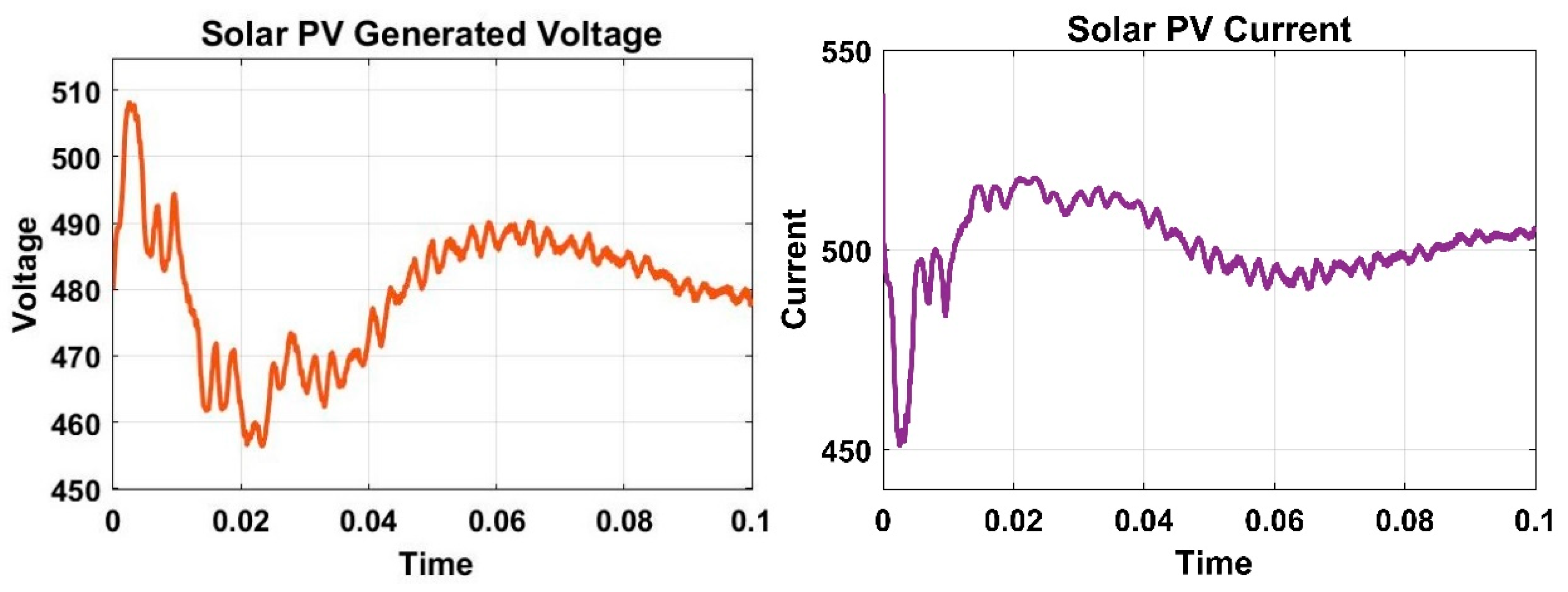
A simulated model of grid connected marine electrical load is designed by MATLAB Simulink for identifying uncoordinated slow and fast charging characteristics of BESS is shown in Figure 1. The electrical load for a docked marine vessel is comprised of an on-board BESS, which consumes electricity from a 120 V bus, whereas cold ironing load (both single and three phase resistive and inductive load) consumes electricity from a 6.6 kV bus. The electricity generation comprises of steam turbine-based alternator of 100 MVA, 11kV, and solar PV of 240 kW, 480 V. Two generation buses are B1 and B4, which are connected to 230 kV, 60 Hz transmission bus, BT. The charging of a battery depends on the initial state of charging (SOC) and battery capacity. Therefore, the initial charging voltage and current varies significantly with slow and fast charging of the battery. According to the simulation results, in case of slow charging of the battery with 120 V and 6.5Ah supply, the initial charging voltage and current become 350 V and 1050A with 10% initial SOC. The voltage and current are reduced gradually with increasing SOC. The initial ambient temperature of the battery is considered 20 °C, which increases with charging. Figure 2 shows the battery voltage, current, SOC, and temperature curves during slow charging for a simulation time of one hour. In case of fast charging of the battery with 200 V and 50 Ah supply, the initial charging voltage and current become 318 V and 2800 A, respectively, with 10% initial SOC. The battery is fully charged in a short time in comparison to that of slow charging. Figure 3 shows the battery voltage, current, SOC, and temperature curves during fast charging for a simulation time of one hour. The generation pattern of the steam turbine alternator and solar PV with corresponding voltage and current are shown in Figure 4 and Figure 5, respectively. The uncoordinated fast charging of BESS of EF imposes sudden load increment in the power system, and its probable impacts are discussed with 5 bus and 7 bus systems in the following sections.
2.1. Impacts on Voltage Stability
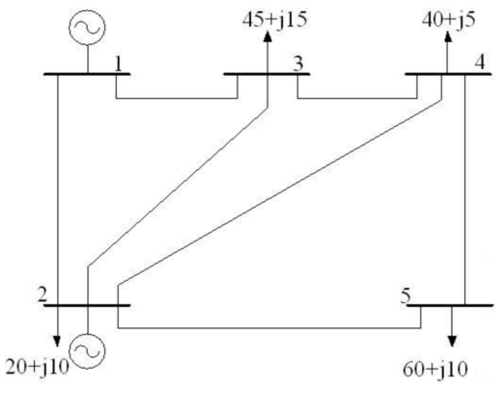
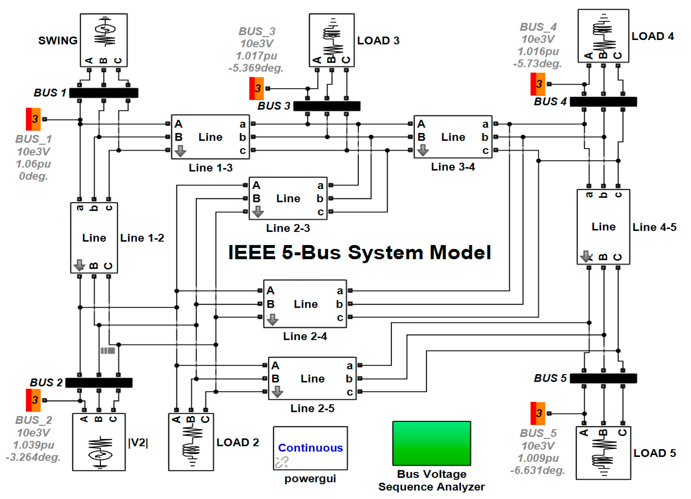
The voltage unbalance factor and THD are two important aspects for voltage stability of the power system. In this paper, these two aspects are considered for finding probable impacts on grid voltage stability due to uncoordinated fast charging of BESS. The sudden increment of load due to BESS charging is analyzed by load flow analysis of IEEE 5 bus in a MATLAB Simulink environment. Three cases are considered for replicating the impacts on bus voltage due to integration of charging load of EF with local grid. For simplicity, the EF charging load is considered as a PQ (Real Power Reactive Power) type load, and three load increment cases are created by percentage increments of load for buses. In case 1, 25% additional load is added to the network, whereas 50% and 75% additional loads are added in cases 2 and 3, respectively. Figure 6 and Figure 7 represent the single line diagram and simulated model of IEEE 5 bus system, where buses 1 and 2 are slack and source buses, respectively, whereas buses 3, 4, and 5 are load buses. Though bus 2 is the source bus, load is added to this bus and the increment of load is equally distributed to all buses except the slack bus. The base voltage and fundamental frequency are considered as 25kV and 60 Hz. The sequence analyzer block is used for calculating magnitude and angle of positive sequence, negative sequence, and zero sequence voltages of respective phase voltages of different buses for calculating the voltage unbalance factor. The voltage unbalance factor is defined as the ratio of the negative sequence voltage component to the positive sequence voltage component, which is represented mathematically by Equation (1) [27].
where, V1 and V2 represent the positive and negative sequence voltage components, respectively.
The results of load flow analysis for different cases are represented in Table 1, Table 2, Table 3 and Table 4. The voltage unbalance factor is calculated for all buses at fundamental frequency and third harmonics frequency, which are 0.01% and 200%, respectively, for all cases. The voltage unbalance factor increases with higher order harmonics. According to load flow analysis, the bus voltages of the actual IEEE 5 bus system are within 1 pu, whereas voltages of all buses except 5 are within 1 pu for case 1. The bus voltages of 1 and 2 are within 1 pu whereas bus voltages of 3, 4, and 5 are below 1 pu for cases 2 and 3. Since bus 1 is the slack bus, therefore its voltage remains the same (1.06 pu) irrespective of increment of load, and the generation of slack generator also increases accordingly with the load demand.
The THD is a measurement of the harmonic distortion present, which is defined as the ratio of the square root of sum of voltages for different harmonic components to the voltage of fundamental frequency. Generally, the THD is expressed in percentage or decibel. The THD at fundamental frequency can be represented by Equation (2).
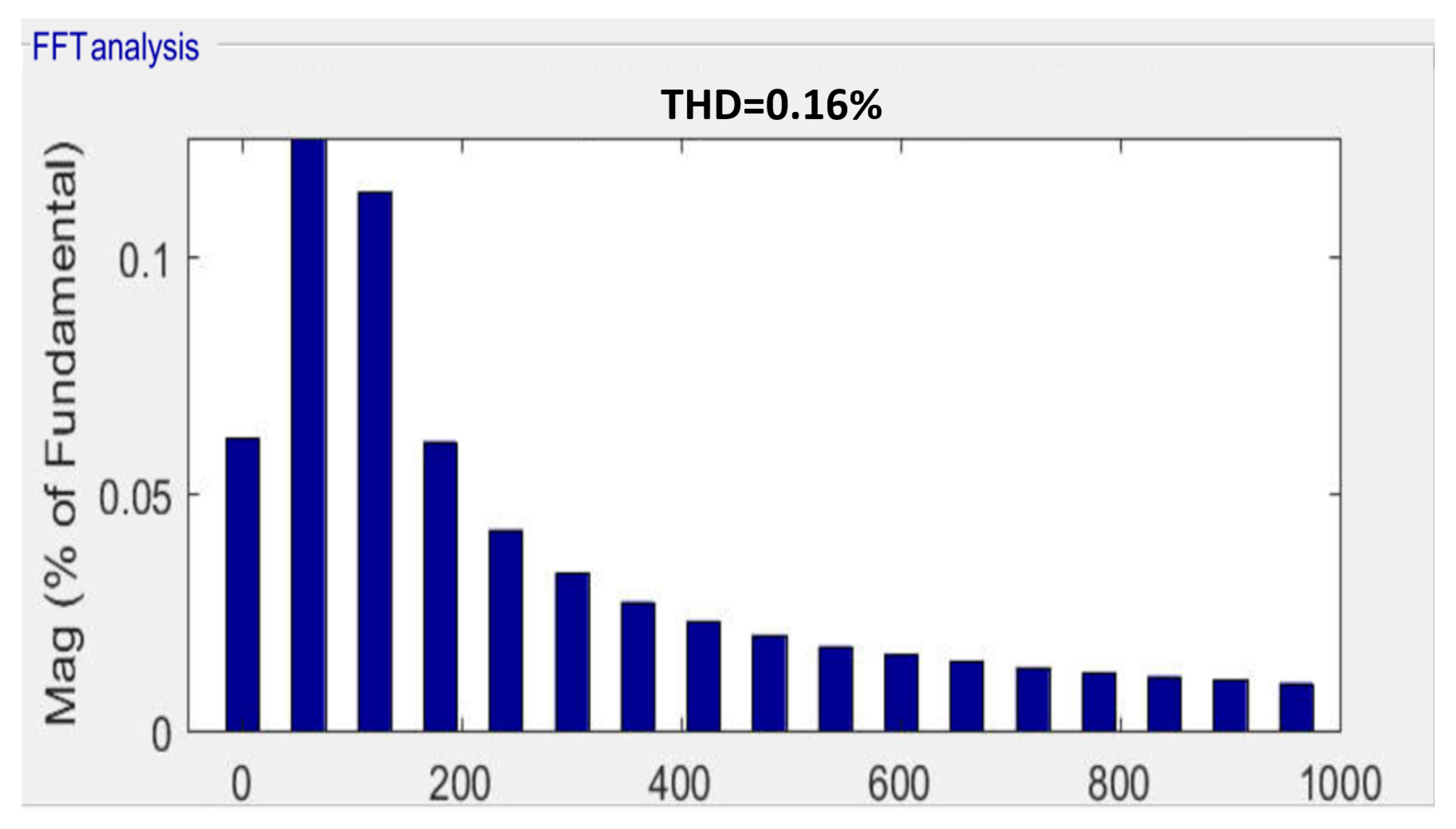
The allowable value of THD in percentage for different voltage level according to IEEE 519-2014 standards is mentioned in Table 5. The THDs at fundamental frequency are 0.16%, 0.16%, and 0.18%, respectively, for three cases, while the THD is 0.16% for the actual 5 bus system before increasing the load, which is represented in Figure 8.
2.2. Transient Stability, V-P and V-Q Sensitivity Analysis
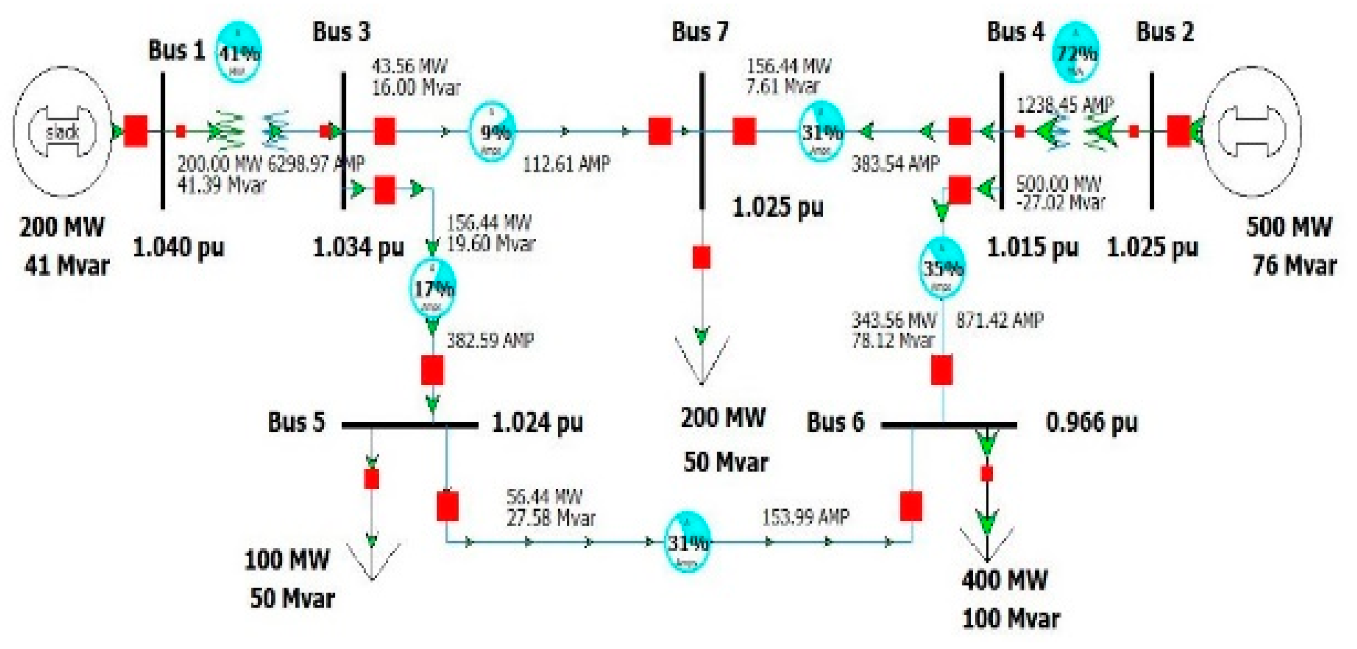
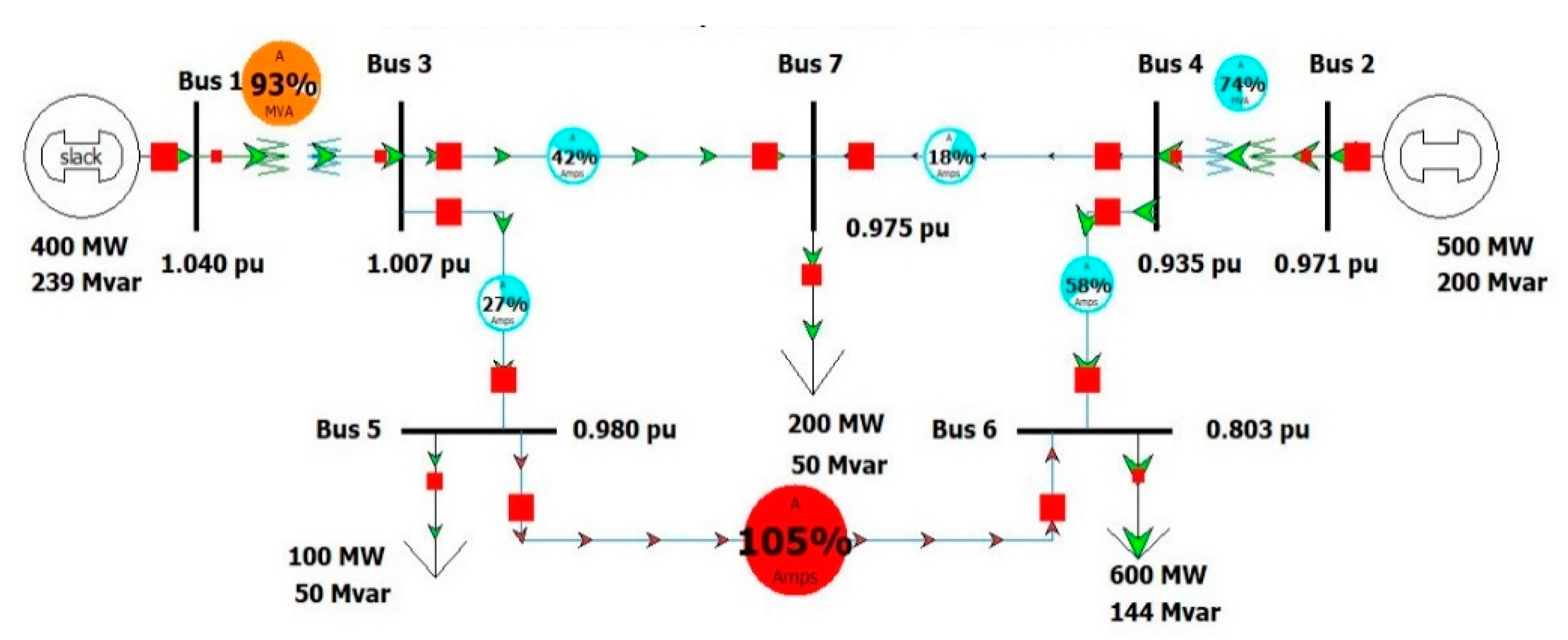
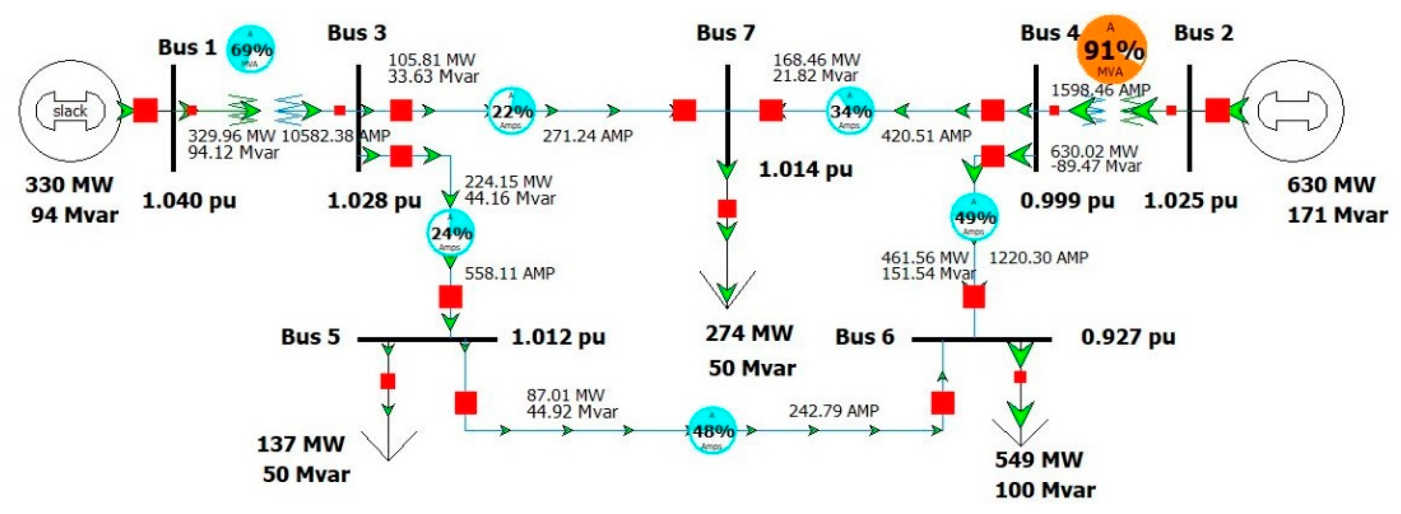
The transient stability analysis, V-P, and V-Q sensitivity analysis are generally suitable for identifying possible impacts on bus voltage and frequency in case of sudden load change. The impacts on the grid for sudden load change due to uncoordinated fast charging of BESS is analyzed by a Power World Simulator based 7-bus network, which is comprised of two source buses (1 and 2), three load buses (5, 6, and 7), and two transmission buses (3 and 4). Figure 9 shows the 7-bus network with base MVA is 1000 MVA, and nominal voltage for source buses and load buses are 18 kV and 230 kV, respectively.
2.2.1. First Contingency Scenario: Increment of 100% Load at Buses 5 and 7
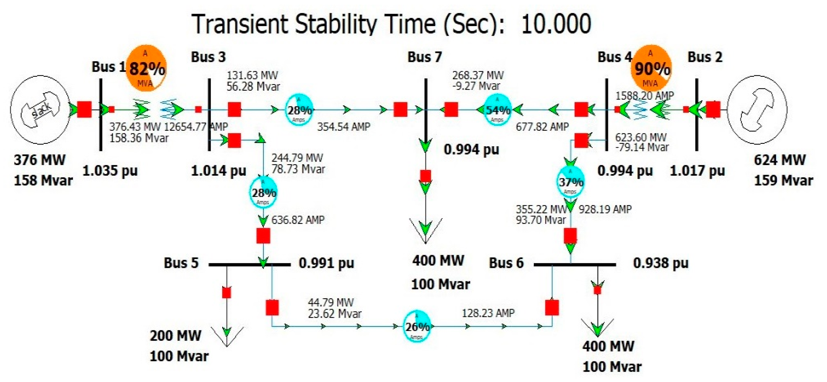
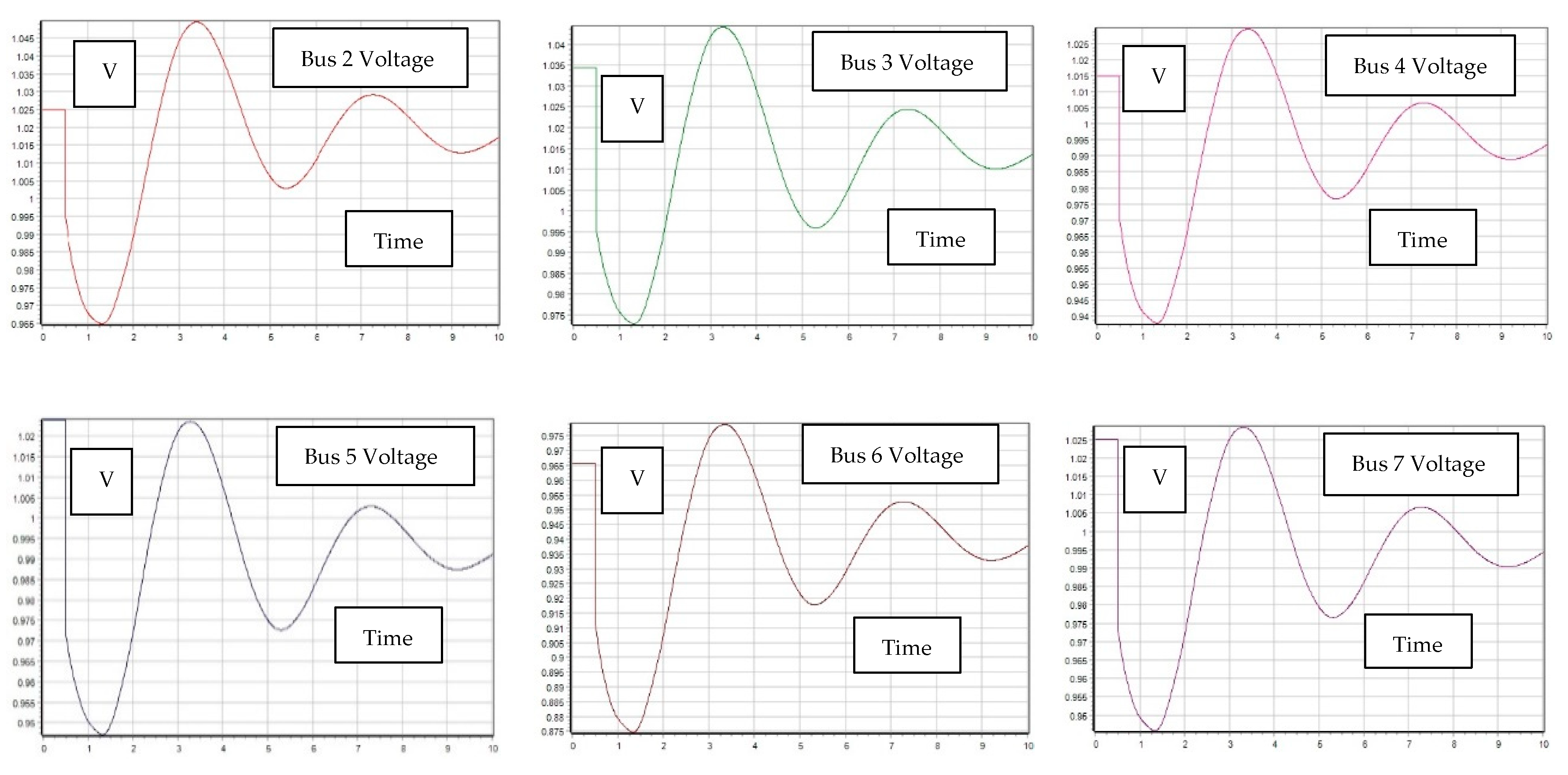
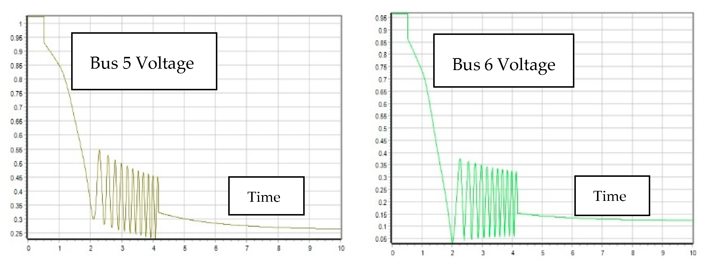
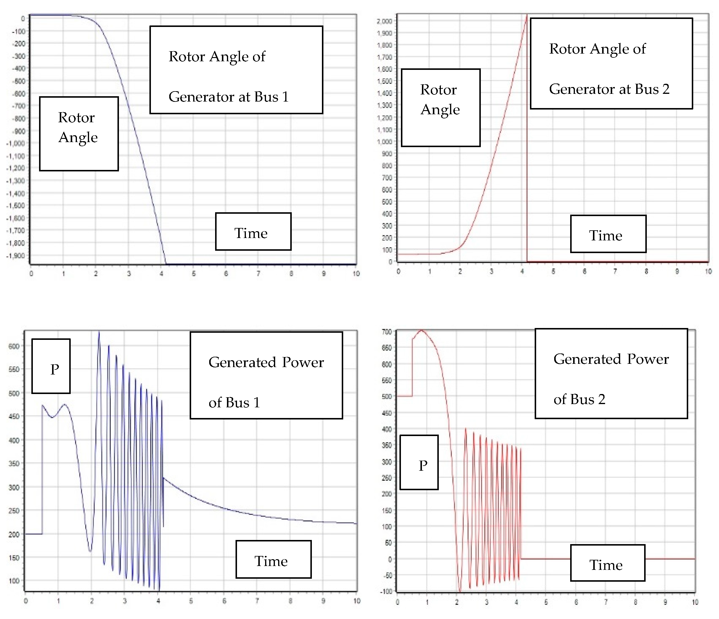
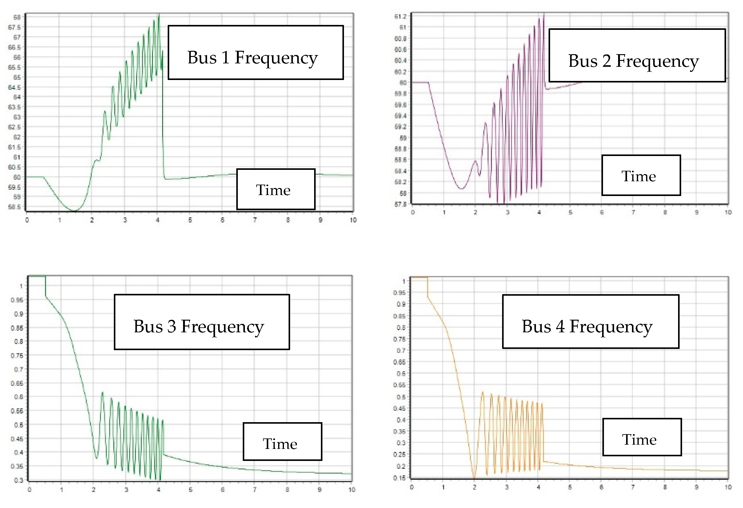
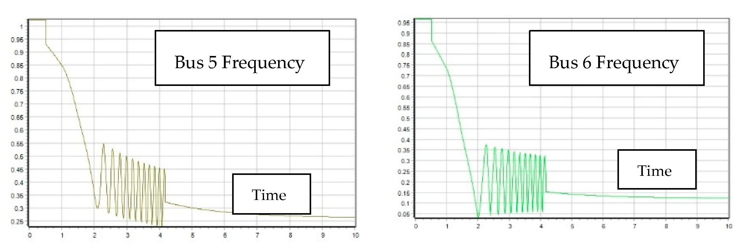
In case of transient stability analysis, two contingency scenarios are created by 100% increment of load with respect to the base case for buses 5 and 7. The system parameters like bus voltage, bus frequency, and variation of rotor angle with voltage for slack generator are investigated according to contingency conditions. Figure 10 shows the transient stability analysis of the 7 bus system network. The initial load of buses 7 and 5 are 200 MW, 50 Mvar and 100 MW, 50 Mvar, respectively, which are increased to 400 MW, 100 Mvar and 200 MW, 100 Mvar, respectively, for the first transient contingency scenario. The transformers connected to buses 1 and 2 are rated as 500 MVA and 700 MVA, respectively. Figure 10 shows the power flow scenario for a simulation time of 10 s where the transformers at buses 1 and 2 are 82% and 90% loaded, respectively. The voltages of buses 4, 5, 6, and 7 go below 1 per unit, which was initially set to 1 per unit before sudden increment of load within 0.5 s. The system performance under transient stability conditions can be analyzed from bus voltage and system frequency with corresponding rotor angle and generated voltage. Figure 11 and Figure 12 show bus voltages and frequencies of different buses where the bus voltages fluctuate continuously after 0.5 s when the loads in buses 5 and 7 are suddenly increased. Except for slack bus voltage, all other bus voltages drop to their previous values of steady state condition, which is shown in Figure 9. In the figures, voltage in per unit and frequency in Hz are represented along x axis, whereas the simulation time in seconds is represented along y axis.
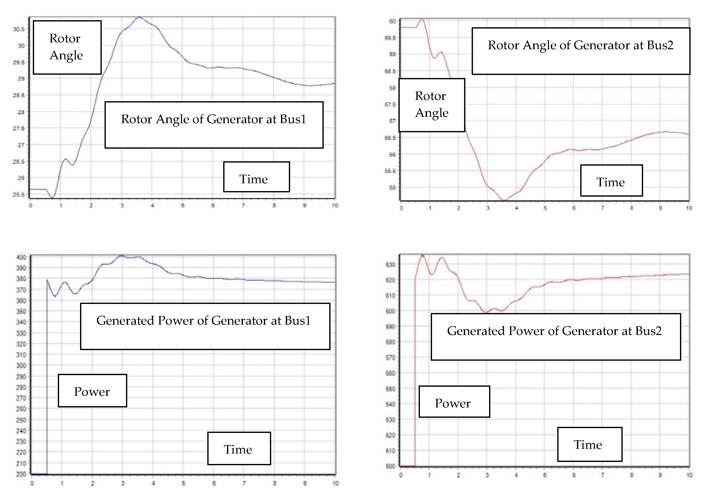
The generated power in MW with respect to time of each generator is represented in the Figure 12. The frequency at different buses fluctuates with change in bus voltages, which is shown in Figure 13. The bus frequency drops to 58.4 Hz at around 2.4 s after sudden increase in load at 0.5 s. Then, gradually, the bus frequency increases to its steady state frequency of 59.48 Hz, which is the same as that of the base case simulation of Figure 9. The rotor angle and generated power of the alternator also responded to sudden load increment, which is shown in Figure 13. With sudden increment in load at 0.5 s, the generated voltage drops below the rated value for both generators at 1.2 s, and then increases above the rated value at 3.2 s. Finally, the generated voltage reaches to a rated steady state value after continuous variations of voltage. The rotor angle of each generator oscillates with respect to time and then reaches to an equilibrium point for maintaining system stability. The rotor angle follows the generated power according to the swing equation of synchronous machine.
2.2.2. Second Contingency Scenario: Increment of 150% Load for Buses 5 and 7
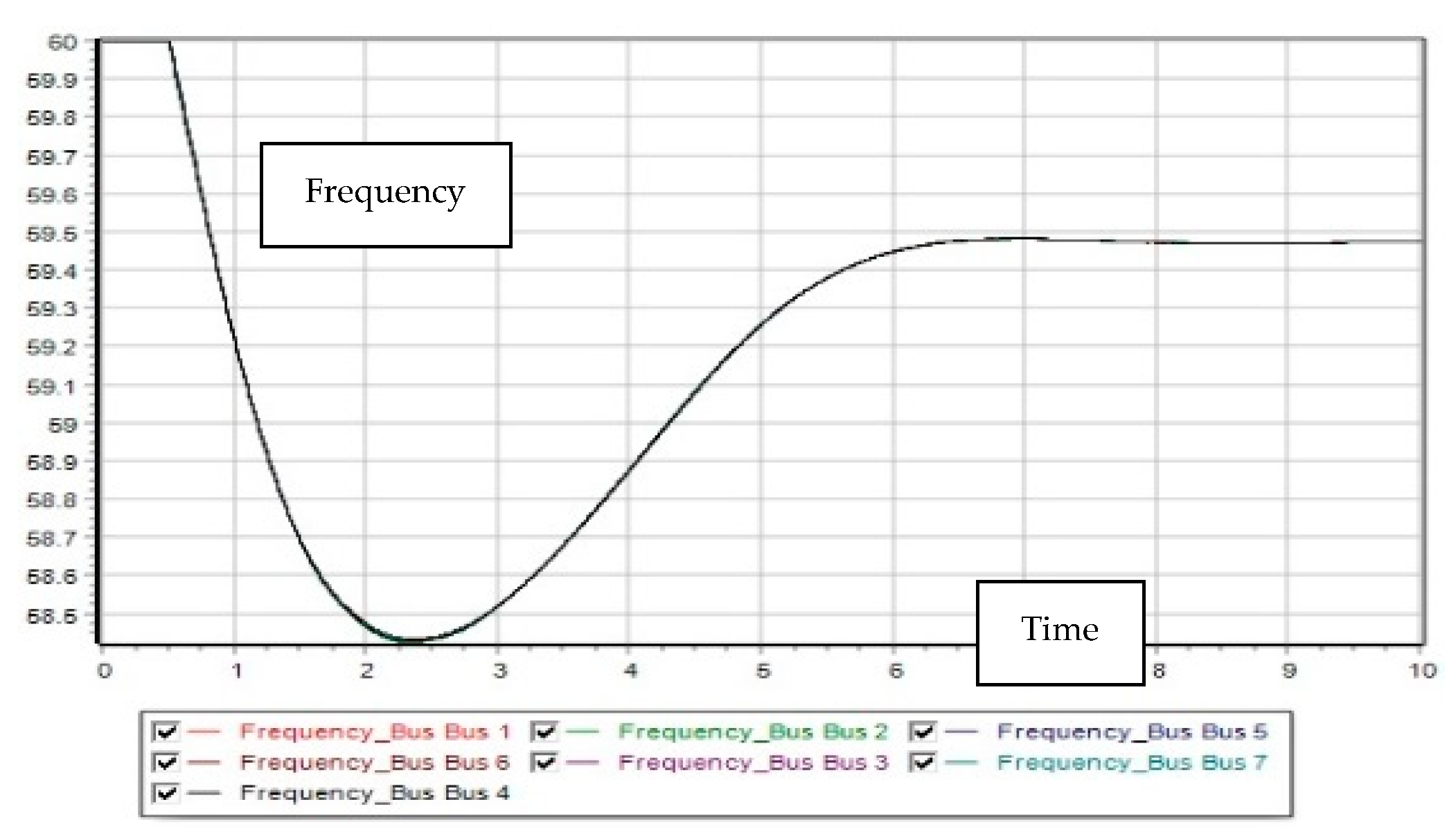
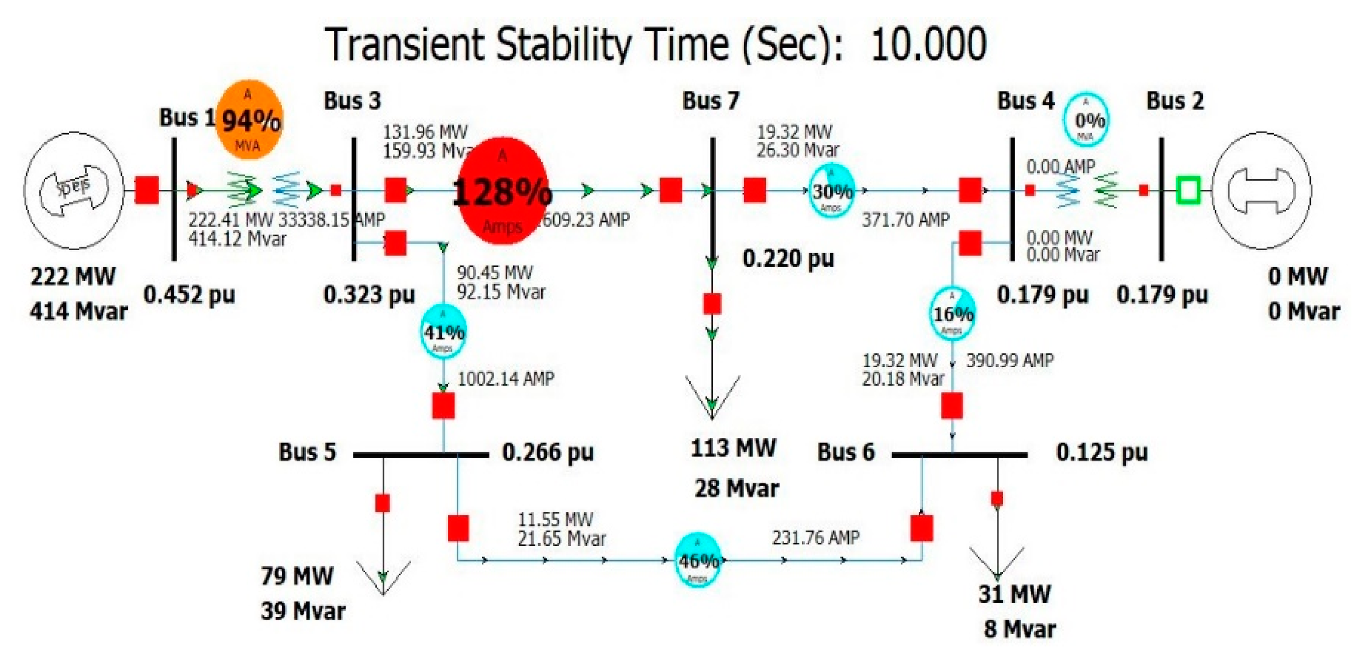
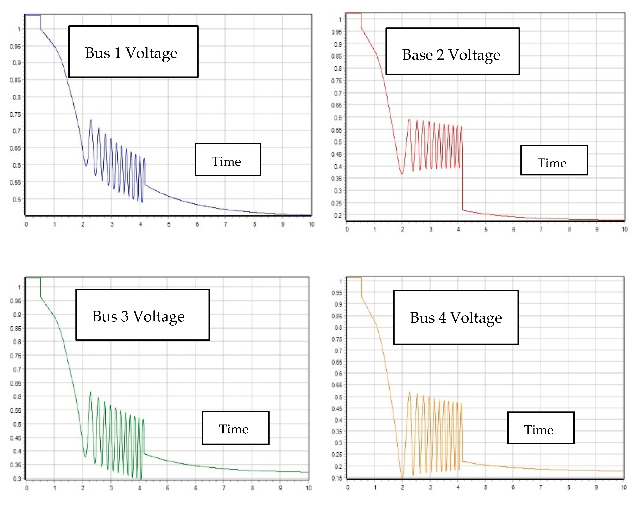
The second contingency scenario is created by 150% increment of load of buses 5 and 7 within 0.5 s. Figure 14 shows the transient stability analysis of the 7-bus system network under the current contingency scenario where the transformer connected to bus 1 is 94% loaded and the generator connected to bus 2 is shut down because the overall load demand becomes more than the maximum generation capacity of 1175 MW and 400 MVar. Therefore, after sudden increment of load at 0.5 s for the second contingency, the slack generator only manages the system load according to its maximum output power. The maximum capacity of the transmission line between bus 3 and 7 is set to 500 MVA, which is already overloaded according to the simulation result. Though the bus frequency is retained at around 60 Hz, the bus voltage drops drastically below 1 pu.
The bus voltages of all buses drop far below 1 pu after 10 s of simulation time. There is a sudden overshoot of bus voltages at around 4.2 s and after that the bus voltages drop drastically, which is shown in Figure 15. Figure 16 shows the variation of rotor angles and generated powers of generators at buses 1 and 2. The rotor angle, generated voltage, and generated power of the generator connected to bus 2 drops far below the steady state value, which is near to zero at 3.6 s, which causes shutdown of that generator. The bus frequency also overshoots at around 4.2 s and increases beyond the steady state system frequency of 60 Hz. After 4.2 s, the bus frequency drops sharply to 60 Hz and retains that until the end of the simulation, which is seen in Figure 17. When the generator at bus 2 shuts down, then the generator connected to the slack bus supplies power to the load of the 7-bus system by keeping the system frequency to 60 Hz. In order to retain the system frequency at 60 Hz, the rotor angle of the slack generator increases after oscillation and gradually cuts down the load of load buses. Though the system becomes unstable, the slack generator supplies power below its maximum generated power to the reduced system load for retaining the system frequency at 60 Hz.
2.2.3. V-Q Sensitivity Analysis
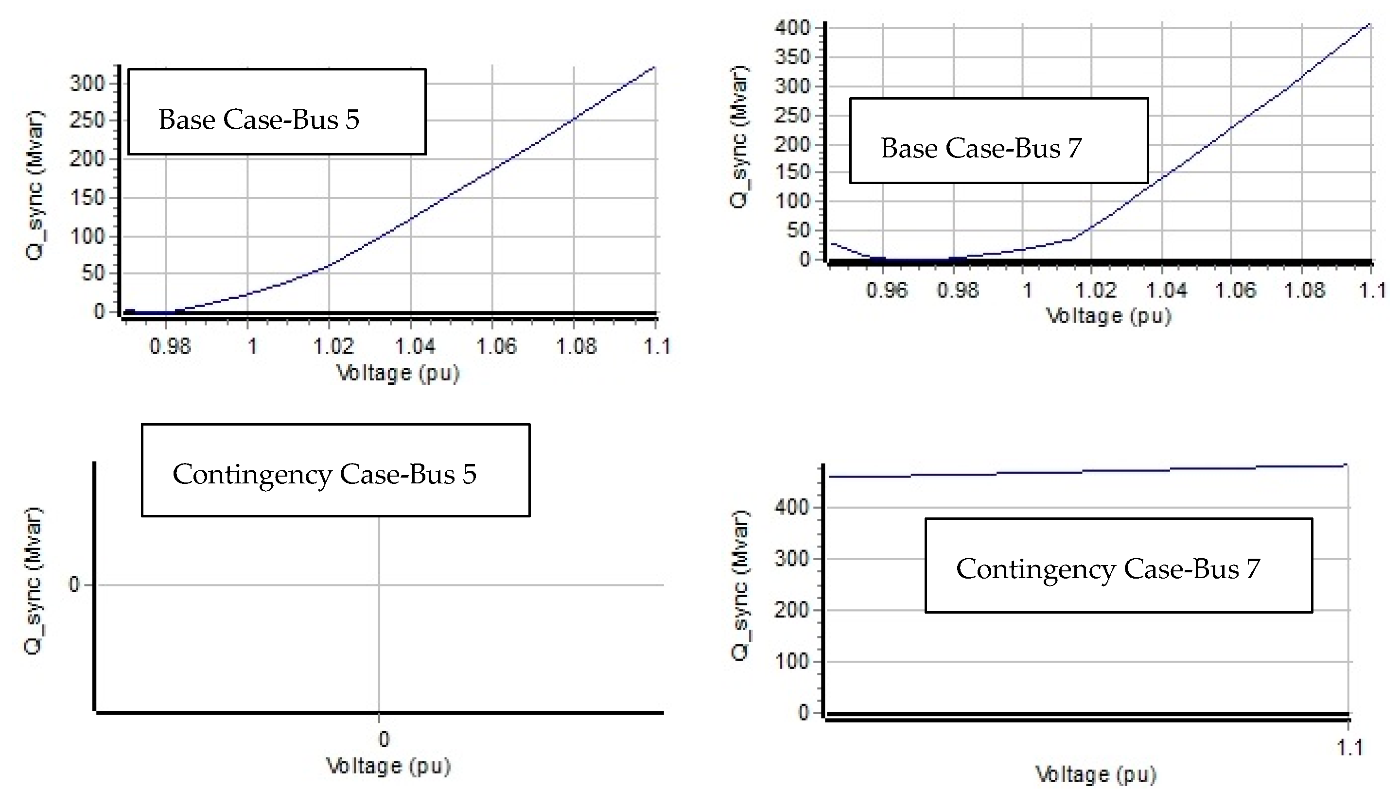
The V-Q sensitivity analysis determines the effect on system voltage due to variation of reactive power of load according to system requirements. If the sensitivity is positive for every bus of any power system, then the system is stable, whereas if the sensitivity is negative for at least one bus, then the system is unstable. Generally, the reactive power voltage (Q-V) curve is plotted either by placing a fictitious generator at the bus which is being analyzed, or by considering the total reactive power injection or absorption at that bus. In case of Q-V curve, the bus voltage and reactive power are represented along x and y axis respectively. The V-Q sensitivity is calculated from the power flow solution at a particular operating point where the slope of the Q-V curve represents the sensitivity at that operating point. Generally, the V-Q sensitivity of load buses of any power system is analyzed according to various contingencies.
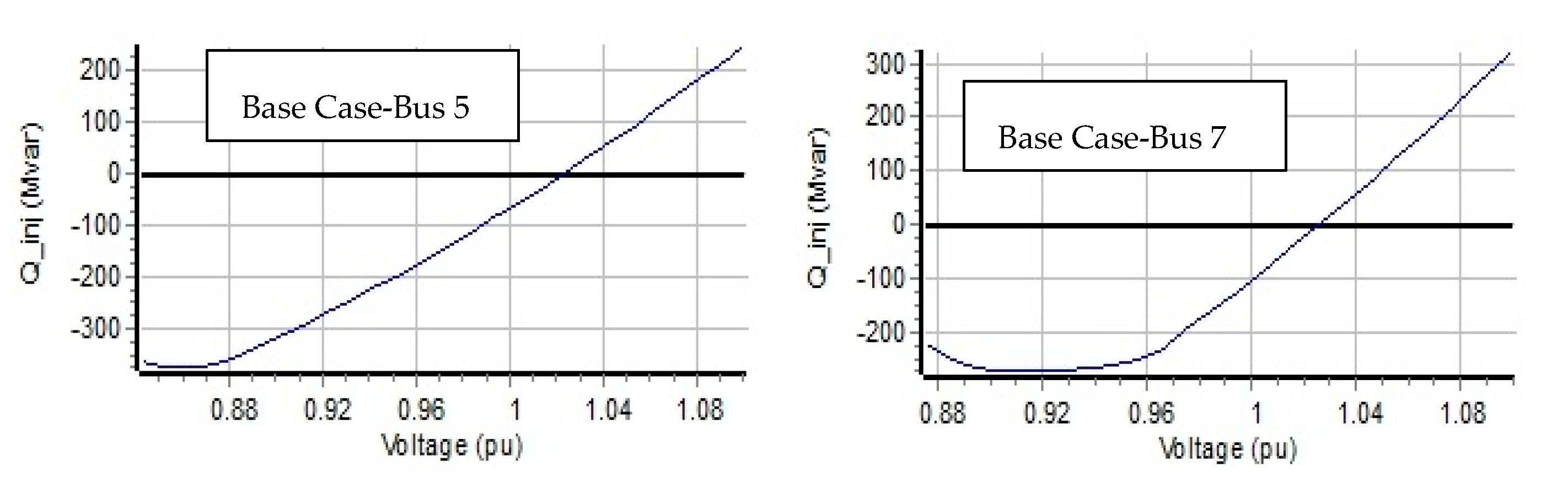
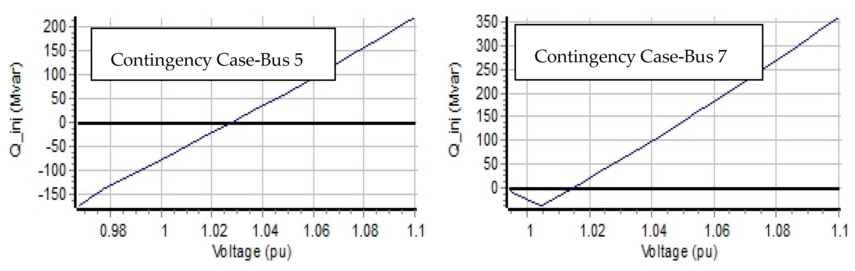
The contingency is created by increasing load at bus 6 to 600 MW and 144 MVar from 400 MW and 100 MVar, respectively, and the load capacity of the transmission line between buses 5 and 6 is reduced to 150 MVA from 200 MVA of the base case. The blackout occurs in the system if the load at bus 6 is increased more than that. Figure 18 shows the base case power flow solution of the simulated model after increment of load at bus 6. The transmission line between buses 5 and 6 is overloaded, and the V-Q sensitivity and Q-V curves of buses 5 and 7 are plotted for the contingency by opening this line. There are two options for plotting Q-V curves by Power World Simulator. In first option, Q is treated as the output of the fictitious synchronous generator, whereas in the second option, Q is treated as the total reactive power injection of the bus. The second option is used for the V-Q sensitivity analysis in this paper. According to Q-V curves of buses 5 and 7, which are shown in Figure 19, the V-Q sensitivity is positive for the base case, which represents the stability of the system though the V-Q sensitivity cannot be determined for the assigned contingency because the Q-V curve does not cross the x axis for bus 7. The Q-V curve of bus 5 cannot be plotted because the power flow does not converge for assigned contingency.
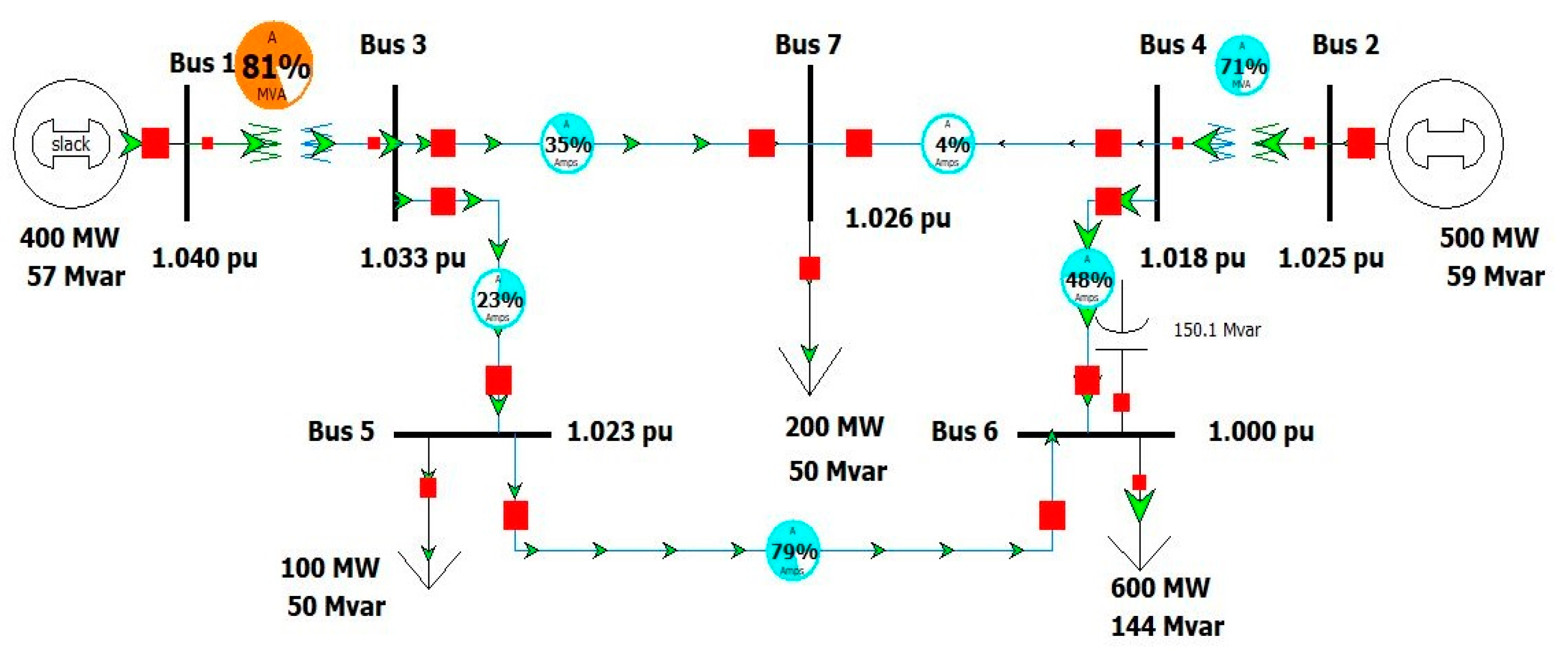
In order to determine V-Q sensitivity of buses 5 and 7 for assigned contingency, a shunt capacitor of nominal value of 150 MVar is connected to bus 6. Figure 20 shows the power flow solution of 7 bus system after adding an additional shunt capacitor to bus 6. Since the shunt capacitor injects additional MVar to the system, the V-Q sensitivity becomes positive for both buses at base and contingency cases. The positive slope of Q-V curves at the assigned contingency represents stability of the 7-bus system after adding the shunt capacitor at bus 6, which is represented in Figure 21.
2.2.4. V-P Sensitivity Analysis
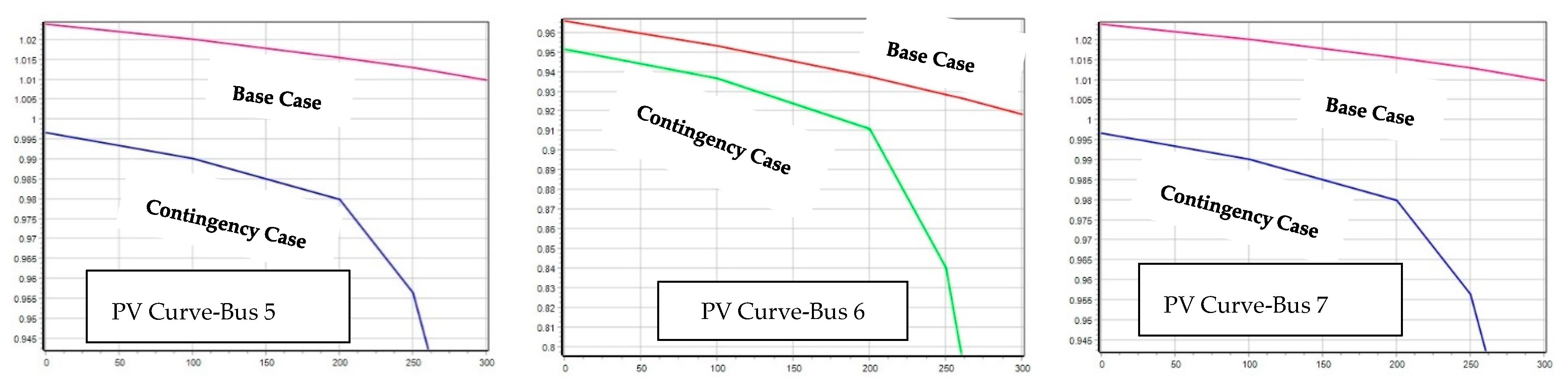
The voltage stability is the ability of a power system to maintain acceptable voltage at all buses under normal operating condition as well as different contingencies. If the voltage stability is hampered due to a local voltage collapse, then that may cause widespread collapse of the overall power system. The V-P sensitivity is an indicator of voltage stability and for that a series of power flow solutions are conducted for monitoring impact on system voltage. The relationship of voltage to power transfer is nonlinear, and therefore a series of power flow solutions is required for retaining constant system voltage for specific buses. The real power voltage (P-V) curves are plotted for each bus for determining the V-P sensitivity according to assigned injection groups. The injection groups are defined according to region or segment of any power system which exports and imports power according to the system requirement. The groups act in unison for transferring power throughout the electricity network, which are classified as source and sink. Generally, at the knee of the P-V curve, voltage drops rapidly with an increase in real power transfer and the power flow solution fails to converge beyond this limit, which is an indication of instability. The contingency scenario is created by 100% increment of load at buses 5 and 7 for V-P sensitivity analysis. Figure 22 shows the final power flow result after several power flow solutions for balancing power transfer according to selected injection groups and contingency. The generators at buses 1 and 2 are selected as a source injection group while load buses of 5, 6, and 7 are selected as load injection group. The P-V curves are plotted for all load buses where the variation of bus voltages in pu is represented with respect to shift of real power (in MW). According to the simulation result, the maximum shift of real power is 260 MW and the mismatch of real and reactive powers are around 1.49 MW and 3.68 Mvar, respectively, for buses 2 and 6 for assigned contingency which cannot be resolved by power flow solution. The P-V curves of buses 5, 6, and 7 are represented in Figure 23 where the nose point of the curves is attained at 260 MW for assigned contingency, and after the nose point the bus voltages drop drastically, which represents an unstable system. The positive section before the nose point is plotted in the curves where the V-Q sensitivity is high near the nose point. For the base case, the P-V curves are mostly flat for three buses which represents a stable system.
3. Discussion
To replicate the impacts on system stability due to uncoordinated fast charging of electric ferries, a simulated model of grid interactive marine battery charging system is analyzed in this paper. According to the simulation result, the uncoordinated fast charging BESS consumes a significant amount of current in a short time in comparison to that of slow charging, which is analogous to a sudden increment of load in the power system. The probable impacts of uncoordinated fast charging on system stability are a sudden change in system voltage and frequency. The voltage unbalance factor and THD are analyzed for sudden increment of load by an IEEE 5 bus system. For identifying the impacts of sudden load increment, three cases are considered by increasing 25%, 50%, and 75% of base load, respectively. According to load flow analysis, the voltage unbalance factors are 0.01% and 200% for all buses at fundamental frequency and third harmonics frequency, respectively, while bus voltages of some buses drop below 1 per unit with load increment. The THD at fundamental frequency for actual 5 bus system is 0.16%, while for three selected cases that becomes 0.16%, 0.16%, and 0.18%, respectively, which represents voltage distortion at high frequency. The transient stability, V-Q, and V-P sensitivity analysis are done for a 7-bus power system by using Power World Simulator. Two contingency scenarios are created by 100% and 150% load increment with respect to base case for two load buses in order to create a situation of sudden load increment in power grid due to uncoordinated fast charging. According to the simulation results, all bus voltages except slack bus are dropped to their steady state value, and all bus frequencies reach near to the system frequency of 60 Hz after continuous fluctuation within the simulation time period for the first contingency. The rotor angles of generators start to oscillate with sudden increase in load and then reach to an equilibrium point for maintaining system stability. The rotor angles vary in accordance with the generated powers, which validate the swing equation of the synchronous machine.
The 7-bus system becomes unstable for the second contingency case and all bus voltages drop drastically below 1 pu, though the system frequency retains at 60 Hz after initial overshoot. The system instability forces to shut down the generator connected to bus 2 with sudden decrease of corresponding rotor angle, generated voltage, and power to zero. In order to retain the system frequency at 60 Hz, the slack generator supplies power to the reduced load by increasing its rotor angle after oscillation. The V-Q sensitivity analysis is performed for load buses 5 and 7 by opening overloaded line between buses 5 and 6, increasing load in bus 6, and reducing the load capacity of the transmission line between buses 5 and 6. Due to non-converge of power flow analysis, the Q-V curve cannot be plotted for bus 5 for the assigned contingency, which is solved by adding a shunt capacitor at bus 6. The positive V-Q sensitivity of buses 5 and 7 represents system stability and V-Q sensitivity for other load buses can also be analyzed for similar contingency. The V-P sensitivity analysis is performed by 100% increment of load at buses 5 and 7 with selected injection groups. The simulation results show that power is shared and shifted among load buses with maximum shift of power is 260 MW and mismatch of real and reactive powers are around 1.49 MW and 3.68 Mvar for buses 2 and 6, respectively. The P-V curves of buses 5, 6, and 7 attain nose point at 260 MW, and the V-Q sensitivity is high near the nose point, and after the nose point the bus voltages drop sharply for the assigned contingency which represents system instability.
The procedure which is used in this paper for determining the impacts of sudden load increment for a simple electricity network is analogous to the inclusion of uncoordinated fast charging load of EF to grid in G2F mode. The similar procedure may be used for identifying similar impacts on a complex power system network with a large number of buses. However, for better understanding the impacts of fast charging of EF on power system, coordinated charging in G2F mode needs to be analyzed along with the actual load characteristics of fast charging. Moreover, F2G operation needs to be investigated for restoring power system stability and supporting ancillary services for integrating of green electricity to grid. The charging and discharging characteristics along with degradation of the battery can be considered for finding actual impacts on grid. The real time simulator, which can interact with the real power system, may give better results on analyzing impacts of fast charging of EF on local grid. A realistic analysis can only be attained when power system stability parameters are defined according to actual data from a power system. In future work, we will investigate the coordinated charging for G2F approach along with F2G application in discharging mode. The battery degradation with charging and discharging characteristics will be analyzed for identifying its impact on electricity network. The application of different control topology for restoring system stability will also be discussed in future work.
Author Contributions
Conceptualization and methodology, R.B.R. and S.A.; prepared the software based simulated model and simulation results, R.B.R.; justification, visualization, and formal analysis of simulated results, R.B.R., S.A., and S.J.A.; draft preparation, review and editing of the paper, R.B.R., S.A., and S.J.A. All authors have read and agreed to the published version of the manuscript.
Funding
This research received no external funding.
Institutional Review Board Statement
Not applicable.
Informed Consent Statement
Not applicable.
Data Availability Statement
The data presented in this study are available on request from the corresponding author. The data are not publicly available because the research findings will be utilized in our future research project.
Conflicts of Interest
The authors declare no conflict of interest.
Abbreviations
| A | Ampere |
| AC | Alternating Current |
| BESS | Battery Energy Storage System |
| CC | Constant Current |
| CV | Constant Voltage |
| CC-CV | Constant current Constant voltage |
| DC | Direct Current |
| EF | Electric Fleet |
| EV | Electric Vehicle |
| FFT | Fast Fourier Transform |
| F2G | Ferry to Grid |
| G2F | Grid to Ferry |
| GHG | Greenhouse Gas |
| Hz | Hertz |
| IMO | International Maritime Organization |
| kW | Kilo Watt |
| kV | Kilo Volt |
| MJ/km | Megajoule per Kilometer |
| MVA | Mega Volt Ampere |
| MW | Mega Watt |
| Mvar | Mega Var |
| PQ | Real Power Reactive Power |
| P-V | Real power Voltage |
| pu | Per Unit |
| PV | Photovoltaic |
| Q | Reactive Power |
| Q-V | Reactive Power Voltage |
| V | Volt |
| V2G | Vehicle to Grid |
| V-P | Voltage Real Power |
| V-Q | Voltage Reactive Power |
| SOC | State of Charging |
| THD | Total Harmonic Distortion |
References
- IEA. World Energy Statistics 2017; OECD Publishing: Paris, France, 2017. [Google Scholar]
- Smith, T.W.P.; Jalkanen, J.P.; Anderson, B.A.; Corbett, J.J.; Faber, J.; Hanayama, S.; O’Keeffe, E.; Parker, S.; Johansson, L.; Aldous, L.; et al. Third IMO GHG Study 2014; International Maritime Organization: London, UK; Micropress Printers: Suffolk, UK, 2015. [Google Scholar]
- Buhaug, Ø.; Corbett, J.J.; Endresen, Ø.; Eyring, V.; Faber, J.; Hanayama, S.; Lee, D.S.; Lee, D.; Lindstad, H.; Markowska, A.Z.; et al. Second IMO GHG Study 2009; International Maritime Organization: London, UK; CPI Books Limited: Reading, UK, 2009. [Google Scholar]
- Zavoda, F.; Puertas, R.R.; Dupre, J.L. Impacts of fast charging stations on grid quality. In Proceedings of the 25th International Conference on Electricity Distribution, CIRED, Madrid, Spain, 3–6 June 2019. [Google Scholar]
- Chandrasekaran, R. Quantification of bottlenecks to fast charging of lithium ion-insertion cells for electric vehicles. J. Power Sources 2014, 271, 622–632. [Google Scholar] [CrossRef]
- Ghavami, A.; Kar, K.; Gupta, A. Decentralized Charging of Plug-in Electric Vehicles with Distribution Feeder Overload Control. IEEE Trans. Autom. Control 2016, 61, 3527–3532. [Google Scholar] [CrossRef]
- Skugor, B.; Deur, J. A novel model of electric vehicle fleet aggregate battery for energy planning studies. Energy 2015, 92, 444–455. [Google Scholar] [CrossRef]
- Xu, Z.; Su, W.; Hu, Z.; Song, Y.; Zhang, H. A hierarchical framework for coordinated charging of plug-in electric vehicles in China. IEEE Trans. Smart Grid 2016, 7, 428–438. [Google Scholar] [CrossRef]
- Lund, H.; Østergaard, P.A.; Connolly, D.; Ridjan, I.; Mathiesen, B.V.; Hvelplund, F.; Thellufsen, J.Z.; Sorknæs, P. Energy storage and smart energy systems. Int. J. Sustain. Energy Plan. Manag. March 2016, 11, 3–14. [Google Scholar]
- Kempton, W.; Tomic, J. Vehicle-to-Grid Power Implementation: From Stabilizing the Grid to Supporting Largescale Renewable Energy. J. Power Sources 2005, 144, 268–279. [Google Scholar] [CrossRef]
- Ma, Y.; Houghton, T.; Cruden, A.; Infield, D. Modeling the benefits of vehicle-togrid technology to a power system. IEEE Trans. Power Syst. 2012, 27, 1012–1020. [Google Scholar] [CrossRef]
- Skugor, B.; Deur, J. A techno-economic analysis of an isolated energy system including electric delivery vehicle fleet and renewable energy sources. In Proceedings of the 10th Conference on Sustainable Development of Energy, Water and Environment Systems (SDEWES), Dubrovnik, Croatia, 27 September–2 October 2015. [Google Scholar]
- Habib, S.; Kamran, M.; Rashid, U. Impact analysis of vehicle to grid technology and charging strategies of electric vehicles on distribution networks—A review. J. Power Sources 2015, 277, 205–214. [Google Scholar] [CrossRef]
- Yifeng, H.; Venkatesh, B.; Guan, L. Optimal scheduling for charging and discharging of electric vehicles. IEEE Trans. Smart Grid 2012, 3, 1095–1105. [Google Scholar]
- Parks, K.; Denholm, P.; Markel, T. Costs and Emissions Associated with Plug-In Hybrid Electric Vehicle Charging in the Xcel Energy Colorado Service Territory; Tech. Rep. NREL/TP-640-41410; National Renewable Energy Laboratory: Boulder, CA, USA, 2007. [Google Scholar]
- Schuller, A.; Ilg, J.; Van Dinther, C. Benchmarking Electric Vehicle Charging Control Strategies. In Proceedings of the 2012 IEEE PES Innovative Smart Grid Technologies (ISGT), Berlin, Germany, 14–17 October 2012. [Google Scholar]
- Aziz, M.; Oda, T.; Ito, M. Battery Assisted Charging System for Simultaneous Charging of Electric Vehicles. Energy 2016, 100, 82–90. [Google Scholar] [CrossRef]
- Paul, S.; Padhy, N.P. Resilient scheduling portfolio of residential device sand plug-in electric vehicle by minimizing conditional value at risk. IEEE Trans. Ind. Inf. 2019, 15, 1566–1578. [Google Scholar] [CrossRef]
- Scarabaggio, P.; Carli, R.; Cavone, G.; Dotoli, M. Smart Control Strategies for Primary Frequency Regulation through Electric Vehicles: A Battery Degradation Perspective. Energies 2020, 13, 4586. [Google Scholar] [CrossRef]
- Lund, H.; Werner, S.; Wiltshire, R.; Svendsen, S.; Thorsen, J.E.; Hvelplund, F.; Mathiesen, B.V. 4th Generation District Heating (4GDH): Integrating smart thermal grids into future sustainable energy systems. Energy 2014, 68, 1–11. [Google Scholar] [CrossRef]
- Carli, R.; Dotoli, M.; Jantzen, J.; Kristensen, M.; Othman, B.S. Energy Scheduling of a Smart Microgrid with shared Photovoltaic Panels and Storage: The case of the Bllen Marina in Samsø. Energy 2020, 198, 117188. [Google Scholar] [CrossRef]
- Zhang, C.; Chen, C.; Sun, J.; Zheng, P.; Lin, X.; Bo, Z. Impacts of electric vehicles on the transient voltage stability of distribution network and the study of improvement measures. In Proceedings of the 2014 IEEE PES Asia-Pacific Power and Energy Engineering Conference (APPEEC), Hong Kong, China, 7–10 December 2014; pp. 1–6. [Google Scholar]
- Dharmakeerthi, C.H.; Mithulananthan, N.; Saha, T.K. Impact of electric vehicle fast charging on power system voltage stability. Int. J. Electr. Power Energy Syst. 2014, 57, 241–249. [Google Scholar] [CrossRef]
- Dharmakeerthi, C.H.; Mithulananthan, N.; Saha, T.K. Overview of the impacts of plug-in electric vehicles on the power grid. In Proceedings of the Innovative Smart Grid Technologies (ISGT) Asia Conference, Perth, Australia, 13–16 November 2011. [Google Scholar]
- Clement-Nyns, K.; Haesen, E.; Driesen, J. The impact of charging plug-in hybrid electric vehicles on a residential distribution grid. IEEE Trans. Power Syst. 2010, 25, 371–380. [Google Scholar] [CrossRef] [Green Version]
- Maheshwari, A.; Paterakis, N.G.; Santarelli, M.; Gibescu, M. Optimizing the operation of energy storage using non-linear lithium-ion battery degradation model. Appl. Energy 2020, 261, 114360. [Google Scholar] [CrossRef]
- Pillay, P.; Manyage, M. Definitions of voltage unbalance. IEEE Power Eng. Rev. 2001, 5, 50–51. [Google Scholar] [CrossRef]
Figure 1.
Simulated model of a grid connected battery charging system.

Figure 2.
Battery current, voltage, state of charging and temperature in case of slow charging.


Figure 3.
Battery current, voltage, SOC, and temperature in case of fast charging.

Figure 4.
Generated voltage and current of alternator.

Figure 5.
Generated voltage and current of solar photovoltaic (PV) system.

Figure 6.
Single line diagram of the 5 bus IEEE network.

Figure 7.
Simulated model of the IEEE 5 bus system.

Figure 8.
FFT (Fast Fourier Transform) analysis of the actual bus system and first two cases.

Figure 9.
Base case power flow solution of the 7 bus power system network.

Figure 10.
Transient stability power flow solution for first contingency scenario.

Figure 11.
Fluctuation of bus voltage due to sudden increment of load at buses 5 and 7.

Figure 12.
Rotor angle and generated power of generators connected to buses 1 and 2.

Figure 13.
Fluctuation of bus frequency due to sudden increment of load at buses 5 and 7.

Figure 14.
Transient stability power flow solution for the second contingency scenario.

Figure 15.
Bus voltages for second transient contingency scenario.


Figure 16.
Rotor angle and generated power of generators of buses 1 and 2.

Figure 17.
Bus frequency for second transient contingency scenario.


Figure 18.
Power flow of 7 bus system after load increment at bus 6.

Figure 19.
Q-V (Reactive Power Voltage) curves of buses 5 and 7.

Figure 20.
Power flow of the 7 bus system after adding a shunt capacitor to bus 6.

Figure 21.
Q-V curves of buses 5 and 7 after adding a shunt capacitor to bus 6.


Figure 22.
Final power flow scenario according to assigned injection group and contingency.

Figure 23.
P-V curves of buses 5, 6, and 7.


Table 1.
Load flow results of the IEEE 5 bus system.
| Bus No. | Generation | Load Demand | Bus Voltage | Total Generation | Total Load | |||||
|---|---|---|---|---|---|---|---|---|---|---|
| No. | MW | Mvar | MW | Mvar | Voltage (pu) | Angle (degree) | MW | Mvar | MW | Mvar |
| 1 | 129.59 | −7.42 | 0 | 0 | 1.06 | 0 | 169.59 | 22.58 | 165 | 40 |
| 2 | 40 | 30 | 20 | 10 | 1.0474 | −2.8063 | ||||
| 3 | 0 | 0 | 45 | 15 | 1.0242 | −4.997 | ||||
| 4 | 0 | 0 | 40 | 5 | 1.0236 | −5.3291 | ||||
| 5 | 0 | 0 | 60 | 10 | 1.0179 | −6.1503 | ||||
Table 2.
Load flow results of the IEEE 5 bus system of case 1.
| Bus No. | Generation | Load Demand | Bus Voltage | Total Generation | Total Load | |||||
|---|---|---|---|---|---|---|---|---|---|---|
| No. | MW | Mvar | MW | Mvar | Voltage (pu) | Angle (degree) | MW | Mvar | MW | Mvar |
| 1 | 173.87 | 12.50 | 0 | 0 | 1.06 | 0 | 213.87 | 42.50 | 206 | 50 |
| 2 | 40 | 30 | 30 | 12.5 | 1.0341 | −3.71 | ||||
| 3 | 0 | 0 | 55 | 17.5 | 1.0049 | −6.41 | ||||
| 4 | 0 | 0 | 51.26 | 7.5 | 1.0032 | −6.84 | ||||
| 5 | 0 | 0 | 70 | 12.5 | 0.9965 | −7.75 | ||||
Table 3.
Load flow results of the IEEE 5 bus system of case 2.
| Bus No. | Generation | Load Demand | Bus Voltage | Total Generation | Total Load | |||||
|---|---|---|---|---|---|---|---|---|---|---|
| No. | MW | Mvar | MW | Mvar | Voltage (pu) | Angle (degree) | MW | Mvar | MW | Mvar |
| 1 | 219.20 | 35.67 | 0 | 0 | 1.06 | 0 | 259.20 | 65.67 | 247.5 | 60 |
| 2 | 40 | 30 | 40 | 15 | 1.0196 | −4.64 | ||||
| 3 | 0 | 0 | 65 | 20 | 0.9839 | −7.88 | ||||
| 4 | 0 | 0 | 62.5 | 10 | 0.9811 | −8.44 | ||||
| 5 | 0 | 0 | 80 | 15 | 0.9732 | −9.44 | ||||
Table 4.
Load flow results of the IEEE 5 bus system of case 3.
| Bus No. | Generation | Load Demand | Bus Voltage | Total Generation | Total Load | |||||
|---|---|---|---|---|---|---|---|---|---|---|
| No. | MW | Mvar | MW | Mvar | Voltage (pu) | Angle (degree) | MW | Mvar | MW | Mvar |
| 1 | 265.79 | 62.66 | 0 | 0 | 1.06 | 0 | 305.79 | 92.66 | 288.75 | 70 |
| 2 | 40 | 30 | 50 | 17.5 | 1.0037 | −5.60 | ||||
| 3 | 0 | 0 | 75 | 22.5 | 0.9610 | −9.45 | ||||
| 4 | 0 | 0 | 73.75 | 12.5 | 0.9569 | −10.13 | ||||
| 5 | 0 | 0 | 90 | 17.5 | 0.9477 | −11.25 | ||||
Table 5.
Allowable total harmonic distortion (THD) value according to the IEEE 519-2014 standard.
| Bus Voltage, V | Total Harmonic Distortion |
|---|---|
| V <= 10 kV | 8% |
| 10 kV < V <= 69 kV | 5% |
| 69 kV < V <= 161 kV | 2.5% |
| 161 kV < V | 1.5% |
Publisher’s Note: MDPI stays neutral with regard to jurisdictional claims in published maps and institutional affiliations. |
© 2021 by the authors. Licensee MDPI, Basel, Switzerland. This article is an open access article distributed under the terms and conditions of the Creative Commons Attribution (CC BY) license (http://creativecommons.org/licenses/by/4.0/).
Share and Cite
MDPI and ACS Style
Roy, R.B.; Alahakoon, S.; Arachchillage, S.J. Grid Impacts of Uncoordinated Fast Charging of Electric Ferry. Batteries 2021, 7, 13. https://0-doi-org.brum.beds.ac.uk/10.3390/batteries7010013
AMA Style
Roy RB, Alahakoon S, Arachchillage SJ. Grid Impacts of Uncoordinated Fast Charging of Electric Ferry. Batteries. 2021; 7(1):13. https://0-doi-org.brum.beds.ac.uk/10.3390/batteries7010013
Chicago/Turabian StyleRoy, Rajib Baran, Sanath Alahakoon, and Shantha Jayasinghe Arachchillage. 2021. "Grid Impacts of Uncoordinated Fast Charging of Electric Ferry" Batteries 7, no. 1: 13. https://0-doi-org.brum.beds.ac.uk/10.3390/batteries7010013
Note that from the first issue of 2016, this journal uses article numbers instead of page numbers. See further details here.