Combining the Distribution of Relaxation Times from EIS and Time-Domain Data for Parameterizing Equivalent Circuit Models of Lithium-Ion Batteries

Abstract

Equivalent circuit models (ECMs) are a widely used modeling approach for lithium-ion batteries in engineering applications. The RC elements, which display the dynamic loss processes of the cell, are usually parameterized by fitting the ECM to experimental data in either the time-domain or the frequency-domain. However, both types of data have limitations with regard to the observable time constants of electrochemical processes. This work proposes a method to combine time-domain and frequency-domain measurement data for parameterization of RC elements by exploiting the full potential of the distribution of relaxation times (DRT). Instead of using only partial information from the DRT to supplement a conventional fitting algorithm, we determine the parameters of an arbitrary number of RC elements directly from the DRT. The difficulties of automated deconvolution of the DRT, including regularization and the choice of an optimal regularization factor, is tackled by using the L-curve criterion for optimized calculation of the DRT via Tikhonov regularization. Three different approaches to merge time- and frequency-domain data are presented, including a novel approach where the DRT is simultaneously calculated from electrochemical impedance spectoscropy (EIS) and pulse relaxation measurements. The parameterized model for a commercial 18650 NCA cell was validated during a validation cycle consisting of constant current and real-world automotive cycling and yields a relative improvement of over 40% compared to a conventional EIS-fitting algorithm.

1. Introduction

1.1. Motivation

In recent years, lithium-ion batteries (LIBs) have become ubiquitous in many applications. Their advantages in terms of power and energy density over other storage mediums make them the most promising candidate for electric mobility and stationary energy storage. To optimize the operation of lithium-ion batteries, the estimation of battery states such as the state of charge (SOC), state of health (SOH), and state of available power (SOAP) is required.

To estimate the different states of lithium-ion batteries, battery management systems (BMSs) typically employ battery models, which are parameterized in order to best reproduce the electrochemical behavior of the battery. The battery states are then either estimated directly from model parameters, such as from the impedance parameters for the SOAP, or by comparing the measured voltage and model voltage to estimate the SOC and SOH with subsequent algorithms, such as a Kalman filter [1].

To keep the computational effort low to ensure real-time capability and to ensure convergence of estimation algorithms, the complexity of such models and algorithms has to be limited. A widespread type of model used for this purpose is the equivalent circuit model (ECM), the complexity of which can easily be adjusted by the number of its circuit elements and the parameterization of which does not require destructive analysis of the cell’s geometry and material properties. The idea behind ECMs is to model the lithium-ion battery (LIB) with standard circuit elements such as an ideal voltage source modeling the open-circuit behavior, and resistors and capacitors, modeling the kinetics of the LIB. The key challenge lies in parameterization of these circuit elements to ensure high accuracy of BMS algorithms. Thereby, the characterization of the kinetics especially, expressed by the lithium-ion batteries impedance, is of great importance, since a limited set of parameters must cover a broad range of different dynamics in the load profile.

Furthermore, lithium-ion batteries degrade over their lifetime, which, besides capacity fade, also leads to an increase of the impedance [2]. However, the aging trajectory of an individual LIB is highly dependent on the operating conditions such as temperature, voltage window, and current [3,4]. This demands on-line algorithms, which are able to continuously track the battery impedance parameters to keep the ECM up to date [5]. The accuracy of such on-line optimization algorithms often depends on suitable initial values [6]. Hence, accurate estimation of impedance parameters under laboratory conditions, before deployment of the LIB, is needed.

1.2. State of the Art

Many different approaches for estimating the parameters of the circuit elements in ECMs can be found in the literature [7,8,9]. There are two types of measurements which are usually employed for impedance characterization of LIB: electrochemical impedance spectoscropy (EIS) in the frequency-domain and measurements in the time-domain, e.g., current pulses. The most crucial difference between both methods is the frequency range of electrochemical processes that can be reliably investigated with them. EIS, on the one hand, is very reliable in the high-frequency region up to a few $\mathrm{M}\mathrm{Hz}$ [10]. However, due to the long charging and discharging phases in the sinusoidal excitation at low frequencies, significant SOC-changes occur, which at some point violate the prerequisite of a linear, time-invariant and causal system [11]. This limits EIS to frequencies above approximately 1 $\mathrm{m}\mathrm{Hz}$ [12]. Time-domain measurements (TDMs), on the other hand, are better suited to investigate the low-frequency behavior, while being limited by the sampling rate and measurement accuracy in the high-frequency region [6].

The impedance spectrum of lithium-ion batteries is usually presented in a Nyquist plot, where, to some extent, the loss processes of the measured system can be made visible. However, the time constants of the different electrochemical processes are often close to each other and cannot be fully separated in the Nyquist plot [13,14]. To isolate the individual processes, the distribution of relaxation times (DRT) of an impedance spectrum can be evaluated, since it provides a higher frequency resolution of the dynamic processes. It shows the distribution of the total polarization resistance in the continuous space of relaxation times. The DRT can be used to identify and separate dynamic processes and to investigate how those processes are affected by operating conditions like temperature or battery states such as SOC and SOH [7,13,15,16,17,18].

A combination use of EIS and TDM is advisable if the electrochemical behavior of a cell is to be investigated in a wide frequency range. For this, the useful insights into the cell’s loss processes provided by the DRT can be used during the parameterization process. Previous efforts, combining both measurement methods with varying extent, are summarized in the following.

Illig et al. [13] used EIS measurements for their ECM parameterization. They first modeled the low-frequency behavior, as well as the purely capacitive behavior, with a capacitance and aWarburg-element, the overvoltage of which they then subtracted from the measurement data. From the remaining impedance spectrum they calculateed the DRT and used it to identify the occurring processes and to determine the starting values of the following fitting algorithm. The model was completed by fitting a series of three RC elements, an ohmic resistance and an inductance to the preprocessed impedance spectrum.

Gantenbein et al. [7] have introduced a physically motivated ECM consisting of an ohmic resistance, two RC elements, oneWarburg element, an inductance, and a capacitance in series. These circuit elements model the ohmic and contact loss, interface loss of the anode, interface loss of the cathode and diffusion loss and capacitive behavior, which they have identified by investigating the DRT of the full cell and its indivual electrodes. The high and medium frequency parts of the model were parameterized by conventional EIS-fitting of the resistance and the RC elements. Diffusion and capacitive behavior were then included in the model by a time-domain fitting of the remaining model parameters.

Withenhausen directly determined certain RC parameters from the DRT [12]. He covered some RC elements by frequency-domain measurements; therefore he used an iterative algorithm, in which several single process peaks were fitted to the DRT. The remaining elements were parameterized by a time-domain fit to the measured voltage relaxation after bringing the cell to a defined SOC.

Schmidt et al. [14] identified ECM parameters purely from the DRT. They used EIS measurements and Fourier-transformed time-domain measurements, which were merged into one impedance spectrum. From this spectrum the DRT was calculated. Together with an added ohmic resistance, the discrete DRT then served directly as an ECM, which led to the relaxation times of its RC elements being evenly spaced on a logarithmic scale like the data points of the DRT. They evaluated the impact of the chosen model order on their parameterization procedure by comparing model configurations with 100, 20, 10, and 4 RC elements. Due to the a priori fixed time constants without physical meaning they needed a comparatively high number of RC elements to obtain an adequate model accuracy.

It can be concluded that in the previous literature, the DRT is often only used to gain a priori knowledge on the investigated cell to enhance conventional fitting algorithms, e.g., by a non-linear least squares algorithm, in either the frequency-domain or timedomain. Such fitting algorithms have the disadvantage that they are highly dependent on boundary conditions and initial starting values, which leads to a time-consuming and iterative parameterization process. The DRT, however, contains the full information of the cell’s impedance, which is why we propose an approach to determine RC parameters directly from the DRT.

1.3. Contributions

This work aims to exploit the potential of the DRT during an automated identification of RC parameters of an ECM. The main contributions of our proposed method can be summarized as follows:

• Evaluation of frequency- and time-domain measurements:
  To capture the full dynamic behavior of a cell, both EIS and TDM measurements have been considered in the ECM parameterization process and their DRT computed. Respective measurements in the frequency-domain as well as in the time-domain were performed (Section 2).
• Optimized calculation of the DRT via Tikhonov regularization:
  Since an accurate DRT is essential for the proposed parameterization process, the L-curve criterion was employed to optimize the calculation of the DRT via Tikhonov regularization. Moreover, the impact of different regularization terms on the calculated DRT was investigated (Section 3).
• Process for direct parameterization of RC elements from the DRT:
  Instead of using only partial information from the DRT to supplement a conventional fitting algorithm, the full potential of the DRT was exploited by a parameterization process which determines RC parameters directly from the DRT (Section 4).
• Analysis of various data merging approaches:
  Different methods of combining EIS and TDM data in the parameterization process are presented in this work. One of those methods includes a new way of calculating the DRT using TDM and EIS simultaneously, uniting the steps of DRT calculation and merging frequency- and time-domain data (Section 5).

A conclusion is given in Section 6.

2. Experimental

In this work, all experiments were performed with a commercial 18,650 cell of type US18650VTC5A by Sony/Murata with a nominal capacity of $C_{\mathrm{N}}=2.5\mathrm{A}\mathrm{h}$. The anode active material consists of graphite with a small share of silicon, while the cathode active material is nickel cobalt aluminium oxide (NCA) [19]. All measurements were performed at 20 °C inside a Memmert IPP 110 climate chamber.

2.1. EIS

To capture the high-frequency behavior of the cell, EIS measurements were performed in a frequency range from 5 $\mathrm{k}$$\mathrm{Hz}$ to 10 $\mathrm{m}$$\mathrm{Hz}$ with 10 points per decade. Starting at a fully charged state, impedance spectra were recorded in 10% SOC steps with a relaxation period of 3 $\mathrm{h}$ after discharging to the respective SOC. EIS measurements were carried out using a Gamry Interface 5000 test device applying a hybrid EIS mode. This modified form of galvanostatic EIS continuously adjusts the current such that the desired potential of 10 $\mathrm{m}$$\mathrm{V}$ is maintained. In this way, a linear operation range is ensured.

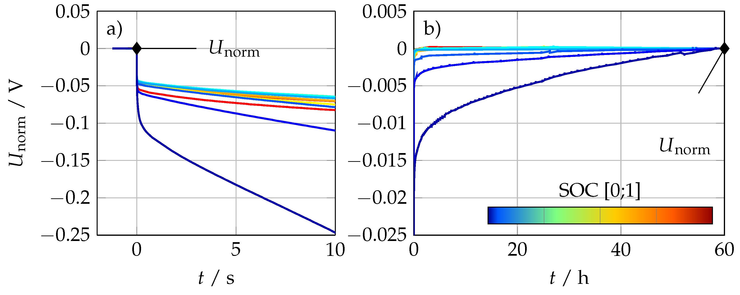
2.2. Time-Domain Measurements (TDMs)

To determine the low-frequency behavior of the cell we performed TDMs. In particular, we applied pulse-relaxation measurements with a discharge pulse current of $I_{\mathrm{p}}=-1C$, a pulse duration of $T_{\mathrm{p}}=10\mathrm{s}$, and a relaxation period of $T_{\mathrm{relax}}=60\mathrm{h}$. To match the EIS, pulse-relaxation measurements were also performed at 11 SOC steps between 100% SOC and 0% SOC. Results are shown in Figure 1.

After bringing a cell to its respective SOC, it is crucial to ensure a fully relaxed state before applying the current pulse. Otherwise, the voltage measurement of the relaxation phase is superimposed by a second relaxation, resulting from the previous SOC change. If this second relaxation results from a previous discharge, it can lead to an overestimated duration of the relaxation process. If this second relaxation results from a previous charge, it can lead to an underestimated duration of the relaxation process or even voltage relaxation in the opposite direction.

Previous researchers observed this behavior and assumed it to be originating from a self-discharge process [20,21]. To isolate the pulse-relaxation behavior, they proposed a preprocessing procedure to remove the self-discharge voltage from the relaxation voltage. We observed that, for the investigated cell, at some SOC relaxation processes were still visible even after two weeks after bringing the cell to its respective SOC. After 3 weeks, however, a constant voltage (within the voltage resolution of the measurement equipment) for longer than $T_{\mathrm{relax}}$ was observed at every tested SOC and pulse measurements could be performed.

In order to reduce the measurement time, a separate pristine cell from the same production batch was used for the pulse-relaxation measurements for each tested SOC step. For all time-domain measurements, the cell test system by the BaSyTec GmbH was used, which records the cell voltage with a resolution of $0.3$ $\mathrm{m}$$\mathrm{V}$ and an accuracy of 1 $\mathrm{m}$$\mathrm{V}$. The first half hour of the measurement was sampled with the maximum sample rate of $0.02$ $\mathrm{s}$. In the further course of the measurement, we reduced the sampling rate to limit the amount of data. The raw measurement data were then logarithmically subsampled to further reduce the number of data points and hence lower computational effort and time, as proposed by Schmidt [20].

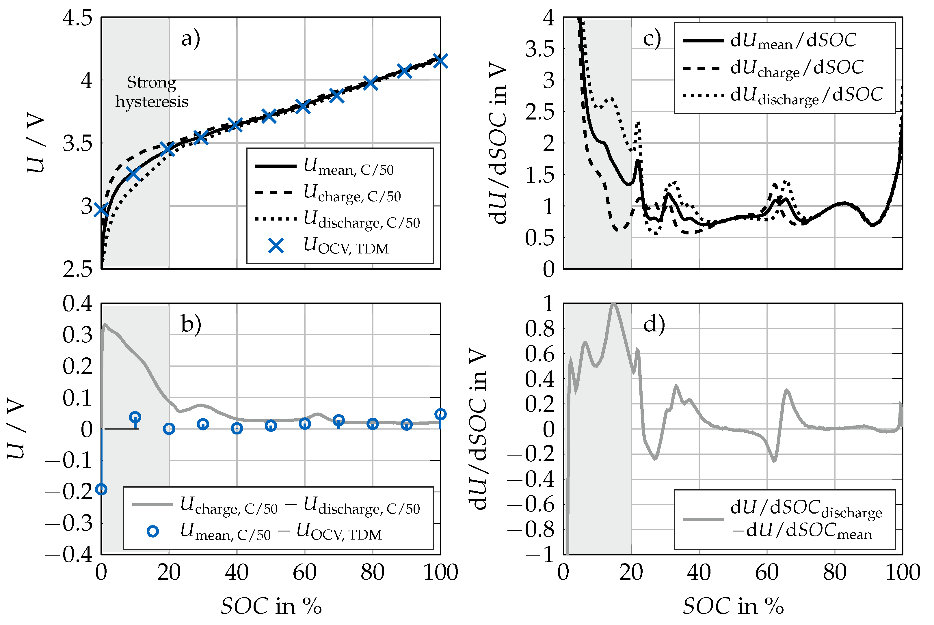
2.3. Open-Circuit Voltage

Besides the dynamic behavior of the cell over a broad frequency range, the cell’s static behavior at thermodynamic equilibrium needs to be characterized to supplement the ECM. This is typically done by the measurement of a pseudo open-circuit voltage (pOCV) with a low current rate or with a galvanostatic intermittent titration technique (GITT), where the open-circuit voltage is measured after bringing the cell to a respective SOC. In Figure 2, the pOCV curve with C/50 is compared to the measured voltage after 3 weeks of relaxation before the pulse-relaxation measurement was performed. Additionally, the differential voltage was analyzed.

It can be seen that the values for $U_{OCV,TDM}$ match well with $U_{mean,C/50}$ for some SOCs. For other SOCs, especially for which the differential voltage analysis (DVA) reveals a greater slope in the voltage curve and also the difference between ${dU/dQ}_{discharge}$ and $dU/dQmean$ increases, $U_{OCV,TDM}$ shows smaller values compared to $U_{mean,C/50}$ (except for 0% SOC, which is mainly due to the measurement procedure of the pOCV). In our study, we validated both OCV determination methods and ultimately chose $U_{OCV,TDM}$, since it is consistent with the pulse-relaxation measurements for the dynamic behavior.

As discussed in [6], the strong divergence between charging and discharging curves in the low SOC area, which is assumed to be caused by the (de-)lithiation competition of graphite and silicon [22], will have a major impact on the validation results, if an averaged pOCV curve or the values for $U_{OCV,TDM}$ are chosen to parameterize the OCV of the ECM. This has to be kept in mind when analyzing the validation results of different configurations of the proposed DRT-fitting (Section 5) and attributing high residuals to either the cell’s thermodynamic or kinetic behavior.

3. Calculation of the DRT

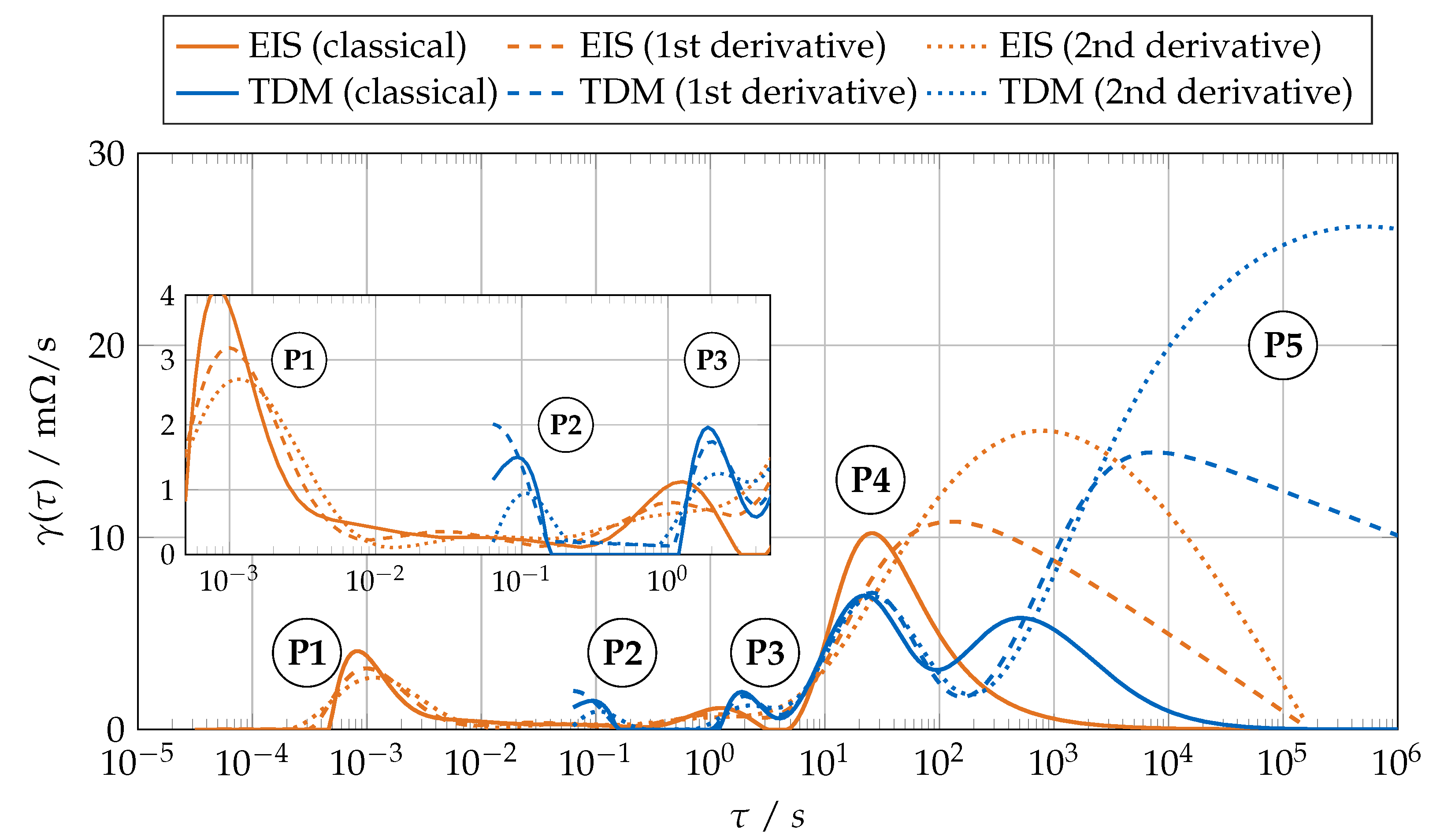
3.1. DRT Calculated from EIS (EIS-DRT)

The DRT is based on the assumption that the impedance of a capacitive electrochemical system can be represented by an infinite number of RC elements with continuous relaxation times [14,23,24]. Based on this assumption, the impedance spectrum of a capacitive electrochemical system can be represented by

$$Z_{\mathrm{DRT}}\left(f\right)={\int }_{-\infty }^{\infty }\frac{\gamma (ln\tau )}{1+j2\pi f\tau }\mathrm{d}ln\tau .$$

(1)

$\gamma (ln\tau )$ can be understood as the distribution of the total polarization resistance along the logarithmic scale of continuous relaxation times $\tau$. Therefore, its integral over the entire space of relaxation times is

$${\int }_{-\infty }^{\infty }\gamma (ln\tau )\mathrm{d}ln\tau =R_{\mathrm{Pol}},$$

(2)

To obtain the DRT from EIS, the difference between $Z_{\mathrm{DRT}}\left(f\right)$ and the experimental data $Z_{\exp }\left(f\right)$ must be minimized by optimization of $\gamma (ln\tau )$. Using matrix notation and a discretized DRT, the optimization goal can be expressed as

$$\underset{R_0,\mathit{R}}{min}∥\left[\begin{array}{cc}\sqrt{w^{\prime }}{\mathit{A}}_{\mathrm{EIS}}^{\prime }& \sqrt{w^{\prime }}\mathbf{1}\\ \sqrt{w^{″}}{\mathit{A}}_{\mathrm{EIS}}^{″}& \mathbf{0}\end{array}\right]\left[\begin{array}{c}\mathit{R}\\ R_0\end{array}\right]-{\left[\begin{array}{c}\sqrt{w^{\prime }}{\mathit{Z}}_{\exp }^{\prime }\\ \sqrt{w^{″}}{\mathit{Z}}_{\exp }^{″}\end{array}\right]∥}_2^2$$

(3)

or short

$$\begin{array}{cccc}\hfill \underset{\mathit{x}}{min}\parallel {\mathit{B}}_{\mathrm{EIS}}& \mathit{x}\hfill & \hfill -& {\mathit{Z}}_{\exp }{\parallel }_2^2.\hfill \end{array}$$

(4)

$\mathit{R}$ is a column vector of the resistances $R_n={\gamma }_n\Delta {\tau }_{\log }$. Since a negative resistance is physically impossible, the additional constraint $x_n\ge 0\forall n$ has to be considered in the problem.

The real part ${\mathit{Z}}^{\prime }$ and the imaginary part ${\mathit{Z}}^{″}$ of the impedance can be taken into account with different weights $w^{ȃ}$ and $w^{″}$ [25]. Due to the Kramers–Kronig relation [26] either one of the two would be adequate for DRT calculation [12,24,27]. However, using both can help to compensate measurement noise. Within this work, both $w^{\prime }$ and $w^{″}$ are set to $0.5$ for an equal weighting. The derivation of Equation (3) as well as the matrices ${\mathit{A}}_{\mathrm{EIS}}^{\prime }$ and ${\mathit{A}}_{\mathrm{EIS}}^{″}$ can be found in Appendix A. The DRT calculated from EIS is referred to as EIS-DRT further on in this paper.

3.2. DRT Calculated from Time-Domain Measurements (TDM-DRT)

Schmidt [20,21] proposes an approach which uses TDM to calculate the DRT. The measurements he uses are conducted in the form of current pulses. To a pulse of magnitude $I_{\mathrm{p}}$ applied at $t_0$ for a duration of $T_{\mathrm{p}}$, a single RC element yields a voltage response of

$$\begin{array}{cc}\hfill u_n(t)=& R_n{I}_{\mathrm{p}}[\sigma (t-t_0)(1-exp(-\frac{t-t_0}{{\tau }_n}))\hfill \\ & -\sigma (t-(t_0+T_{\mathrm{p}}))(1-exp(-\frac{t-(t_0+T_{\mathrm{p}})}{{\tau }_n}))],\hfill \end{array}$$

(5)

with $\sigma \left(x\right)$ being the Heaviside step function. Applying an infinite number of RC elements, i.e., the DRT, yields

$$\begin{array}{cc}\hfill u_{\mathrm{DRT}}\left(t\right)={\int }_{-\infty }^{\infty }& \gamma (ln\tau )I_{\mathrm{p}}[\sigma (t-t_0)(1-exp(-\frac{t-t_0}{\tau }))\hfill \\ & -\sigma (t-(t_0+T_{\mathrm{p}}))(1-exp(-\frac{t-(t_0+T_{\mathrm{p}})}{\tau }))]\mathrm{d}ln\tau .\hfill \end{array}$$

(6)

Analogous to the EIS-DRT, the difference between $u_{\mathrm{DRT}}\left(t\right)$ and the experimental data $u_{\exp }\left(t\right)$ must be minimized by optimization of $\gamma (ln\tau )$. Evaluating the relaxation phase of the pulse measurement, the matrix equation

$$\underset{U_{\mathrm{OCV}},\mathit{R}}{min}\parallel \left[\begin{array}{cc}{\mathit{A}}_{\mathrm{TDM}}& \mathbf{1}\end{array}\right]\left[\begin{array}{c}\mathit{R}\\ {\mathit{U}}_{\mathrm{OCV}}\end{array}\right]-u_{\exp }{\parallel }_2^2$$

(7)

or short

$$\begin{array}{cccc}\hfill \underset{x}{min}\parallel {\mathit{B}}_{\mathrm{TDM}}& \mathit{x}\hfill & \hfill -& {\mathit{u}}_{\exp }{\parallel }_2^2,\hfill \end{array}$$

(8)

can be formed. Again the equation must be minimized while obeying the non-negative constraint $x_n\ge 0\forall n$. As in Equation (3), $\mathit{R}$ is a column vector of the resistances $R_n={\gamma }_n\Delta {\tau }_{\log }$. The derivation of Equation (7) and the matrix $A_{\mathrm{TDM}}$ can be found in Appendix B. The DRT calculated from time-domain data is henceforth referred to as TDM-DRT.

3.3. Tikhonov Regularization

Since the experimental data ${\mathit{Z}}_{\exp }$ and ${\mathit{u}}_{\exp }$ are subject to measurement noise and the number of unknowns does not necessarily fit the number of equations, there is no unique solution to the system of linear equations $\mathit{Bx}={\mathit{D}}_{\exp }$, which makes Equation (3) and Equation (7) ill-posed problems [20,25]. Hence, a mathematical tool for stabilizing the problem and generating a unique solution is required. For this purpose we employ Tikhonov regularization [28]. By adding a regularization term, an additional condition is introduced to the minimization problem, which stabilizes the solution:

$$\underset{x}{min}\left(\parallel \mathit{Bx}-{\mathit{D}}_{\exp }{\parallel }_2^2+\lambda {\parallel \mathit{Lx}\parallel }_2^2\right).$$

(9)

The regularization factor $\lambda$ determines how strong the influence of the regularization term is on the solution. The value of $\lambda$ has to be chosen carefully to achieve accurate results. The matrix $\mathit{L}$ of the regularization term is arbitrary in theory. However, choosing $\mathit{L}$ in a meaningful way allows to penalize specific features of the solution:

• The standard form of the Tikhonov regularization is the regularization with a squared norm of the solution itself. Hence, it penalizes high magnitudes of the solution and therefore favors solutions with smaller peaks. $\mathit{L}$ has to be set to be the identity matrix $\mathit{I}$ such that $\mathit{Lx}=\mathit{x}$ [29].
• The regularization with the squared norm of the solution’s first derivative penalizes high gradients in the solution and therefore favors solutions with moderate slopes. For this, $\mathit{L}$ has to be chosen such that $\mathit{Lx}=\frac{dx}{dln\tau }$, as shown in Appendix C [27,29].
• The regularization with the squared norm of the solution’s second derivative penalizes high curvatures in the solution and therefore favors flat and smooth solutions. For this, $\mathit{L}$ has to be chosen such that $\mathit{Lx}=\frac{d^{2}x}{d{(ln\tau )}^2}$, as shown in Appendix C [20,21,25,29].

The suitability of different regularization terms depends on the shape of the actual DRT, which, however, is not known in most cases. As shown in Figure 3, the choice of the regularization term has a major impact on the solution. Still, the revealed processes are consistent for EIS-DRT (four identified processes P1–P4) and TDM-DRT (four identified processes P2–P5).

The regularization with the solution’s second derivative yields wide peaks, especially in the low-frequency range. The penalty on high values in the standard form Tikhonov regularization leads to noticeably smaller peaks of the diffusion process. We assume that the low resistance resulting from this is compensated by shifting the peak to lower relaxation times. This compensation is possible because of the limited excitation time of the current pulse, during which the cell is not completely polarized.

The EIS-DRT only covers the higher frequency range. In the EIS-DRT, the magnitude of all peaks is at a similar level, except P4, which lies beyond the minimal measured frequency. Hence, the standard form Thikhonov regularization provides an equal regularization of the solution. When using only EIS-DRT, the ECMs parameterized with applying standard form Tikhonov regularization yields the lowest voltage error in the validation cycle.

In contrast, ECMs parameterized only by TDM-DRT yields the lowest voltage error when applying regularization with the solution’s second derivative. It is assumed that the constraint of a low curvature better characterizes the actual DRT at low relaxation times. This is not consistent with the findings of Hahn et al. [29], who recommend standard form Thikonov regularization for most cases. However, their contrary results can be attributed to the synthetic data used for their investigations. They tested the different regularization terms by reconstructing the DRT of one RC element in series with one ZARC element. Since the accurate DRT of a single ideal RC element forms a Dirac delta function, favoring smooth and wide peaks strongly opposes the correct solution and therefore a regularization with the solution’s second derivative leads to unsatisfactory solutions. In our case, the standard form Tikhonov regularization faces another problem: Due to the high difference of the DRT’s magnitude between low relaxation times and high relaxation times, penalizing high function values results in an uneven regularization. The high relaxation time range, where the diffusion behavior forms a large peak in the DRT, is affected significantly stronger by this kind of regularization than the low relaxation time range. This applies especially at low SOC, where the difference in magnitude is the highest.

3.4. L-Curve Method for Optimized Determination of the Regularization Factor $\lambda$

The regularization factor $\lambda$ has a crucial impact on the solution ${\mathit{x}}_{\lambda }$ of the fitting problem. If $\lambda$ is chosen too high, the regularization term dominates the fitting residual in Equation (9) and the solution does not fit the data. This results in a flattening and over-smoothing of relevant peaks. If $\lambda$ is chosen too low, measurement uncertainties are included in the solution, which leads to the formation of oscillation without any physical meaning (over-fitting). Thus, finding the optimal regularization factor ${\lambda }_{\mathrm{opt}}$ is a critical task and a balance between the quality of the fit and the smoothness of the solution must be found.

Different criteria for the optimization of the regularization factor, specifically developed for the DRT calculation, can be found in the literature. These criteria are, e.g., re-im-cross-validation [25,27,29] or re-im-discrepancy [27,29]. Since these methods are based on the idea of optimally matching real and imaginary part of the impedance, they do not apply to the TDM-DRT. Therefore, a more general approach to determine the best regularization factor, the so-called L-curve method, which was proposed by Hansen et al. [30,31], is used in this work.

The L-curve method provides a criterion which is universally applicable for Tikhonov regularization and which does not require a priori knowledge of the measurement noise [29,32]. The L-curve visualizes the compromise between the residual norm $\parallel {\mathrm{Bx}}_{\lambda }-D_{\exp }{\parallel }_2$ and the norm of the regularized solution $\parallel {\mathrm{Lx}}_{\lambda }{\parallel }_2$ by plotting the tupels of both values for different regularization factors, which results in a continuous curve for $\lambda \in [0,\infty ]$. On a logarithmic scale, this curve typically resembles an L-shape, which is the reason for the name of this method. The optimal compromise between a low residual and an adequate regularization can be identified as the corner-point of the L-shape. Starting from this point, increasing $\lambda$ results in a rapid rise of the residual norm and therefore a worsening of the fitting quality. Decreasing $\lambda$, in contrast, strongly affects the regularization of the solution without considerably improving the fitting quality any further [30,31].

3.5. Defining the Vector of Relaxation Times

To calculate the DRT, the vector of relaxation times $\tau$ must be chosen a priori. The number and range of relaxation times ${\tau }_n$ heavily influence the calculated DRT [29]. The appropriate limits for the relaxation times can be derived from the measured frequency range. While the frequency limits of EIS are defined in the measurement routine, they must be determined from the sampling rate and the measurement time for TDM. On the one hand, the maximum frequency in a TDM is limited by the Nyquist–Shannon sampling theorem, which states that frequencies higher than half the sampling frequency $f_{\mathrm{sample}}$ cannot be detected in the measurement data [20,33]. Since the data are logarithmically sampled and the Nyquist–Shannon theorem refers to evenly sampled data, the theoretical minimum relaxation time for the TDM-DRT is raised by a factor of ten, which yields

$${\tau }_{\min }=\frac{10}{2\pi \frac{1}{2}{f}_{\mathrm{sample}}}.$$

(10)

On the other hand, the minimum frequency that can be measured from a current pulse and subsequent relaxation is limited by the recorded duration of the relaxation phase $T_{\mathrm{relax}}$.

By definition, the DRT can only portray impedance spectra converging to the real axis at the boundaries of the chosen interval of relaxation times. Because of this, Hahn et al. [29] propose extending the predefined vector of relaxation times ${\tau }_n$ beyond the measured frequencies for high relaxation times. This allows the fitted impedance spectrum $Z_{\mathrm{DRT}}$ to adequately approximate the diffusion branch of the measured impedance spectrum. With this motivation, we extend the relaxation times of the TDM-DRT beyond $\frac{T_{\mathrm{relax}}}{2\pi }$ to allow for a more accurate fit if the voltage has not relaxed entirely towards the open circuit potential after $T_{\mathrm{relax}}$. Based on these assumptions, the limits of the relaxation times vector in the DRT calculation listed in

Table 1. Limits of predefined relaxation times.

EIS-Data			TDM-Data
${\mathbf{\tau }}_{\mathbf{min}}$	${\mathbf{\tau }}_{\mathbf{max}}$		${\mathbf{\tau }}_{\mathbf{min}}$	${\mathbf{\tau }}_{\mathbf{max}}$
${\displaystyle \frac{1}{2\pi f_{\max }}}$	${\displaystyle \frac{{10}^4}{2\pi f_{\min }}}$		${\displaystyle \frac{10}{\pi f_{\mathrm{sample}}}}$	$T_{\mathrm{relax}}·{10}^5$

are chosen.

The discrete values of $\tau$ are equally spaced on a log scale with 30 points per decade, following the recommendation of Hahn et al. [29]. Furthermore, the squared residual norm of the EIS-DRT in Equation (3) is multiplied by $\frac{1}{Q}$ to make the minimization problem independent of the number of measurement points Q. Analogously, the squared residual norm of the TDM-DRT in Equation (7) is multiplied by $\frac{1}{M}$.

4. ECM Parameterization

4.1. Employed ECM

ECMs with an integer number of RC elements connected in series are one of the most widely used electrical models for lithium-ion batteries, because of their small number of parameters. They are an ideal choice for parameterization from the DRT, since the DRT is described by an infinite number of RC elements connected in series. Hence, parameterization of RC parameters from the DRT can be interpreted as a model order reduction of the DRT.

As derived in Section 3.3, five processes are revealed from the DRT. However, when the DRT-fitting is performed on a merged EIS and TDM (Section 5), we employ an ECM comprising four RC elements connected in series to model the charge-transfer resistance (P1 + P2), the transition process (P3), and the diffusion processes (P4 and P5). P1 and P2 both display different subprocesses of the charge-transfer resistance, which become visible to a greater or lesser extent at different temperatures and SOCs. The implementation of only one RC element for these high-frequency processes P1 and P2 is chosen because the models are validated with time-domain measurements with a sampling rate of 100 ms and thus they do not contribute individually to the validation results. Consequently, when performing the proposed DRT-fitting on EIS measurements only, three RC elements (P1 + P2, P3, P4) are used. In addition to the RC elements, there is one additional resistance in series, which models all ohmic resistances occuring within the cell. The open-circuit voltage (OCV) is modeled by an ideal voltage source and the OCV-SOC look-up is gathered from $U_{OCV,TDM}$, measured right before the pulse-relaxation measurement after three weeks of relaxation (Section 2.3).

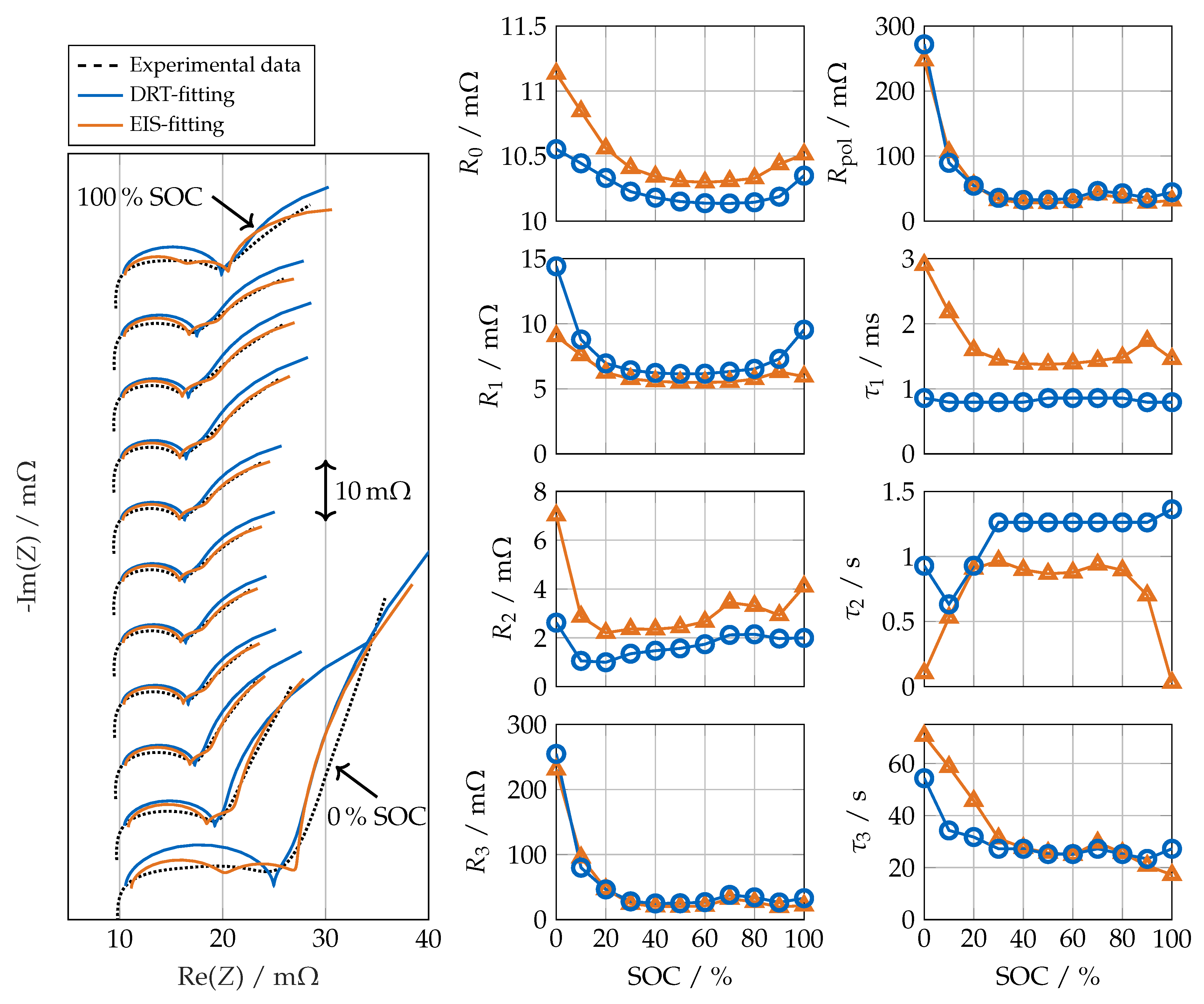
4.2. DRT-Fitting: Direct RC Parameterization from the DRT

We propose to estimate the RC parameters for an ECM directly from the DRT, making any additional fitting algorithms in the time or frequency-domain superfluous. This approach circumvents the manual specification of starting values and/or boundary conditions for these fitting algorithms and promotes physically meaningful parameter sets. Although our approach is not a fitting algorithm per se, and the RC parameters are determined analytically from the DRT, we call it DRT-fitting in analogy to conventional EIS-fitting (fitting RC parameters to impedance spectra) or pulse-fitting (fitting RC parameters to the time-domain current/voltage data). Since dynamic processes of the investigated system become visible as peaks in the DRT, the relaxation times ${\tau }_n$ of n RC elements can be chosen at the local maxima of $\gamma$. As stated in Equation (2), $\gamma$ is normalized to the total polarization resistance $R_{\mathrm{pol}}$. Therefore, the polarization resistance $R_n$ of a single relaxation process can be approximated by integrating between the adjacent minima of $\gamma$, labeled ${\tau }_a$ and ${\tau }_b$. Consequently, the parameters $R_n$ and $C_n$ of an RC element can be calculated as

$$\begin{array}{cc}\hfill R_n& ={\int }_{-{\tau }_a}^{{\tau }_b}\gamma (ln\tau )\mathrm{d}ln\tau ,\hfill \end{array}$$

(11)

$$\begin{array}{cc}\hfill C_n& =\frac{{\tau }_n}{R_n}.\hfill \end{array}$$

(12)

In engineering applications, the number of RC elements must often be defined a priori, notwithstanding the number of occurring processes in the DRT. This can corrupt the interpretability of RC parameters, when RC elements are not unambiguously correlated to the same electrochemical processes at all SOCs. On this account, Figure 4 proposes a flow chart of a decision logic for parameterizing RC elements directly from the DRT and takes into account the predefined number of RC elements. This process is henceforth denoted as DRT-fitting and is explained in the following.

Initially, all local maxima in the DRT are identified and labeled $P1$, while all inflection points are labeled $P2$. To identify the inflection points, the second derivative of $\gamma$ is consulted and ${\tau }_n$ is determined at the location of its maxima. The idea is that both geometric points indicate an underlying electrochemical process. We propose to associate one RC element to each primary process $P1$. If the predefined number of RC elements N matches the number of primary process $P1$, RC elements can be parameterized according to Equations (11) and (12) and the parameterization process has finished. If the DRT reveals more primary processes $P1$ than the predefined number of RC elements, the polarization resistance of the lowest peak is added to the process with the closest relaxation time. If the predefined number of RC elements exceeds the number of peaks in the DRT, the secondary processes $P2$ are associated to an additional RC element in descending order of the polarization resistance. In order to divide the polarization resistance between a secondary and a primary process, the integration limit is set to the point were the slope of $\gamma$ is lowest.

For our tested cell, the number of processes and their corresponding time constants was different at different SOCs. Hence, we ran the algorithm for the DRT of each tested SOC, in order to assure the consistent allocation of the same processes to the same RC elements over the entire SOC range.

4.3. Comparison to Conventional EIS-Fitting

To validate the proposed parameterization procedure (DRT-fitting), it is compared to a reference EIS-fitting algorithm. Conventional EIS-fitting was performed using a multistart algorithm [34] with 100 starting points to fit three RC elements to the measured impedance spectra in the frequency-domain. To ensure comparability of the results, we also only used EIS measurements to calculate the DRT and perform the DRT-fitting. Figure 5 shows the resulting parameters for R and $\tau$ and the corresponding impedance spectra compared to the measured ones.

The Nyquist plots indicate that both ECMs approximate the measured impedance spectra with similar accuracy. Between 10% SOC and 90% SOC both EIS-fitting and DRTfitting identify one process at the first semi-circle displaying the charge-transfer resistance, one process at the transition frequency and one process at the diffusion branch. While this is expected for the DRT-fitting, it is noticeable that the EIS-fitting algorithm allocates the three RC elements in the same manner. Besides minor offsets and shifts between individual RC elements, parameters of both methods coincide well with each other. At 0% SOC and 100% SOC the assignment of RC elements remains consistent for the DRT-fitting. This leads to the typical bathtub shape of the charge-transfer resistance [7]. The EIS-fitting algorithm, however, allocates the second RC elements to the second emerging charge-transfer process (P2). This leads to inconsistent RC parameters at the edges of the SOC area.

It needs to be noted that the boundaries of the EIS-fitting were set free, which could be changed in a way to force the algorithm to assign individual RC elements to certain frequency ranges. While both approaches lead to similar parameters in most cases, the advantage of the DRT-fitting is that it automatically determines physically reasonable and consistent parameters without a priori knowledge and the need for a manual, iterative, and time-consuming fixing of starting values and boundary conditions.

Since both approaches identify similar RC parameters, they also lead to a comparable accuracy in the validation cycle (Table 2), whereby the error of the DRT-fitting is slightly higher (in the range of few $\mathrm{m}\mathrm{V}$) for all validation regimes. It can be concluded that when using EIS data alone, the proposed DRT-fitting does not gain any improvements in accuracy compared to the conventional EIS-fitting algorithm. However, it allows for a convenient combination of EIS and TDM.

5. Combination of EIS and TDM

5.1. Merging Approaches

As reviewed in Section 1.2, there are already some approaches to combine both measurement domains. However, most of these use the the DRT only to gain a priori knowledge and subsequently perform conventional fitting.

In this work, we present and compare three different merging approaches, which occur at various stages during the parameterization process using either a subset of RC parameters (Separate DRT-fitting), intermediate results (Interconnected DRT-fitting) or raw measurement data (Combined DRT-fitting). All three employ the proposed DRT-fitting for direct RC parameterization from the DRT and without the need for any conventional fitting algorithm. The three approaches are illustrated in Figure 6, and are explained in the following:

1.

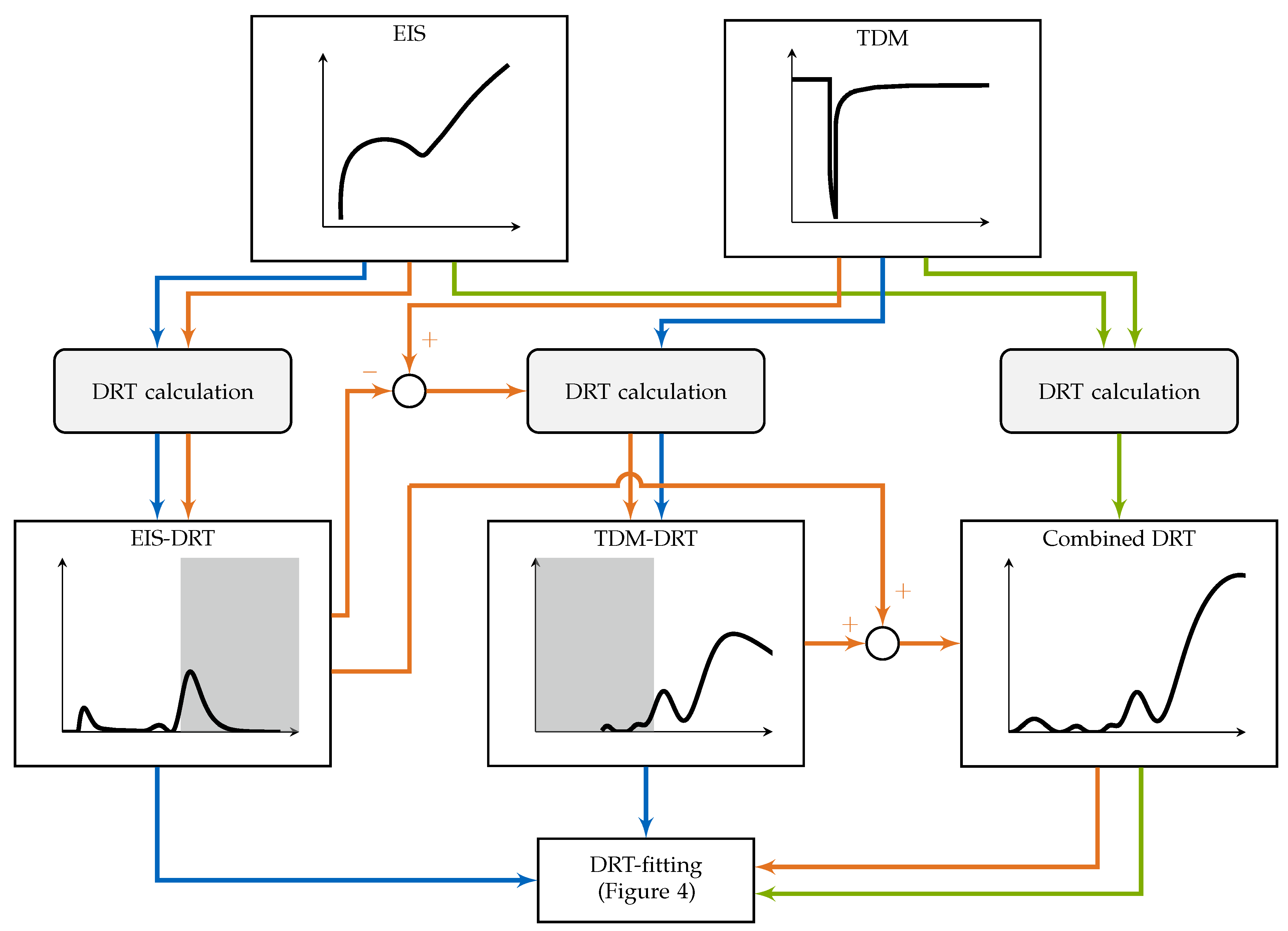
Separate DRT-fitting (blue):

In our first approach, EIS and TDM are used individually to parameterize different RC elements, the allocation of which is defined a priori. With this assumption, EIS and TDM are processed independent from each other. The ohmic resistance and the first RC elements (two in our case) are parameterized purely based on the EIS-DRT, whereas the remaining RC elements (two in our case) are determined from TDM-DRT only. Therefore, relaxation times higher than $\widehat{\tau }$, with $\widehat{\tau }$ being the highest relaxation time with a local minimum in the EIS-DRT, are ignored in the EIS-DRT. Likewise, the TDM-DRT is only evaluated at $\tau >\widehat{\tau }$. Depending on the sampling frequency, it is difficult to capture high-frequent loss processes during TDM, where meaningless oscillations can occur at low relaxation times close to $\widehat{\tau }$ of the TDM-DRT. This motivates an interconnected approach.

2.

Interconnected DRT-fitting (orange):

The goal of our second approach is to use information of EIS measurements in a more intertwined calculation of the TDM-DRT to avoid the described problems of meaningless oscillations at low relaxation times. Since the DRT equals a series of an infinite number of RC elements, the voltage relaxation which is caused by the high-frequency processes of the cell can be calculated from the EIS-DRT:

$$u_{\mathrm{EIS}}(t>(t_0+T_{\mathrm{p}}))={\int }_{-\infty }^{\infty }{\gamma }_{\mathrm{EIS}}(ln\tau )I_{\mathrm{p}}[exp\left(\frac{t_0+T_{\mathrm{p}}-t}{\tau }\right)-exp(-\frac{t_0-t}{\tau })]\mathrm{d}ln\tau .$$

(13)

This virtual voltage response is subtracted from the measured voltage of TDM. Since the EIS-DRT is only used to subtract the high-frequency behavior of the cell, the diffusive branch is removed from the impedance spectrum before evaluating Equation (13). Afterwards, the remaining voltage response is used to calculate the TDM-DRT according to Equation (7). Adding EIS-DRT and TDM-DRT finally yields a DRT of the complete system, which is used for the parameterization of all three RC elements. A disadvantage of this rather complex approach is that errors within calculation of the EIS-DRT propagate into the next step and will influence the voltage signal and thus also the TDM-DRT.

3.

Combined DRT-fitting (green):

Based on the disadvantages of the first two approaches, we developed a combined DRT-fitting, where the calculation of EIS-DRT and TDM-DRT is performed simultaneously in one single step. This makes decision of a border time constant $\widehat{\tau }$ superfluous and avoids complex interconnected fitting. Defining one system of equations in order to find $\gamma (ln\tau )$, such that it best fits both measurements, directly results in a DRT that displays the complete dynamic behavior of the measured cell from high to low frequencies. This can be implemented by merging Equations (3) and (7) to

$$\underset{U_{\mathrm{OCV}},R_0,\mathit{R}}{min}∥\sqrt{\mathit{w}}\left[\begin{array}{ccc}{\mathit{A}}_{\mathrm{Z}}^{\prime }& \mathbf{0}& \mathbf{1}\\ {\mathit{A}}_{\mathrm{Z}}^{″}& \mathbf{0}& \mathbf{0}\\ {\mathit{A}}_{\mathrm{u}}& \mathbf{1}& \mathbf{0}\end{array}\right]\left[\begin{array}{c}\mathit{R}\\ U_{\mathrm{OCV}}\\ R_0\end{array}\right]-{\sqrt{\mathit{w}}\left[\begin{array}{c}{\mathit{Z}}_{\exp }^{\prime }\\ {\mathit{Z}}_{\exp }^{″}\\ {\mathit{u}}_{\exp }\end{array}\right]∥}_2^2$$

(14)

$$\begin{array}{cccc}\hfill \underset{\mathit{x}}{min}\parallel {\mathit{B}}_{\mathrm{comb}}& \mathit{x}\hfill & \hfill -& {\mathit{D}}_{\exp }{\parallel }_2^2\hfill \end{array}$$

(15)

This equals a summation of the residuals of EIS-DRT and TDM-DRT. The diagonal Matrix $\mathit{w}$ applies a weighting between EIS and TDM data to achieve an equal influence of both measurements, the derivation of which can be found in Appendix D. Minimizing Equation (15) yields the DRT of the whole system as well as $R_0$ and $U_{OCV}$ and can thus be used to parameterize all ECM parameters at once.

The presented approaches are validated against a validation cycle in the time-domain in the following.

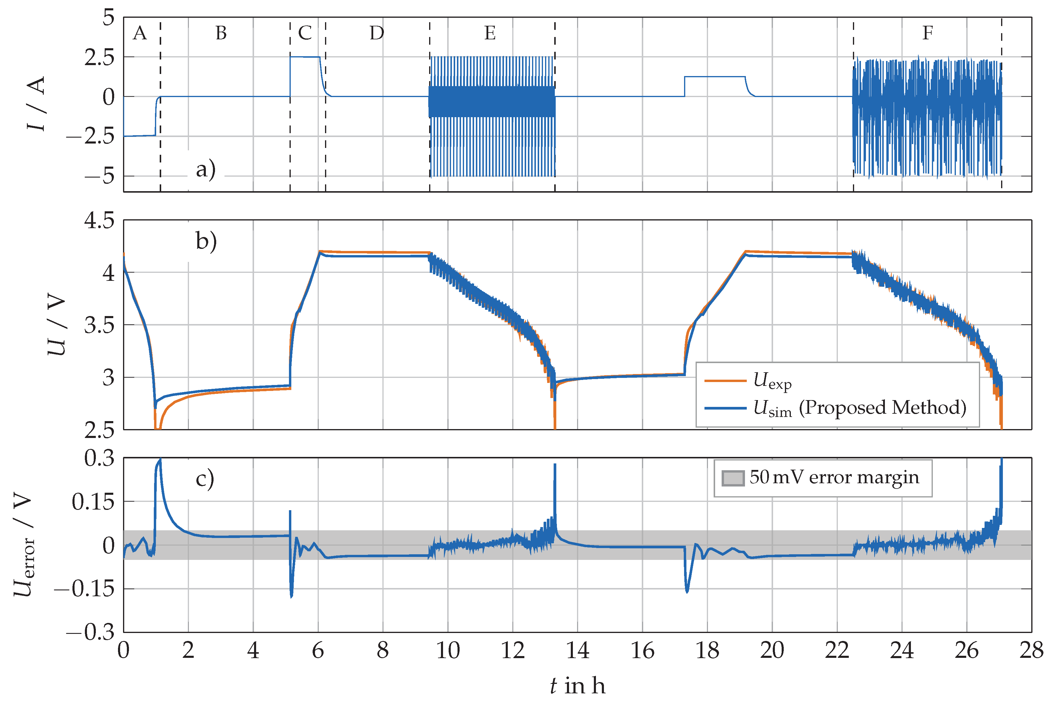
5.2. Validation Results

We validated our method by comparing the measured voltage with the simulated voltage during a validation cycle with a defined current profile (Figure 7a). The validation cycle started with a CCCV discharge (A) and charge (C) at 1 C with 4 $\mathrm{h}$ relaxation (B) after the discharge and 3 $\mathrm{h}$ relaxation (D) after the charge phase. This was followed by a DST (E), in which the cell was discharged by a sequence of short charge and discharge pulses between $-2$ C and 1 C. Finally, after charging the cell back to 100% SOC, a real driving cycle, recorded with a Volkswagen eGolf (F), was repeated until the lower cut-off voltage was reached.

In

Table 2. Comparison of the RMSE in $\mathrm{mV}$ during the validation cycle of different RC parameter sets.

	EIS-Fitting	DRT-Fitting	DRT-Fitting
Measurement	EIS	EIS	EIS and TDM
Merging Approach	n.a.	n.a.	Separate	Interconnected	Combined
Regularization Term	n.a.	x	x/$\frac{{\mathit{d}}^2\mathit{x}}{\mathit{d}ln(\mathit{\tau }{)}^2}$	x/$\frac{{\mathit{d}}^2\mathit{x}}{\mathit{d}ln(\mathit{\tau }{)}^2}$	$\frac{{\mathit{d}}^2\mathit{x}}{\mathit{d}ln(\mathit{\tau }{)}^2}$
Whole Validation Cycle	72.56	73.14	45.18	41.52	43.38
A: 1 C Discharge	42.88	46.76	28.78	26.41	26.71
B: Relaxation at 0% SOC	148.12	148.17	38.86	52.44	56.87
C: 1 C Charge	49.61	56.85	95.08	60.87	59.63
D: Relaxation at 100% SOC	37.35	37.35	36.33	36.47	36.74
E: DST	24.14	25.63	22.65	20.59	22.16
F: Driving Profile	31.56	32.05	23.69	25.12	27.39

, the root mean square error (RMSE) of the different configurations of the proposed DRT-fitting as well as the conventional EIS-fitting is listed for the whole validation cycle and for the different segments A–F separately. Exemplary, Figure 7b) shows the measured and simulated voltage of the combined DRT-fitting, where the DRT is calculated from EIS and TDM simultaneously during the validation cycle. In Figure 7c), the corresponding residual voltage $U_{\mathrm{error}}$ = $U_{\mathrm{sim}}$−$U_{\exp }$ is plotted.

It can be seen that adding TDMs to the parameterization process by using our proposed merging approaches significantly improved the results compared to the conventional EIS-fitting. The lowest overall RMSE ($41.52$ $\mathrm{m}$$\mathrm{V}$) was reached by the interconnected DRT-fitting with a relative improvement of 42% compared to the conventional EIS-fitting. Thereby, the differences of the three merging approaches were comparably low (in the range of a few mVs for most regimes). The only big difference occurred at 0% SOC and at the beginning of the charging phase, when using the separate DRT-fitting. In this configuration, apparently, different loss processes were assigned to the RC elements in this region. The RMSE was lower compared to the interconnected and combined DRT-fitting during the relaxation phase and higher at the beginning of the charging phase. The magnitude of the voltage error at 0% SOC and 100% SOC was influenced by the OCV-SOC relationship in this region anyway, as revealed by the strong hysteresis until approx. 20% SOC (Section 2.3).

The voltage error in Figure 7c lay within the 50 $\mathrm{m}\mathrm{V}$ error margin for most of the time. Only at low SOC, at the end of discharging and at the beginning of charging, the error increased strongly. As discussed before, the high error in the low SOC range could mainly be attributed to the strong hysteresis, which was not modeled in our ECM. Therefore, in the future, more detailed investigations on the modeling of hysteresis are needed to further improve the simulation results, especially for modern LIB with silicon added to anode active material. It needs to be noted that we completely discharged the cell with a CCCV profile applying a low cut-off current of C/50. For most applications, however, such as battery electric vehicles, this low SOC area is of minor importance, since the SOC range is limited for various reasons such as safety or degradation [35].

6. Conclusions

In this study, we presented and validated a novel parameterization process for RC elements of ECMs. The main advantages of this approach can be summarized as follows: (1) merging of frequency- and time-domain measurement data to cover a broad frequency range, (2) automated DRT calculation using Tikhonov regularization and the L-curve criterion, and (3) RC parameterization directly from the DRT (DRT-fitting). Furthermore, we can conclude the following from our investigations.

To cover a broad frequency range of the cell’s dynamic behavior we utilize both measurements in the frequency-domain (EIS) and measurements in the time-domain (pulse-relaxation measurements). The TDMs, which in general are necessary to capture the low-frequency loss processes of the LIB, have shown that a long relaxation period of more than two weeks was necessary prior to the pulse-relaxation measurement itself. This was to eliminate all effects of bringing the cell to its respective SOC. Only when a fully relaxed state has been reached prior to the pulse-relaxation measurement does the procedure solely capture the cell’s kinetics and is not biased by any former excitation of the cell.

We investigated different regularization terms in the Tikhonov regularization to stabilize the DRT problem. Besides standard regularization with the solution norm itself, regularization with the norm of the solution’s first and second derivative were applied in the calculation of the DRT. The results have shown that in contrast to the EIS-DRT, where the standard regularization showed the best results, using the solution’s second derivative leads to an improved deconvolution of the TDM-DRT. During all DRT calculations, the Lcurve criterion has successfully been used to find the optimum regularization factor.

We showed that it is possible to determine RC parameters directly from the DRT without the use of any conventional optimization algorithm. The parameters resulting from the DRT-fitting are, with minor differences, comparable to a benchmark EIS-fitting. However, our approach avoids time-consuming work of setting boundary conditions and initial guesses for the fitting algorithm to achieve reasonable and consistent parameters over broad operating conditions.

Additionally, direct DRT-fitting allows for convenient merging of frequency and timedomain data. Therefore, we ultimately compared three methods of combining EIS and TDM data to be used in the proposed DRT-fitting. During a comprehensive validation cycle, all three methods achieved comparable results in most regions. However, they show a strong improvement compared to the conventional EIS-fitting—the RMSE was reduced by over 40%. Modeling of the cell at a low SOC proved to be most difficult for all methods, therefore detailed investigations of the hysteresis behavior are suggested for future work.

Furthermore, it should be kept in mind that the DRT calculation and the ECM parameterization in general is subject to several other influencing factors, which were not further investigated in this work. These include, for example, the range and number of relaxation times in the DRT, the definition of the minimization problem itself (like including an inductance or fixing the $U_{\mathrm{OCV}}$ or the $R_0$ value in the cost function), or applying a different measurement routine. For the TDMs especially, the impact of different measurement protocols should be further investigated. In the introduced ECM parameterization process, the allocation of the total polarization process to the RC elements as well as the number of RC elements have an important influence. Last but not least, validation of models is always dependent on the validation cycle, as shown by the separate evaluation of the different cycle regimes. In this work, we performed parameterization and validation only at 20 °C. In the future, this must be extended to account for the mutual dependency between dynamic loss process and heat generation inside the cell.

References

- Wassiliadis, N.; Adermann, J.; Frericks, A.; Pak, M.; Reiter, C.; Lohmann, B.; Lienkamp, M. Revisiting the dual extended Kalman filter for battery state-of-charge and state-of-health estimation: A use-case life cycle analysis. J. Energy Storage 2018, 19, 73–87. [Google Scholar] [CrossRef]
- Birkl, C.R.; Roberts, M.R.; McTurk, E.; Bruce, P.G.; Howey, D.A. Degradation diagnostics for lithium ion cells. J. Power Sources 2017, 341, 373–386. [Google Scholar] [CrossRef]
- Schmitt, J.; Maheshwari, A.; Heck, M.; Lux, S.; Vetter, M. Impedance change and capacity fade of lithium nickel manganese cobalt oxide-based batteries during calendar aging. J. Power Sources 2017, 353, 183–194. [Google Scholar] [CrossRef]
- Zhou, X.; Huang, J.; Pan, Z.; Ouyang, M. Impedance characterization of lithium-ion batteries aging under high-temperature cycling: Importance of electrolyte-phase diffusion. J. Power Sources 2019, 426, 216–222. [Google Scholar] [CrossRef]
- Bruch, M.; Millet, L.; Kowal, J.; Vetter, M. Novel method for the parameterization of a reliable equivalent circuit model for the precise simulation of a battery cell’s electric behavior. J. Power Sources 2021, 490. [Google Scholar] [CrossRef]
- Karger, A.; Wildfeuer, L.; Maheshwari, A.; Wassiliadis, N.; Lienkamp, M. Novel method for the on-line estimation of low-frequency impedance of lithium-ion batteries. J. Energy Storage 2020, 32, 101818. [Google Scholar] [CrossRef]
- Gantenbein, S.; Weiss, M.; Ivers-Tiffée, E. Impedance based time-domain modeling of lithium-ion batteries: Part I. J. Power Sources 2018, 379, 317–327. [Google Scholar] [CrossRef]
- Ciucci, F. Modeling electrochemical impedance spectroscopy. Curr. Opin. Electrochem. 2019, 13, 132–139. [Google Scholar] [CrossRef]
- Waag, W.; Fleischer, C.; Sauer, D.U. On-line estimation of lithium-ion battery impedance parameters using a novel varied-parameters approach. J. Power Sources 2013, 237, 260–269. [Google Scholar] [CrossRef]
- Schmidt, R. Impedance Spectroscopy of Electroceramics. In Ceramic Materials Research Trends; Lin, P.B., Aguiar, R., Eds.; Nova Science Publ.: New York, NY, USA, 2007. [Google Scholar]
- Schönleber, M.; Klotz, D.; Ivers-Tiffée, E. A Method for Improving the Robustness of linear Kramers-Kronig Validity Tests. Electrochim. Acta 2014, 131, 20–27. [Google Scholar] [CrossRef]
- Witzenhausen, H. Elektrische Batteriespeichermodelle: Modellbildung, Parameteridentifikation und Modellreduktion. Ph.D. Thesis, Rheinisch-Westfälischen Technischen Hochschule Aachen, Aachen, Germany, 2017. [Google Scholar]
- Illig, J.; Ender, M.; Chrobak, T.; Schmidt, J.P.; Klotz, D.; Ivers-Tiffée, E. Separation of Charge Transfer and Contact Resistance in LiFePO4-Cathodes by Impedance Modeling. J. Electrochem. Soc. 2012, 159, A952–A960. [Google Scholar] [CrossRef]
- Schmidt, J.P.; Berg, P.; Schönleber, M.; Weber, A.; Ivers-Tiffée, E. The distribution of relaxation times as basis for generalized time-domain models for Li-ion batteries. J. Power Sources 2013, 221, 70–77. [Google Scholar] [CrossRef]
- Sabet, P.S.; Stahl, G.; Sauer, D.U. Non-invasive investigation of predominant processes in the impedance spectra of high energy lithium-ion batteries with Nickel-Cobalt-Aluminum cathodes. J. Power Sources 2018, 406, 185–193. [Google Scholar] [CrossRef]
- Schichlein, H.; Müller, A.C.; Voigts, M.; Krügel, A.; Ivers-Tiffée, E. Deconvolution of electrochemical impedance spectra for the identification of electrode reaction mechanisms in solid oxide fuel cells. J. Appl. Electrochem. 2002, 32, 875–882. [Google Scholar] [CrossRef]
- Hershkovitz, S.; Baltianski, S.; Tsur, Y. Harnessing evolutionary programming for impedance spectroscopy analysis: A case study of mixed ionic-electronic conductors. Solid State Ionics 2011, 188, 104–109. [Google Scholar] [CrossRef]
- Goldammer, E.; Kowal, J. Determination of the Distribution of Relaxation Times by Means of Pulse Evaluation for Offline and Online Diagnosis of Lithium-Ion Batteries. Batteries 2021, 7, 36. [Google Scholar] [CrossRef]
- Lain, M.J.; Brandon, J.; Kendrick, E. Design strategies for high power vs. High energy lithium ion cells. Batteries 2019, 5, 64. [Google Scholar] [CrossRef] [Green Version]
- Schmidt, J.P. Verfahren zur Charakterisierung und Modellierung von Lithium-Ionen Zellen; Karlsruher Institut für Technologie: Karlsruhe, Germany, 2013. [Google Scholar]
- Schmidt, J.P.; Ivers-Tiffée, E. Pulse-fitting—A novel method for the evaluation of pulse measurements, demonstrated for the low frequency behavior of lithium-ion cells. J. Power Sources 2016, 315, 316–323. [Google Scholar] [CrossRef]
- Sturm, J.; Rheinfeld, A.; Zilberman, I.; Spingler, F.; Kosch, S.; Frie, F.; Jossen, A. Modeling and simulation of inhomogeneities in a 18650 nickel-rich, silicon-graphite lithium-ion cell during fast charging. J. Power Sources 2019, 412, 204–223. [Google Scholar] [CrossRef] [Green Version]
- Klotz, D. Characterization and Modeling of Electrochemical Energy Conversion Systems by Impedance Techniques; KIT Scientific Publishing: Karlsruhe, Germany, 2012. [Google Scholar]
- Schichlein, H. Experimentelle Modellbildung für die Hochtemperatur-Brennstoffzelle SOFC; Universität Karlsruhe (TH): Aachen, Germany, 2003. [Google Scholar]
- Wan, T.H.; Saccoccio, M.; Chen, C.; Ciucci, F. Influence of the Discretization Methods on the Distribution of Relaxation Times Deconvolution: Implementing Radial Basis Functions with DRTtools. Electrochim. Acta 2015, 184, 483–499. [Google Scholar] [CrossRef]
- Boukamp, B.A. A Linear Kronig-Kramers Transform Test for Immittance Data Validation. J. Electrochem. Soc. 1995, 142, 1885. [Google Scholar] [CrossRef]
- Saccoccio, M.; Wan, T.H.; Chen, C.; Ciucci, F. Optimal Regularization in Distribution of Relaxation Times applied to Electrochemical Impedance Spectroscopy: Ridge and Lasso Regression Methods—A Theoretical and Experimental Study. Electrochim. Acta 2014, 147, 470–482. [Google Scholar] [CrossRef]
- Tikhonov, A.N.; Goncharsky, A.V.; Hazewinkel, M. Numerical Methods for the Solution of Ill-Posed Problems; Springer: Dordrecht, The Netherlands, 2010. [Google Scholar]
- Hahn, M.; Schindler, S.; Triebs, L.C.; Danzer, M.A. Optimized Process Parameters for a Reproducible Distribution of Relaxation Times Analysis of Electrochemical Systems. Batteries 2019, 5, 43. [Google Scholar] [CrossRef] [Green Version]
- Hansen, P.C. Analysis of Discrete Ill-Posed Problems by Means of the L-Curve. SIAM Rev. 1992, 34, 561–580. [Google Scholar] [CrossRef]
- Hansen, P.C. The L-Curve and Its Use in the Numerical Treatment of Inverse Problems. Available online: https://orbit.dtu.dk/en/publications/the-l-curve-and-its-use-in-the-numerical-treatment-of-inverse-pro-2 (accessed on 18 May 2021).
- Choi, M.B.; Shin, J.; Ji, H.I.; Kim, H.; Son, J.W.; Lee, J.H.; Kim, B.K.; Lee, H.W.; Yoon, K.J. Interpretation of Impedance Spectra of Solid Oxide Fuel Cells: L-Curve Criterion for Determination of Regularization Parameter in Distribution Function of Relaxation Times Technique. JOM 2019, 71, 3825–3834. [Google Scholar] [CrossRef]
- Press, W.H. Numerical Recipes in C: The Art of Scientific Computing, 2nd ed.; Reprinted with Corr. to Software Version 2.10; Cambridge University Press: Cambridge, UK, 2002. [Google Scholar]
- The MathWorks Inc. MATLAB MultiStart. 2021. Available online: https://de.mathworks.com/help/gads/multistart.html (accessed on 5 May 2021).
- Reiter, C.; Wassiliadis, N.; Wildfeuer, L.; Wurster, T.; Lienkamp, M. Range Extension of Electric Vehicles through Improved Battery Capacity Utilization: Potentials, Risks and Strategies. In Proceedings of the 2018 21st International Conference on Intelligent Transportation Systems (ITSC), Maui, HI, USA, 4–7 November 2018; pp. 321–326. [Google Scholar] [CrossRef]
- Sonn, V.; Leonide, A.; Ivers-Tiffée, E. Combined deconvolution and CNLS fitting approach applied on the impedance response of technical Ni/ 8YSZ cermet electrodes. J. Electrochem. Soc. 2008, 155, B675–B679. [Google Scholar] [CrossRef]
- Franklin, A.D.; de Bruin, H.J. The fourier analysis of impedance spectra for electroded solid electrolytes. Phys. Status Solidi (a) 1983, 75, 647–656. [Google Scholar] [CrossRef]
- Hust, F.; Witzenhausen, H.; Sauer, D.U. Distribution of relaxation times for lithium-ion batteries. In Proceedings of the 9th International Symposium on Electrochemical Impedance Spectroscopy, Okinawa, Japan, 17–20 June 2013. [Google Scholar]
- Tesler, A.B.; Lewin, D.R.; Baltianski, S.; Tsur, Y. Analyzing results of impedance spectroscopy using novel evolutionary programming techniques. J. Electroceram. 2010, 24, 245–260. [Google Scholar] [CrossRef]
- Tuncer, E.; Macdonald, J.R. Comparison of methods for estimating continuous distributions of relaxation times. J. Appl. Phys. 2006, 99, 074106. [Google Scholar] [CrossRef] [Green Version]