
Detection of Brominated Plastics from E-Waste by Short-Wave Infrared Spectroscopy
by
 , ,
, ,
Giuseppe Bonifazi
1,2 ,
,
Ludovica Fiore
1,
Riccardo Gasbarrone
1,
Pierre Hennebert
3 and
Silvia Serranti
1,2,* 1
Department of Chemical Engineering, Materials & Environment, Sapienza University of Rome, Via Eudossiana 18, 00184 Rome, Italy
2
Research Center for Biophotonics, Sapienza University of Rome, Polo Pontino, Corso della Repubblica 79, 04100 Latina, Italy
3
INERIS, French National Institute for Industrial Environment and Risks CS 10440, CEDEX 03, 13592 Aix-en-Provence, France
*
Author to whom correspondence should be addressed.
Recycling 2021, 6(3), 54; https://0-doi-org.brum.beds.ac.uk/10.3390/recycling6030054
Submission received: 31 July 2021
/
Revised: 20 August 2021
/
Accepted: 23 August 2021
/
Published: 25 August 2021
(This article belongs to the Special Issue Exclusive Papers of the Editorial Board Members (EBMs) of Recycling)
Abstract
:In this work, the application of Short-Wave Infrared (SWIR: 1000–2500 nm) spectroscopy was evaluated to identify plastic waste containing brominated flame retardants (BFRs) using two different technologies: a portable spectroradiometer, providing spectra of single spots, and a hyperspectral imaging (HSI) platform, acquiring spectral images. X-ray Fluorescence (XRF) analysis was preliminarily performed on plastic scraps to analyze their bromine content. Chemometric methods were then applied to identify brominated plastics and polymer types. Principal Component Analysis (PCA) was carried out to explore collected data and define the best preprocessing strategies, followed by Partial Least Squares—Discriminant Analysis (PLS-DA), used as a classification method. Plastic fragments were classified into “High Br content” (Br > 2000 mg/kg) and “Low Br content” (Br < 2000 mg/kg). The identified polymers were acrylonitrile butadiene styrene (ABS) and polystyrene (PS). Correct recognition of 89–90%, independently from the applied technique, was achieved for brominated plastics, whereas a correct recognition ranging from 81 to 89% for polymer type was reached. The study demonstrated as a systematic utilization of both the approaches at the industrial level and/or at laboratory scale for quality control can be envisaged especially considering their ease of use and the short detection response.
1. Introduction
In recent years, the management of Waste from Electrical and Electronic Equipment (WEEE) is becoming more and more challenging due to its growing volume rate [1]. WEEE waste streams require special treatment and sometimes complex management activities due to their intrinsic potential toxicity for the environment and their harmfulness to human and animal health [2]. Their complexity in terms of composition, which may vary in time according to technological improvement and environmental regulations, lead to difficulties in recycling and recovery processes.
WEEE contain important metals (i.e., gold, silver, iron, steel, copper, and aluminum) and other valuable materials, such as plastics, glass, and wood [3]. Their correct handling, in terms of processing actions to obtain raw materials of secondary origins [4], thus produces a positive impact both in an economic (i.e., materials recovery) and in an environmental (i.e., reduced material disposed-off or incinerated) perspective.
In Europe, the plastic recycling rate ranges between 26 and 52% [5], showing that there is a need to increase such rates, developing innovative strategies. Considering that plastics from WEEE represent on average 25% of all WEEE annually generated by weight [6], their correct recycling can represent a valuable resource of secondary polymers if properly processed. One of the main difficulties in WEEE plastic recovery is the presence of different types of plastics and additives as well as flame retardants, colorants, stabilizers, and other chemicals [7].
More than 15 types of plastics can be found in WEEE [8]. The most abundant polymers are acrylonitrile–butadiene–styrene (ABS), polystyrene (PS), high-impact polystyrene (HIPS), blends of polycarbonate (PC/ABS), and polypropylene (PP) [6]. In more detail, styrene-based polymers represent about 50% of all WEEE plastics [9].
In Electrical and Electronic Equipment (EEE), polymers can be compounded with organic or inorganic materials, particulates, or fiber fillers [10], or mixed together to improve the properties of the final product. Plastics, when utilized in EEE, are added with flame retardants (FRs) in order to meet product flammability performance standards [11]. It is estimated that about 40% of all FRs found in WEEE are brominated flame retardants (BFRs) [12], and about 9% of WEEE plastics contain BFRs [6].
A study developed in 2017 reported as about 39% of Small Household Appliances (SHA), Cathode Ray Tubes (CRT), and flat screens were realized utilizing brominated polymers. About 26% of SHA presented at least one plastic element added with BFRs, and only 15% did not present any brominated polymers. In 2015, the bromine (Br) presence of regulated brominated substances was identified to be up to 86% of total bromine in “older” waste (i.e., SHA and CRT), about 30–50% in “younger” waste (i.e., flat screens) and only 8% in recent products (2009–2013) [13].
There are about 75 different commercial BFRs [14]. The most used in EEE are tetrabromobisphenol–A (TBBPA) and polybrominated diphenyl ethers (PBDE) [15]. BFRs are lipophilic, persistent, and bio-accumulative compounds that can cause serious damage to human health (such as endocrine destruction, damage to the thyroid, growth/development, and reproduction) and the environment [16]. For these reasons, the use of some BFRs has been banned or restricted by European Union [17,18]. It is evident the arising importance, in a recycling process, of separating polymers containing BFRs from those without BFRs [10]. The presence of BFRs in WEEE polymers can compromise the entire recycling process, negatively affecting the quality of the recycled plastic stream, whose re-utilization, as previously mentioned, can cause serious health problems. Some studies [19,20,21] have revealed, in fact, the presence of BFRs in food packaging, this contamination being associated with recycled plastic materials potentially derived from WEEE.
In order to improve the quality of the products obtained from plastic waste, it is thus necessary to remove the fraction containing added BFRs. In a sorting scenario, a technical specification [22] recommends the separation of WEEE plastics with a Br concentration > 2000 mg/kg from the other plastics (BFRs free plastics). A correct WEEE plastic sorting can thus dramatically increase the quality and the overall commercial value of recovered materials.
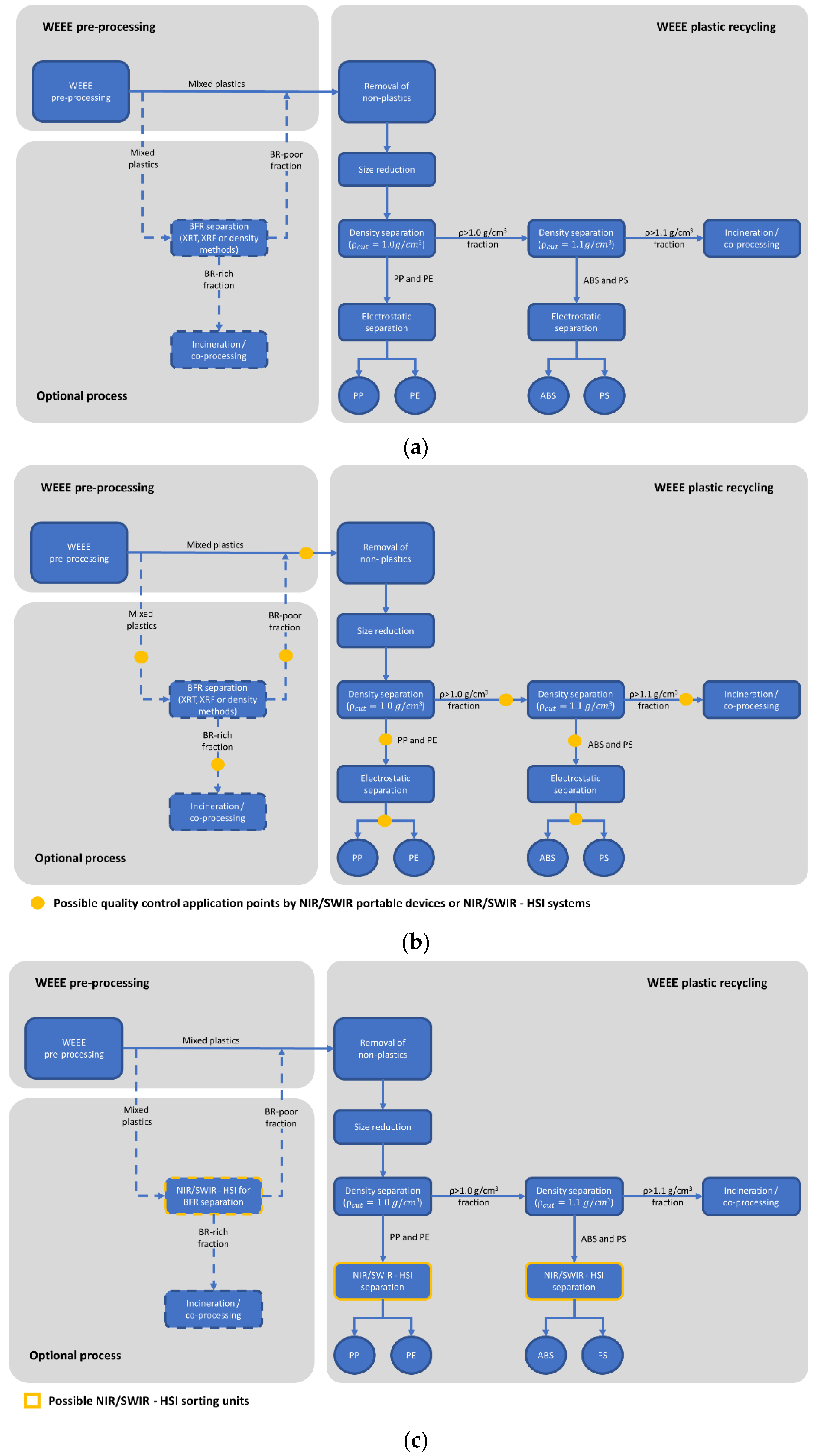
WEEE plastic fractions are first cleaned of their nonpolymeric impurities (e.g., wood, paper, minerals, metals), then they are shredded and, finally, subjected to a density separation (i.e., sink and float process). The conventional WEEE plastic treatment process layouts are shown in Figure 1a [6].
The density method is thus one of the main used separation techniques to sort brominated from not brominated plastics [13]. Usually, the separation of these plastics is carried out by a dense medium, typically assuming as cut density the value of 1.1 g/cm3. Most of the Br-containing particles are usually concentrated into the ‘heavies’ (sink) fraction (ρ > 1.1 g/cm3). Typically, two density sorting steps are applied in order to create three fractions, [6], that is: (i) one fraction with a density lower than 1 g/cm3, containing additive-poor polyolefins (PP and PE), (ii) one fraction with a density 1.0–1.1 g/cm3 containing additive-poor ABS and PS and (iii) one with a density higher than 1.1 g/cm3 containing polymers with BFRs.
The first two fractions can be then further sorted using electrostatic separation methods, whereas the last fraction, with a density higher than 1.1 g/cm3, is typically disposed of by incineration, co-processing in cement kilns, or landfilled, and generally classified as hazardous waste.
However, the density method, despite its routine use in separating brominated plastics, is affected by errors, including plastics with high Br content in the recycled low Br plastic stream (floating fraction) and losing profitably recoverable plastics in the sink fraction, due to the presence of polymers with similar densities, such as ABS and PS [6,23]. Indeed, the sink-float method suffers from relatively poor selectivity. In more detail, plastics sorting from CRT screens using this method produces a waste fraction (Br-rich fraction) representing about 30% of the input [6].
The fast identification of polymers with certain flame-retardant grades in a mixed waste stream is not an easy task. The methods used at laboratory scale to detect flame retardant grades of polymers are commonly based on the utilization of different spectroscopic techniques [24], the most utilized include Raman scattering, mass pyrolysis, sliding spark (spark ablation), X-ray Fluorescence (XRF), Laser-Induced Plasma Spectroscopy (LIPS), Near Infrared (NIR), Short-Wave Infrared (SWIR), Mid Infrared (MIR) reflection, MIR pyrolysis and MIR Acousto–Optic Tunable Filter (MIR AOTF).
However, not all the above-mentioned methods are fast, sustainable, not destructive, and cost-effective. In a plant scenario, a method that is rapid, effective, and does not require sample preparation is needed. NIR-SWIR spectroscopy meets these requirements.
In recent years, Hyperspectral Imaging (HSI) has rapidly emerged and fast grown in many industrial fields, including the solid waste sector [25,26]. HSI is a technology allowing the collection of both spatial and spectral information at the same time, thus providing several physical and chemical characteristics of the analyzed material [27]. In literature, several studies related to NIR–his-based applications for WEEE material detection [28,29,30,31,32] and polymer identification and/or characterization [33,34,35,36,37,38,39,40] are reported.
In this work, two different spectroscopic techniques, working in the SWIR range (1000–2500 nm), were applied to identify brominated plastic scraps from CRT monitors and televisions, adopting a multi-analytical approach: a portable spectrophotoradiometer, working on “single spot base” and a HSI platform, acquiring spectral images. The first one was evaluated in order to perform a rapid test on batch samples collected in the feed and/or on some of the plastic waste flow streams generated by the recycling process, as schematically represented in Figure 1b. The second one was tested for the “on-line” assessment of sorted plastic quality, with reference to the BFRs presence, and for the development of sorting strategies, as the example reported in Figure 1c.
2. Materials and Methods
2.1. Materials
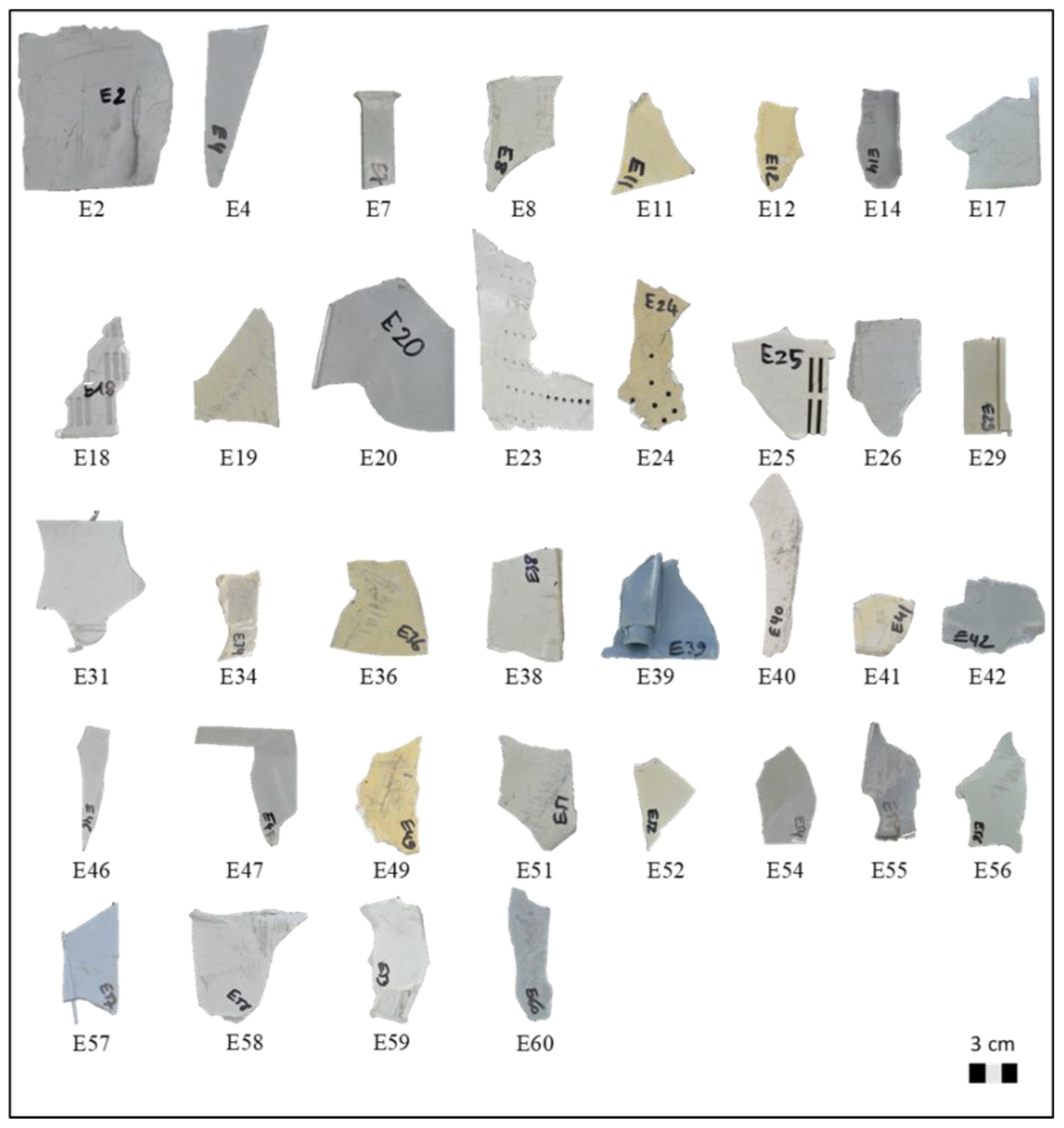
The analyzed plastic samples were collected from the recycling plant of Galloo Plastics (Halluin, France), in which density medium separation is used for concentrating the BFRs plastics from a WEEE stream. The samples consisted of shredded plastic scraps from cathode ray tube (CRT) monitors and televisions. The physical features (i.e., color, thickness, and weight) of the samples are reported in Table 1. In more detail, scraps were mainly made of acrylonitrile butadiene styrene (ABS) and polystyrene (PS) polymers with variable bromine content. Thirty-six scraps (Figure 2) were randomly selected from the samples, and their polymer typology (ABS and PS) was verified using Raman spectroscopy.
2.2. Methods
2.2.1. X-ray Fluorescence Analysis
The scraps were preliminary analyzed to determine the total bromine content by a portable XRF spectrometer. This procedure was adopted, as it is commonly used in recycling plants, to perform controls on plastic scraps which could contain BFRs added polymers.
A hand-held XRF Niton™ XL2 (Thermo Fisher Scientific Inc. Waltham, MA, USA), with a silver anode X-ray Tube (6–45 kV, 1–200 uA, 2 W max) mounted on a benchtop stand aided by software dedicated for plastics (with automatic thickness correction) was used for Br measurements. Measurement time for each individual scrap was about 60 s. Preliminary tests have been carried out in order to verify the robustness of XRF determinations. To reach this goal, Br determinations were performed on a certified reference material during different days at a Br concentration of about 1000 mg/kg. A value of 0.03 was thus obtained for the Coefficient of Variation (CV), where CV is the ratio of Standard Deviation (SD) to the Mean (M) collected data.
According to the detected Br contents, individual scraps were then divided into two representative sample sets: one for training and another for validation.
2.2.2. SWIR Spectral Analysis
Portable spectroradiometer. Spectra acquisitions were performed in reflectance mode for each individual scrap, using the ASD FieldSpec® 4 Standard-Res field portable spectroradiometer (ASD Inc., Boulder, CO, USA) with a contact probe. This portable instrument, working in VIS–SWIR regions (350–2500 nm), had a spectral resolution of 3 nm at 700 nm and 10 nm at 1400/2100 nm [41]. The spectroradiometer was composed of a detector unit and a fiber optics cable connected to a contact probe, controlled by a personal computer. The detector unit was realized by coupling different separate holographic diffraction gratings with three separate detectors. The detector architecture consisted of a VNIR detector (512 element silicon array: 350–1000 nm), a SWIR1 detector (Graded Index InGaAs. Photodiode, Two Stage TE Cooled; 1001–1800 nm), and a SWIR2 detector (Graded Index InGaAs. Photodiode, Two Stage TE Cooled; 1801–2500 nm). The ASD Contact Probe consisted of a halogen bulb light source with a color temperature 2901 +/− 10% °K. The contact probe spot size was 10 mm in diameter. Data acquisition and calibration procedures were performed using the ASD RS3 software (ASD Inc., Boulder, CO, USA) [42]. The calibration of the ASD FieldSpec® 4 Standard-Res spectroradiometer was performed by dark acquisition, calculated referencing the dark current calibration file, and by mean of the white reference measurement, acquiring a standardized white Spectralon® ceramic material. After this calibration stage, the spectrum was acquired, and reflectance was then computed for each sample. For the purposes of this study, only the SWIR range of the collected spectra was investigated.
Hyperspectral imaging. Hyperspectral images were acquired in the SWIR range (1000–2500 nm) using the SisuCHEMATM XL Chemical Imaging Workstation (Specim, Spectral Imaging Ltd., Oulu, Finland), equipped with the ImSpectorTM N25E imaging spectrograph (Specim, Spectral Imaging Ltd., Oulu, Finland). A 31 mm lens with a field of view of 50 mm was adopted. The spectral resolution was 10 nm. This device combined NIR spectroscopy with high-resolution imaging. A push-broom hyperspectral camera acquired and built the hyperspectral image of sample line by line, simultaneously acquiring all wavelengths for each line. Image data were automatically calibrated in reflectance by measuring an internal standard reference target before each sample scan. A comparison between the technical characteristics of the two spectral devices is reported in Table 2.
2.2.3. Experimental Procedure
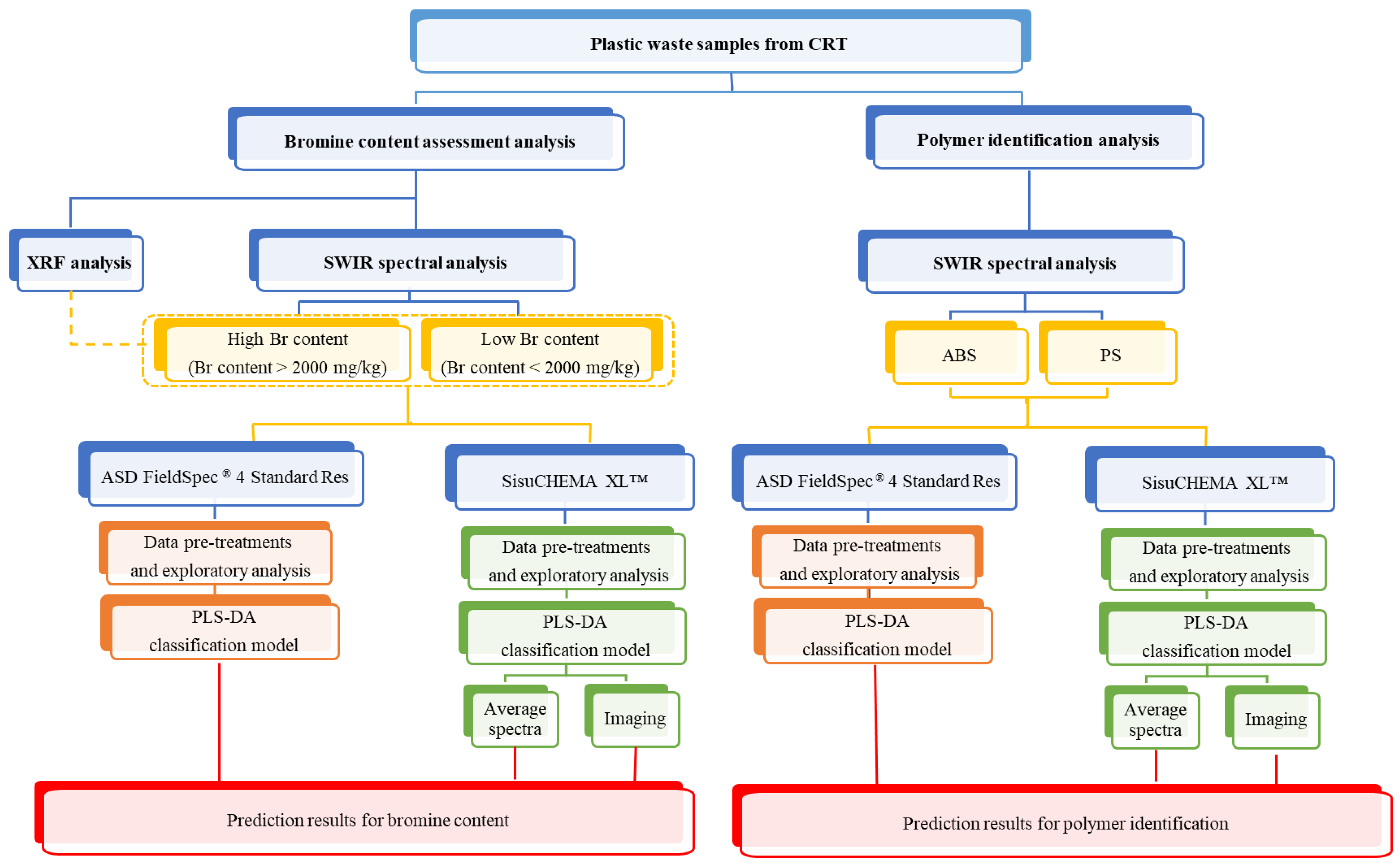
The flow chart reported in Figure 3 schematically explains the experimental procedure defined to perform the analysis using the different sensing devices and detection architectures. Two sample sets, belonging to different polymer families (ABS and PS) and characterized by different bromine content, “High Br content” (Br > 2000 mg/kg) and “Low Br content” (Br < 2000 mg/kg), were thus investigated.
Data acquisition and handling. The data collected by XRF analysis were used to set reference classes for SWIR investigation.
ASD FieldSpec® 4 Standard-Res spectra “.asd” data files were stacked into an ASCII text file using ViewSpec Pro (ver. 6.2.0; ASD Inc., Boulder, CO, USA). The ASCII text file was then imported into the MATLAB® environment (MATLAB R2019a ver. 9.6.0; The Mathworks, Inc., Natick, MA, USA) using “fieldspec_import3.m”, an ad hoc written script [43]. Imported data files were analyzed using Eigenvector Research, Inc. PLS_toolbox (ver. 8.6; Eigenvector Research, Inc, Wenatchee, WA, USA) within the MATLAB® environment. Hyperspectral images were also imported into the MATLAB® environment and subsequently analyzed with the aid of PLS_toolbox and MIA_toolbox (ver. 3.0; Eigenvector Research, Inc, Wenatchee, WA, USA) and finally concatenated together in order to create a hyperspectral image mosaic.
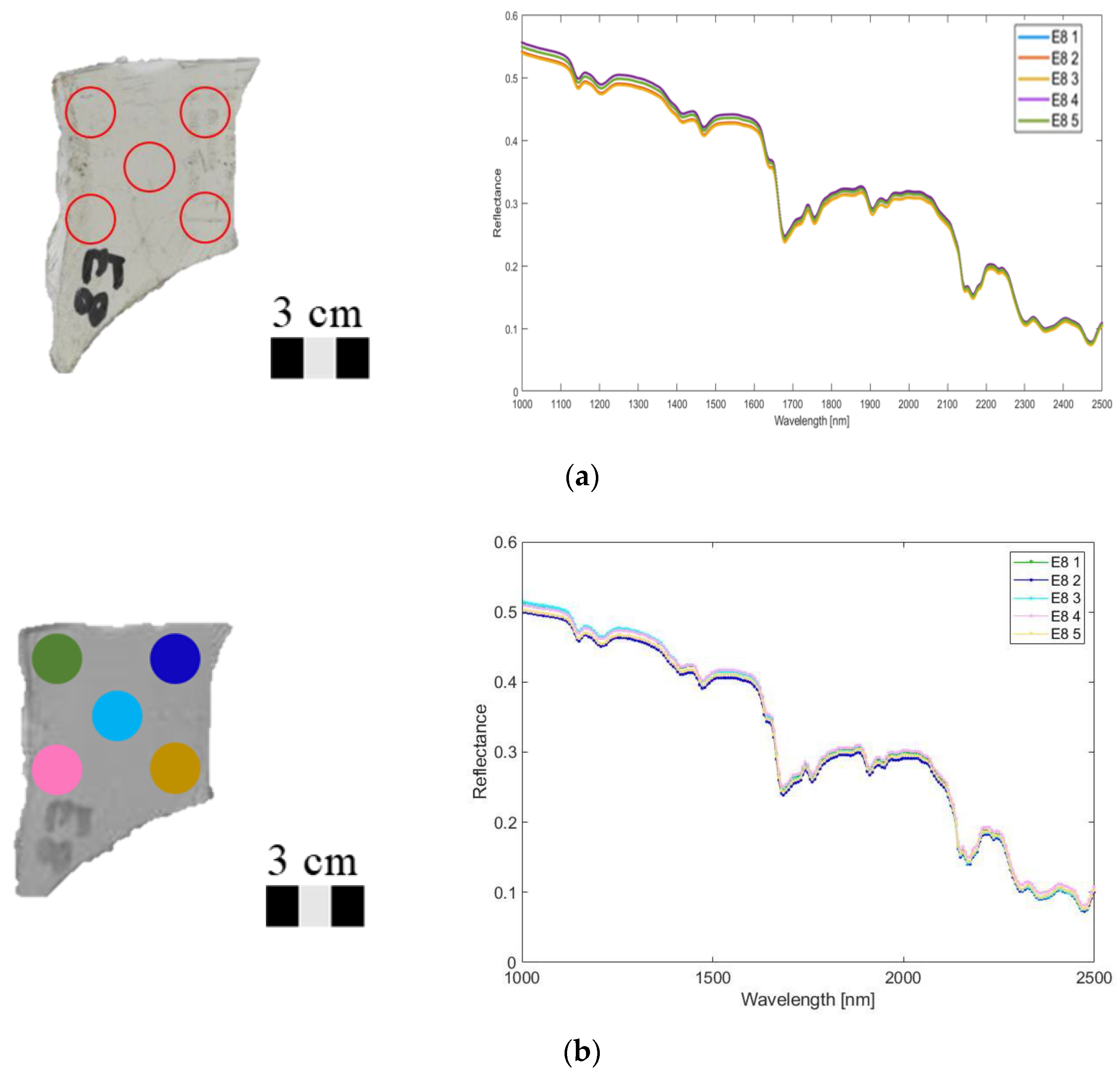
Acquired plastic scraps were divided into two classes according to the recommended Br concentration limits [22]: “High Br content” (>2000 mg/kg) and “Low Br content” (<2000 mg/kg), based on XRF analysis. For each plastic scrap, 5 “single spot based” spectra acquisitions in reflectance mode were carried out using the ASD FieldSpec® device. On the same areas, the average reflectance spectra measured on circular regions of interest (ROIs) of about 10 mm diameter were extracted from the hyperspectral images (Figure 4). The ROIs diameter was established in respect of the average area investigated by the spectroradiometer probe. The average reflectance spectrum of each ROI was compared with the corresponding spectrum measured by the single-point device.
Data pretreatments and exploratory analysis. In spectroscopic applications, spectral preprocessing was not only used to reduce instrument noise, scattering, and other physical phenomena linked to spectra acquisition but also to enhance sample differences and for better solving information in the spectral domains [44]. Scale differences in spectra were mainly due to scattering phenomena and changing environmental conditions affecting illuminants or detectors.
Different preprocessing algorithms were sequentially applied to the acquired reflectance spectra collected by both instruments to enhance differences between the two classes of products according to the bromine contents. In more detail, the Standard Normal Variate (SNV) algorithm was used for reducing scattering effects [45], Savitzky–Golay (S–G) first derivative was used to enhance signal differences [46], Detrend was applied to remove the mean offset from each spectrum [45] and, finally, Mean Center (MC) was used to center columns to have zero mean. Furthermore, spectra were also preprocessed, in order to highlight polymer spectral signatures (i.e., ABS or PS), using SNV, Detrend, and MC.
Principal Component Analysis (PCA) was then carried out in order to evaluate and detect outliers. PCA is a well-known chemometric technique used as a data exploratory tool, that is able to extract the dominants patterns of a spectral data matrix in terms of the product of two smaller matrices of scores and loadings [47,48].
PLS-DA classification models. Partial Least Square Discriminant Analysis (PLS-DA), a supervised technique for pattern recognition, was used to classify the sample data according to bromine content and polymer type. PLS-DA is essentially an inverse-least square approach to the Linear Discriminant Analysis (LDA). The Partial Least Square (PLS) regression was used in this technique to develop a model able to predict the class number for each investigated sample [49,50,51].
For each device, classification models were developed in order to perform discrimination based on bromine content first and then to identify the polymer type.
Classification models for bromine content. As shown in Figure 3, the PLS-DA method was used in order to discriminate “High Br content” and “Low Br content” classes in the 1000–2500 nm spectral range by using the portable spectrophotoradiometer and the HSI benchtop system.
Two classification models were set up: one for the spectra collected by the ASD FieldSpec® 4 Standard-Res and the other for those acquired by the SisuCHEMA XL™. For these models, about 72% of the spectral data was used as the training set, whereas the remaining percentage (28%) was used as the validation set. In more detail, 26 samples were selected to be included in the training set and 10 individuals for the validation set. Venetian Blinds (VB) was used as a cross-validation method for assessing the optimal complexity of the models and choosing the number of Latent Variables (LVs). In this case, 3 LVs were chosen for both models.
The PLS-DA model built from FieldSpec data was applied to the reflectance spectra collected on the validation set samples (10 plastic scraps).
The built PLS-DA of the SisuCHEMA XL™ system spectral data was first applied to the average spectra of the ROIs selected on the validation image (“average spectra”) and then to the validation image (“imaging”—validation set) and the global set (“imaging”).
Classification models for polymer identification. A similar procedure, as described in the previous paragraph, was followed in order to set up the PLS-DA models for polymer classification (Figure 3). The classification models were built using reference spectra of ABS and PS for training and were validated on all samples (global set) for both the sensing devices. In more detail, the PLS-DA model was applied to the spectra collected from the global set by the portable spectrophotoradiometer and, concerning HSI, to the average spectra of the ROIs extracted from the validation set image and to the whole global set image (“imaging”). Four LVs were chosen for both models.
Classification performance assessment. The confusion matrix was considered to evaluate classifier performance coupled with the commonly used performance metrics, that is, Sensitivity, Specificity, Precision, Accuracy, and Class Error [33,52,53]. Sensitivity estimates the model’s ability to avoid false negatives. On the contrary, Specificity is used to evaluate the model’s ability to avoid false positives. Precision, also called positive predictive value, is defined as the ratio between the number of true positives and the number of positives calls. Accuracy is the proportion of correct predictions (both true positives and true negatives) among the total number of cases examined. Those parameters assume values between 0 and 1, where 1 is the ideal value for the model. Finally, Class Error is defined as the misclassified global fraction of particles.
In an object-based logic, the performance of each classification model was computed in terms of Recognition/Accuracy (i.e., the ratio of the well-recognized samples on the total number of samples) and Error (i.e., number of misrecognized samples in respect of the total number of samples) [53,54]. An object was deemed correctly classified when: (i) for punctual spectra acquisitions, more than 3 out of 5 spectra were correctly assigned to their belonging classes and (ii) adopting a hyperspectral approach, 50% or more of the pixels were correctly assigned to their respective classes.
3. Results and Discussion
3.1. X-ray Fluorescence Analysis
Bromine concentrations obtained by XRF of plastic scraps are reported in Table 3. The analyses showed 27 samples (75%) were characterized by a Br content higher than 2000 mg/kg and 9 (25%) by Br content lower than 2000 mg/kg.
3.2. SWIR Spectral Analysis
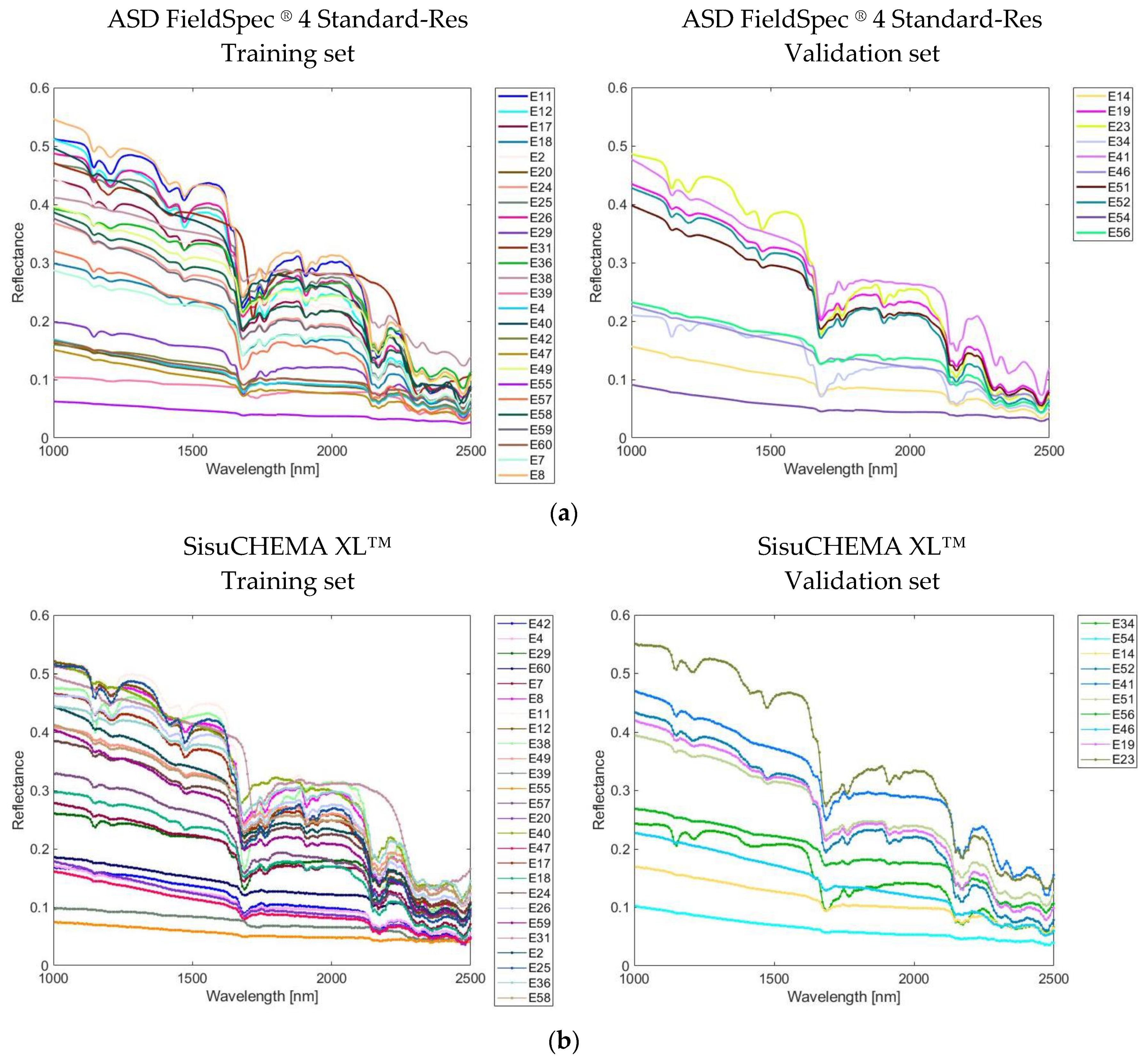
Exploratory analysis. Figure 4 shows an example of the strategy adopted to perform the five punctual acquisitions by the ASD FieldSpec® 4 Standard-Res and the reflectance spectra acquired by the SisuCHEMA XL™ HSI system in the five corresponding ROIs. Figure 5 shows the raw reflectance spectra in the SWIR range (1000–2500 nm), included in the training and validation datasets, for the two devices.
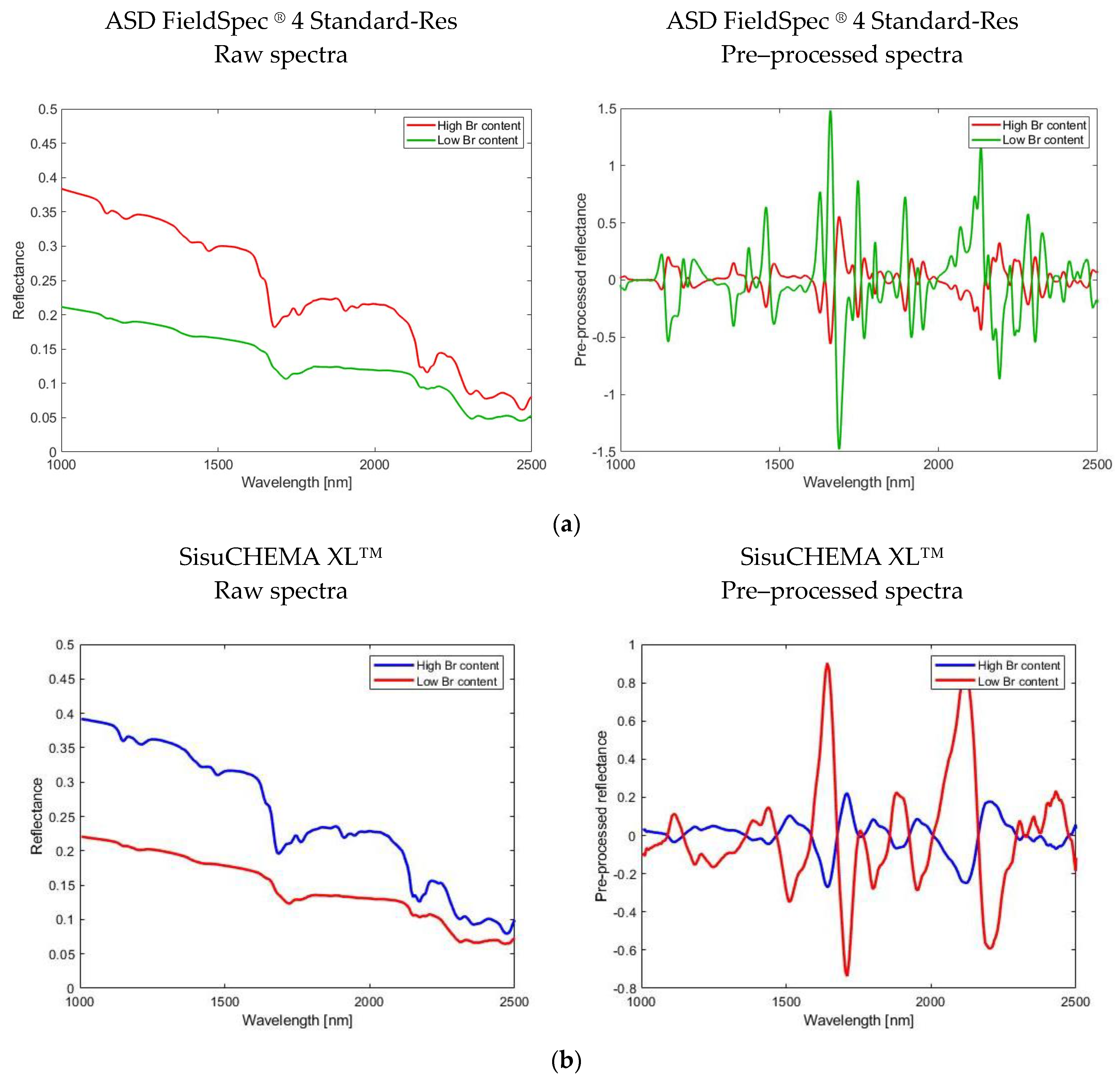
Spectral signature analysis for bromine content assessment. The raw reflectance spectra of the samples averaged according to the two bromine classes (high and low content), collected with the two devices, were preprocessed utilizing the same algorithms in order to correctly compare the further classification results (Figure 6).
The raw reflectance spectra of samples characterized by a high Br content, differently from those characterized by a low Br content, show an extra absorption peak around 1469 nm. This peak can be linked to the presence of TBBPA (tetrabromobisphenol A), as reported in past studies [36,37,40]. Spectra preprocessing enhances the differences among the two classes. As it can be seen in Figure 6, the higher spectral resolution of ASD FieldSpec® 4 Standard-Res produced a more enhanced preprocessed spectrum.
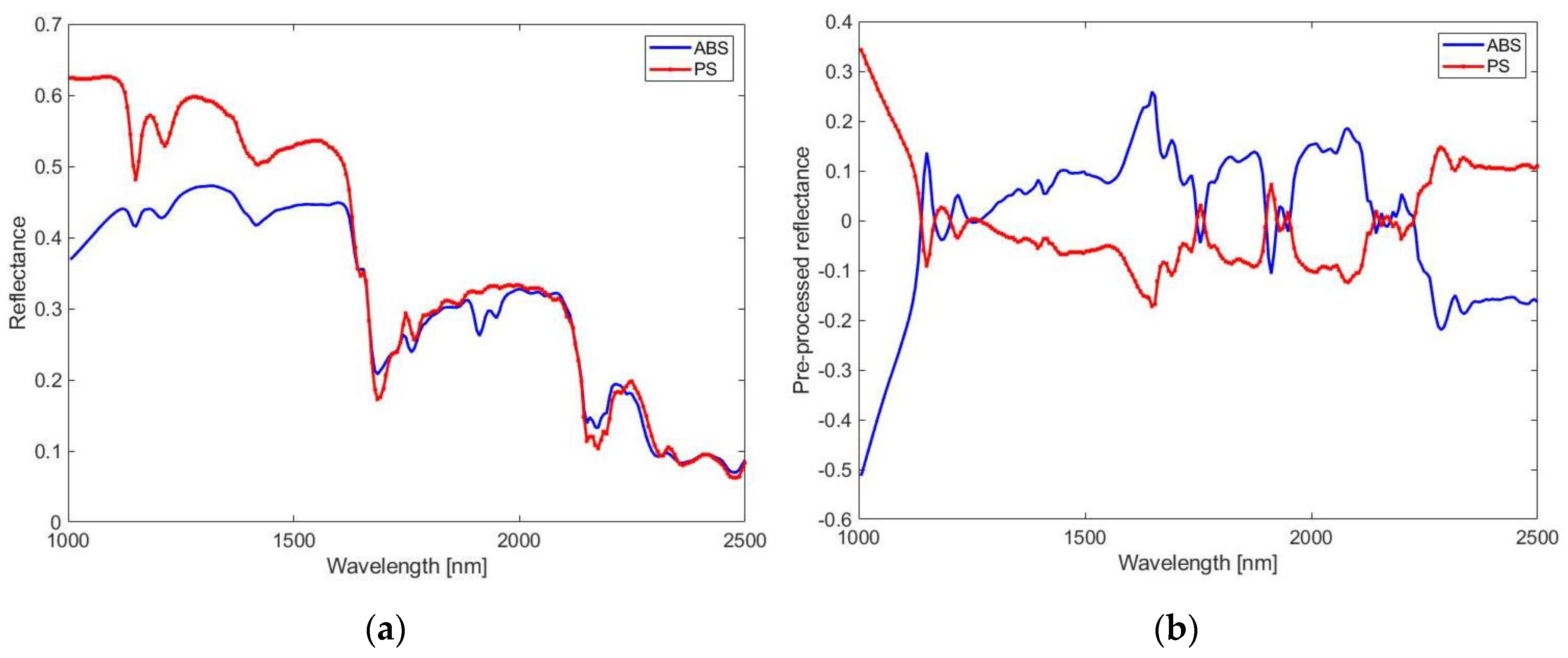
Spectra signature analysis for polymers identification.Figure 7 shows the raw and preprocessed reflectance spectra of the reference polymers used to train the classification model for plastic-type classification (i.e., ABS and PS).
The SWIR range is very useful to identify different polymers because it provides information on the overtone bands of the fundamental groups containing O–H, C–H, N–H, and C–O bonds [55]. In this specific range, the identification of plastics is mainly based on the stretching vibration modes of CH, CH2, and CH3 groups between about 1100 and 1250 nm, corresponding to the 2nd overtone, the 1st overtone ranging from 1650 to 1700 nm, and the combination bands. More in detail, the spectra of PS samples were characterized by absorptions in the 3rd region of harmonics (1043, 1151, 1214, and 1308 nm) due to absorption of C–H2 and C–H, in the second harmonic region (1352, 1415, and 1648 nm) of C–H2 and δC–H2, and in the 1st combination region (1817, 1868, 1918, 2012, and 2074 nm) of C–H group [56]. ABS spectrum had a similar fingerprint to that of PS; the main differences are related to less intensity absorptions of ABS with respect to PS in the 3rd region of harmonics and a different absorption in the 1st combination region (1817, 1868, and 1918 nm) of C–H group.
Classification models for bromine content. Both the built PLS-DA models based on the collected spectra carried out by “single spot” and ROIs based analysis showed good performance in discriminating the bromine content classes as reported in Table 4 and Table 5, respectively, in calibration, cross-validation, and prediction. However, some spectra were incorrectly classified (please refer to Supplementary Materials for details).
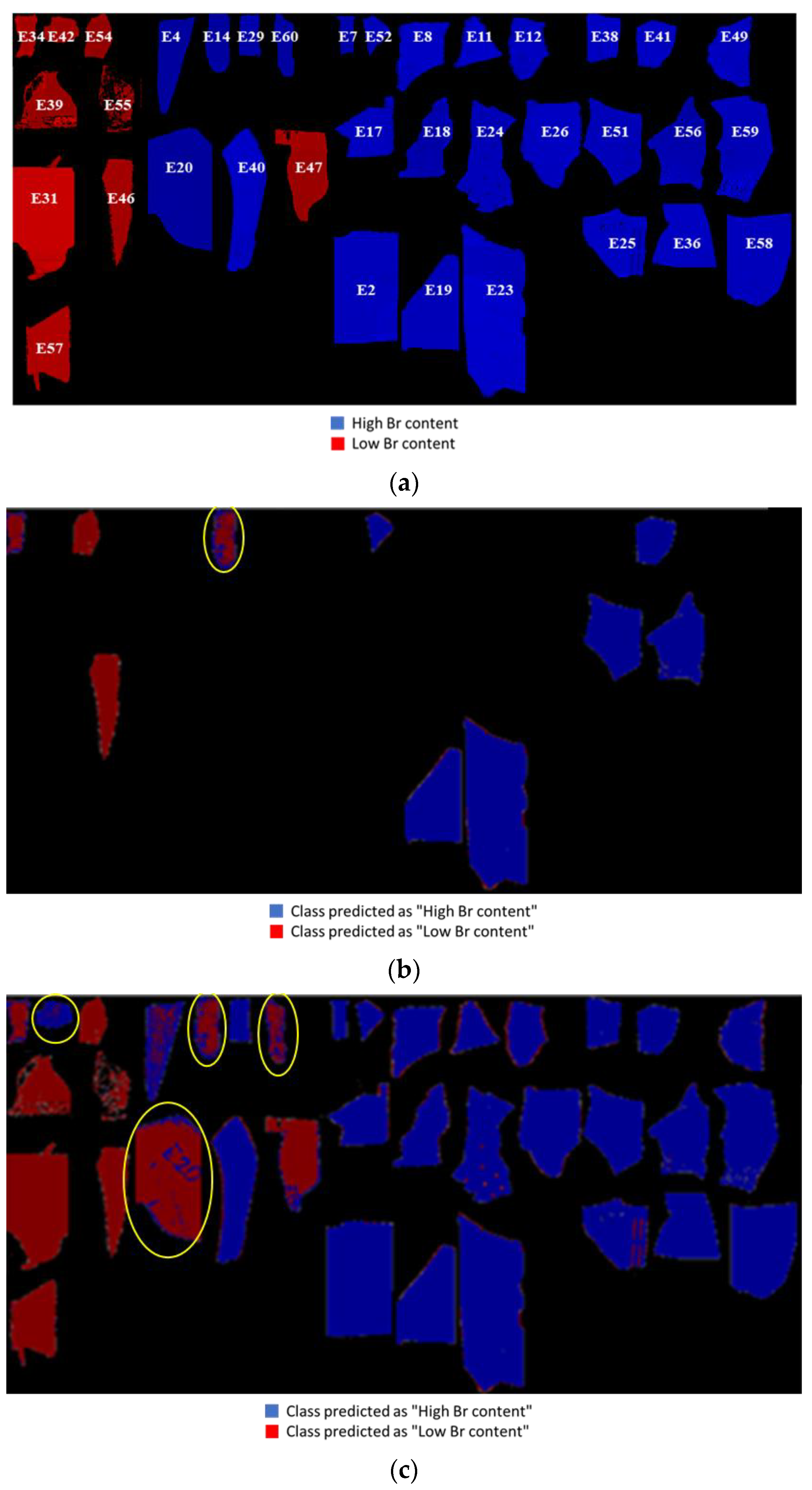
In the case of ASD FieldSpec® 4 Standard-Res data (Table 4), during the calibration phase, Sensitivity and Specificity values were 0.833 and 1.000 for “High Br content” and 1.000 and 0.833 for “Low Br content”, respectively. As shown in Figures S1 and S2, three plastic scraps were not correctly assigned to their real classes (E4, E20, and E60). In the prediction phase, Sensitivity and Specificity values were 0.857 and 1.000 for “High Br content” and 1.000 and 0.857 for “Low Br content”. In this case, sample E14 was misclassified as a “Low Br content” scrap in prediction. Concerning the performance parameters related to SisuCHEMA XL™ average spectral data (Table 5), during the calibration phase Sensitivity and Specificity values were 0.900 and 0.833 for “High Br content” and 0.833 and 0.900 for “Low Br content”, respectively. Sample E20, E42, and E60 were not correctly assigned to their real class. The built classification model, in prediction, confirmed the good performance achieved in calibration (Sensitivity = 0.886, Specificity = 1.000 for “High Br content” and Sensitivity = 1.000, Specificity = 0.886 for “Low Br content”). In this case, the model did not recognize sample E14 as a “High Br content” one. Finally, the performance parameters related to the PLS-DA classification of the validation image set and global image set are reported in Table 5. For the validation set, the results showed that all the samples, except E14, were correctly classified (Sensitivity = 0.950, Specificity = 0.951 for “High Br content” and Sensitivity = 0.951, Specificity = 0.950 for “Low Br content”). For the global set, the performance parameters showed also in this case good values (Sensitivity = 0.881, Specificity = 0.932 for “High Br content” and Sensitivity = 0.932, Specificity = 0.881 for “Low Br content”), with four samples incorrectly classified: E42, E14, E60, and E20. With reference to the latter case, the classification results are also presented in terms of prediction maps in Figure 8, for both validation image set and global image set, together with the false-color image, indicating the true class membership, highlighting the few misclassified fragments. All the misclassified samples show flat spectra with low reflectance intensities, as can be seen in Figure 5 and Figure S3 (between 0.16–0.2).
The results (Table 4 and Table 5) showed similar performances between the ASD FieldSpec® 4 Standard Res-based approach compared to the SisuCHEMA XL™ one. In calibration and cross-validation phases, performance metrics obtained using the spectrophotoradiometer data were better than those obtained by the HSI system data. On the contrary, the performances obtained in prediction were slightly better for the classification performed by HSI system data than the portable system, since the Sensitivity and Specificity, as well as Precision and Accuracy, were higher for both classes.
Results obtained in prediction for the validation image set and global image confirm the reliability of the built model.
Classification models for polymer identification. The classification performance metrics were obtained following three different approaches: the first two based on the global set referred to ASD FieldSpec® 4 Standard-Res and SisuCHEMA XL™ spectra and the third based on SisuCHEMA XL™ hyperspectral images mosaic (Table 6).
The classification model applied to ASD FieldSpec® 4 Standard-Res data was not able to correctly classify seven samples (E29, E31, E38, E39, E40, E46, and E55): six PS individuals were incorrectly classified as ABS and one ABS as PS. This fact was confirmed from Sensitivity and Specificity values (Sensitivity = 0.950, Specificity = 0.638 for ABS and Sensitivity = 0.638, Specificity = 0.950 for PS), reported in Table 6.
The classification model based on the analysis of SisuCHEMA XL™ global set spectra was not able to classify four PS samples (E31, E39, E46, and E57) that were incorrectly classified as ABS (Sensitivity = 1.000, Specificity = 0.713 for ABS and Sensitivity = 0.713, Specificity = 1.000 for PS).
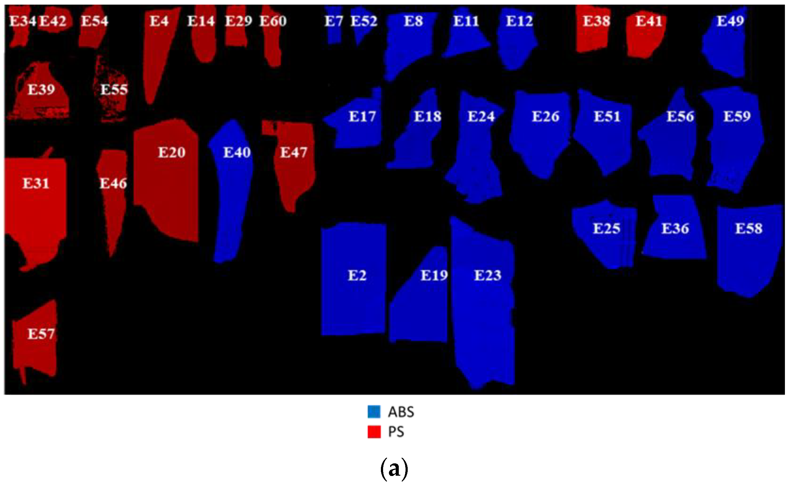
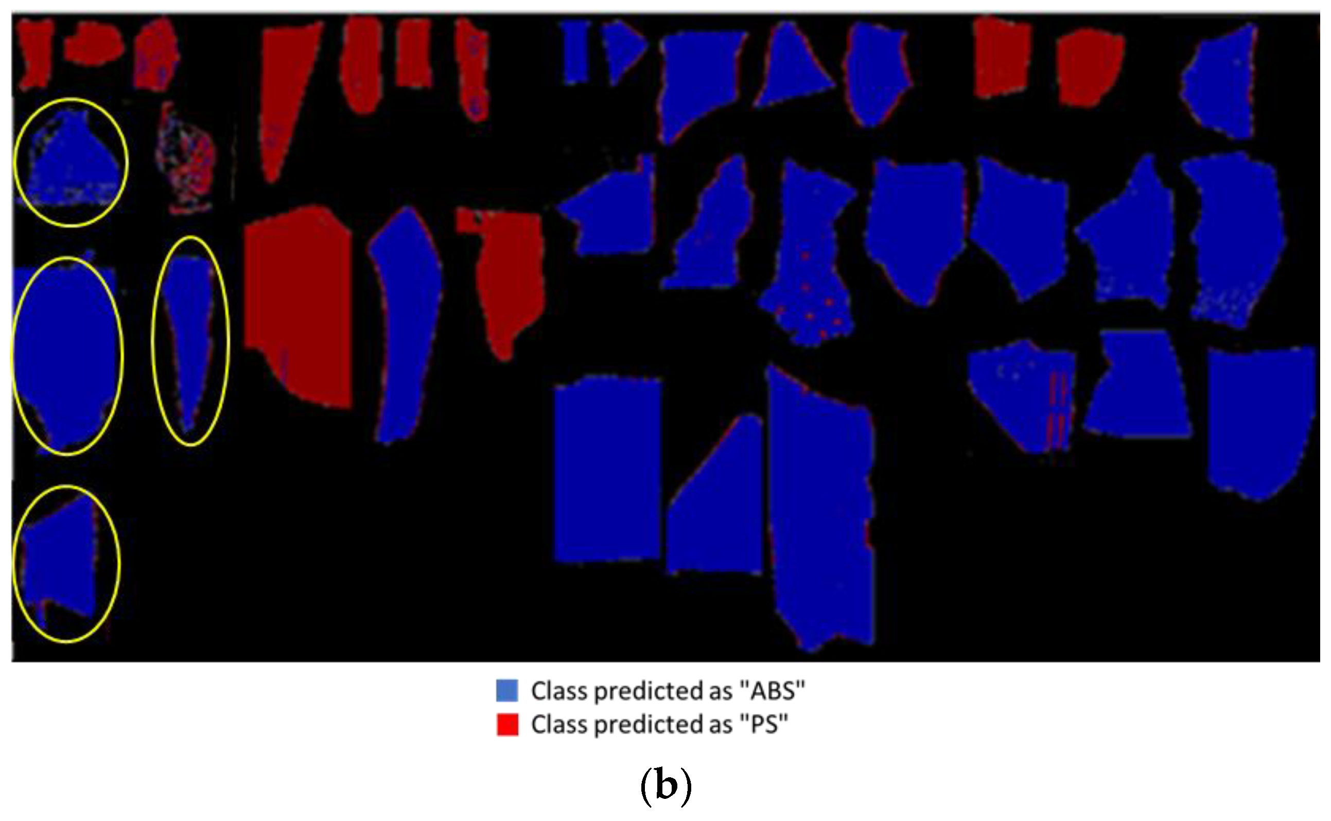
A similar performance was achieved by applying the classification model based on hyperspectral images mosaic global set. The prediction map resulting from the PLS-DA is shown in Figure 9, together with the false-color image, indicating the true class membership (Figure 9a). As can be seen in Figure 9b, PS samples (E31, E39, E46, and E57) were incorrectly classified as ABS (Sensitivity = 0.985, Specificity = 0.682 for ABS and Sensitivity = 0.682, Specificity = 0.985 for PS).
The observed misclassification in discriminating ABS and PS was also observed by other authors. Wu et al. (2020) reported that only 72.8% of PS was correctly classified, and the remaining percentage was misclassified as ABS in PLS-DA classification using NIR spectroscopy (900–1700 nm). Similar results were also achieved by Amigo et al. (2015) using this approach. In this latter case, a large number of pixels were not correctly assigned to the real polymer class [33].
Overall classification models performances. Overall classification performances of the set-up models are reported in Table 7. The set-up models to discriminate Br classes with FieldSpec and SisuCHEMA spectral data achieved a Recognition of 88.46% and 90.00% for the training and validation set, respectively. The models performed to identify the type of polymer achieved a Recognition of 80.56% and 88.89% for FieldSpec data and SisuCHEMA (global set), respectively.
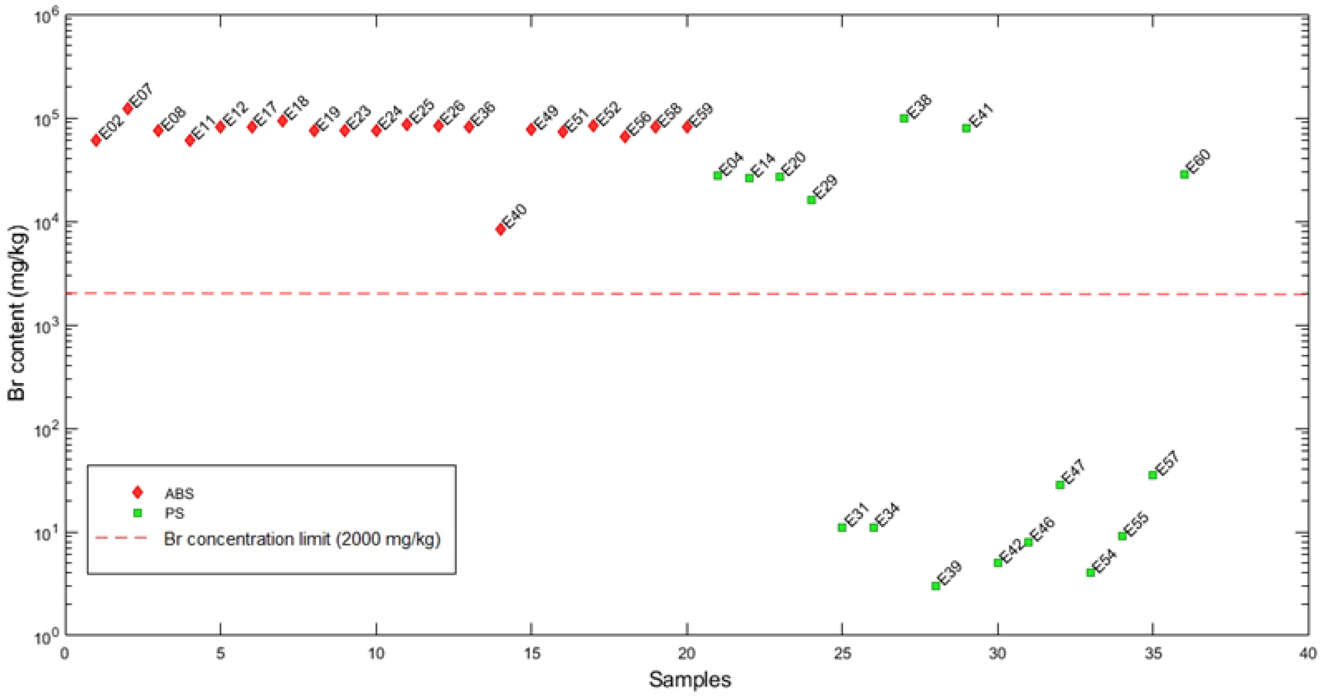
Combining bromine content measured by XRF and polymer type of the single scrap (Figure 10), it can be seen that all individual objects identified as ABS (n = 20; Br content = 76,378 ± 20,593 mg/kg) exceeded the bromine content regulation limit of 2000 mg/kg. On the contrary, only 47% of PS scraps exceeded the Br content regulation limit (n = 16; Br content = 19,001 ± 30,015 mg/kg). As seen from the HSI-based classification for bromine content, the misclassified samples were PS plastic scraps (Figure 8 and Figure 9). The misclassification mainly occurred for PS with low Br content, which was incorrectly assigned to the “high Br class”.
4. Conclusions and Future Perspectives
This study was carried out in order to test the predictive ability of SWIR working instruments to discriminate plastic scraps with high bromine content from the low ones. This goal was achieved using two different equipment: a portable spectrophotoradiometer and a benchtop HSI system. The set-up models to discriminate bromine content classes with the portable spectrophotoradiometer and HSI data achieved equal Recognition (i.e., 88.46% and 90% for the training and validation set, respectively). The models performed to identify the type of polymer achieved a Recognition of 80.56% and 88.89% for FieldSpec and SisuCHEMA data (global sets), respectively. Both the instrumentations gave useful information about BFRs added polymer scraps, for example, to evaluate the performances of the currently adopted density separation process for brominated plastics in recycling plants, especially when dealing with different polymers characterized by similar densities, such as ABS and PS.
Both the instrumentations gave useful information about BFRs added polymer scraps, for example, to evaluate the performances of the currently adopted density separation process for brominated plastics in recycling plants, especially when dealing with different polymers characterized by similar densities, such as ABS and PS. The utilization of the portable instrument could be applied to a rapid test on samples collected at the entrance (i.e., feed) and/or on the process streams moving towards the exit and/or on the recovered product of a waste treatment plant. In addition, SWIR-HSI system can be utilized not only for the same above-mentioned purposes but also as a core engine to implement online sorting logics.
The proposed approach—if systematically applied at the recycling plant scale—could quickly, non-destructively, and efficiently carry out a complete control of brominated plastic contaminants. In fact, this method can both identify the bromine content of WEEE plastics and assess the polymer type.
Both methodologies can be seen as a tool to maximize the recyclable polymer fractions, removing those individuals containing toxic substances (i.e., Br), thus increasing the circular use of materials, reducing pollution, toxic emissions, landfill, and also contributing to mitigate climate change effects, specifically addressing the principles of circular economy and the Sustainable Development Goals (SDGs), as SDG 9 (Industry, Innovation, and Infrastructure), SDG 12 (Responsible Consumption and Production (SDG 12), SDG 13 (Climate Action), SDG 14 (Life Below Water), and SDG 15 (Life on Land).
Supplementary Materials
The following are available online at https://0-www-mdpi-com.brum.beds.ac.uk/article/10.3390/recycling6030054/s1, Figure S1: Class prediction most probable vs. individual spectra for ASD FieldSpec® 4 Standard Res and SisuCHEMA XL™, Figure S2: Misclassified spectra vs. individual spectra for ASD FieldSpec® 4 Standard Res and SisuCHEMA XL™, Figure S3: Misclassified spectra for ASD FieldSpec® 4 Standard Res (a) and SisuCHEMA XL™.
Author Contributions
Conceptualization, G.B., S.S. and P.H.; methodology, L.F. and R.G.; software, L.F. and R.G.; validation, G.B., L.F., R.G., P.H. and S.S.; formal analysis, L.F., R.G. and P.H.; investigation, G.B., L.F., R.G., P.H. and S.S.; resources, G.B., S.S. and P.H.; data curation, L.F., R.G. and P.H.; writing—original draft preparation, L.F. and R.G.; writing—review and editing, G.B., P.H. and S.S.; visualization, G.B. and S.S.; supervision, G.B. and S.S. All authors have read and agreed to the published version of the manuscript.
Funding
This research received no external funding.
Institutional Review Board Statement
Not applicable.
Informed Consent Statement
Not applicable.
Data Availability Statement
The data presented in this study are available on request from the corresponding authors.
Acknowledgments
The authors wish to thank Galloo Plastics SA (Halluin, France) for having provided all the samples utilized in this study and for the profitable discussions.
Conflicts of Interest
The authors declare no conflict of interest.
References
- Zeng, X.; Mathews, J.A.; Li, J. Urban Mining of E-Waste is Becoming More Cost-Effective than Virgin Mining. Environ. Sci. Technol. 2018, 52, 4835–4841. [Google Scholar] [CrossRef]
- Robinson, B.H. E-waste: An assessment of global production and environmental impacts. Sci. Total Environ. 2009, 408, 183–191. [Google Scholar] [CrossRef] [PubMed]
- Álvarez-De-Los-Mozos, E.; Rentería-Bilbao, A.; Díaz-Martín, F. WEEE Recycling and Circular Economy Assisted by Collaborative Robots. Appl. Sci. 2020, 10, 4800. [Google Scholar] [CrossRef]
- Grigore, M.E. Methods of recycling, properties and applications of recycled thermoplastic polymers. Recycling 2017, 2, 24. [Google Scholar] [CrossRef] [Green Version]
- PlasticsEurope. Plastics—The Facts 2020. Available online: https://www.plasticseurope.org/it/resources/publications/4312-plastics-facts-2020 (accessed on 26 July 2021).
- Haarman, A.; Magalini, F.; Courtois, J. Study on the Impacts of Brominated Flame Retardants on the Recycling of WEEE Plastics in Europe. Report by Sofies Group. 2020. Available online: https://www.bsef.com/news/sofiesreport/ (accessed on 16 August 2021).
- Grigorescu, R.M.; Grigore, M.D.; Iancu, L.; Ghioca, P.; Ion, R.-M. Waste Electrical and Electronic Equipment: A Review on the Identification Methods for Polymeric Materials. Recycling 2019, 4, 32. [Google Scholar] [CrossRef] [Green Version]
- Tostar, S.; Stenvall, E.; Foreman, M.R.S.J.; Boldizar, A. The Influence of Compatibilizer Addition and Gamma Irradiation on Mechanical and Rheological Properties of a Recycled WEEE Plastics Blend. Recycling 2016, 1, 101–110. [Google Scholar] [CrossRef] [Green Version]
- Esposito, L.; Cafiero, L.; De Angelis, D.; Tuffi, R.; Ciprioti, S.V. Valorization of the plastic residue from a WEEE treatment plant by pyrolysis. Waste Manag. 2020, 112, 1–10. [Google Scholar] [CrossRef] [PubMed]
- Makenji, K.; Savage, M. Mechanical methods of recycling plastics from WEEE. In Waste Electrical and Electronic Equipment (WEEE) Handbook; Goodship, V., Stevels, A., Eds.; Woodhead Publishing Limited: Cambridge, UK, 2012; pp. 212–238. [Google Scholar] [CrossRef]
- Gill, R.; Hurley, S.; Brown, R.; Tarrant, D.; Dhaliwal, J.; Sarala, R.; Park, J.-S.; Patton, S.; Petreas, M. Polybrominated Diphenyl Ether and Organophosphate Flame Retardants in Canadian Fire Station Dust. Chemosphere 2020, 253, 126669. [Google Scholar] [CrossRef] [PubMed]
- Huisman, J.; Magalini, F.; Kuehr, R.; Maurer, C.; Ogilvie, S.; Poll, J. Review of Directive 2002/96 on Waste Electrical and Electronic Equipment (WEEE); United Nations University: Bonn, Germany, 2008. [Google Scholar]
- Hennebert, P.; Filella, M. WEEE plastic sorting for bromine essential to enforce EU regulation. Waste Manag. 2018, 71, 390–399. [Google Scholar] [CrossRef]
- Tohka, A.; Zevenhove, R. Brominated flame retardants—Brominated flame retardants A nuisance in thermal waste processing? In TMS 2002 Extraction and Processing Division Meeting on Recycling and Waste Treatment in Mineral and Metal Processing; Luleå University of Technology: Luleå, Sweden, 2002; Volume 2, pp. 753–763. [Google Scholar]
- Gómez, M.; Peisino, L.E.; Kreiker, J.; Gaggino, R.; Cappelletti, A.L.; Martín, S.E.; Uberman, P.M.; Positieri, M.; Raggiotti, B.B. Stabilization of hazardous compounds from WEEE plastic: Development of a novel core-shell recycled plastic aggregate for use in building materials. Constr. Build. Mater. 2019, 230, 116977. [Google Scholar] [CrossRef]
- Malliari, E.; Kalantzi, O.-I. Children’s exposure to brominated flame retardants in indoor environments—A review. Environ. Int. 2017, 108, 146–169. [Google Scholar] [CrossRef] [PubMed]
- Official Journal of the European Union. EC 2002. Directive 2002/95/EC of the European Parliament and of the Council of 27 January 2003. The Restriction of the Use of Certain Hazardous Substances in Electrical and Electronic Equipment 2002. Available online: https://eur–lex.europa.eu/LexUriServ/LexUriServ.do?uri=OJ:L:2003:037:0019:0023:EN:PDF (accessed on 29 April 2020).
- Publications Office of the European Union. Directive 2011/65/Eu of the European Parliament and of the Council of 8 June 2011 on the Restriction of the Use of Certain Hazardous Substances in ELECTRICAL and electronic Equipment; Publications Office of the European Union: Luxembourg, 2012; Volume 54, pp. 88–110. [Google Scholar] [CrossRef]
- Puype, F.; Samsonek, J.; Knoop, J.; Egelkraut-Holtus, M.; Ortlieb, M. Evidence of waste electrical and electronic equipment (WEEE) relevant substances in polymeric food-contact articles sold on the European market. Food Addit. Contam. Part A 2015, 32, 410–426. [Google Scholar] [CrossRef]
- Samsonek, J.; Puype, F. Occurrence of brominated flame retardants in black thermo cups and selected kitchen utensils purchased on the European market. Food Addit. Contam. Part A 2013, 30, 1976–1986. [Google Scholar] [CrossRef]
- Schecter, A.; Szabo, D.T.; Miller, J.; Gent, T.L.; Malik-Bass, N.; Petersen, M.; Paepke, O.; Colacino, J.A.; Hynan, L.S.; Harris, T.R.; et al. Hexabromocyclododecane (HBCD) Stereoisomers in U.S. Food from Dallas, Texas. Environ. Health Perspect. 2012, 120, 1260–1264. [Google Scholar] [CrossRef] [PubMed] [Green Version]
- European Committee for Electrotechnical Standardization. CLC/TS 50625–3–1. Requirements for Collection, Logistics and Processing for Waste Electrical and Electronic Equipment (WEEE)—Part 3–1: Specifications for Depollution; CENELEC: Brussels, Belgium, 2015. [Google Scholar]
- Adam, A.M.; Altalhi, T.A.; El-Megharbel, S.M.; Saad, H.A.; Refat, M.S. Using a Modified Polyamidoamine Fluorescent Dendrimer for Capturing Environment Polluting Metal Ions Zn2+, Cd2+, and Hg2+: Synthesis and Characterizations. Crystals 2021, 11, 92. [Google Scholar] [CrossRef]
- Fh–ICT. High Quality Plastic Materials from Electronic Wastes by use of Combined Identification Methods and New Handling Technologies. In COMBIDENT Final Technical Report, EU Contract No BRPR–CT98–0778, UNDERTAKEN by the Fraunhofer; Institut für Chemische Technologie: Pfinztal, Germany, 2001. [Google Scholar]
- Bonifazi, G.; Capobianco, G.; Palmieri, R.; Serranti, S. Hyperspectral imaging applied to the waste recycling sector. Spectrosc. Eur. 2019, 31, 8–11. [Google Scholar]
- Bonifazi, G.; Gasbarrone, R.; Serranti, S. Near InfraRed–based hyperspectral imaging approach for secondary raw materials processing in solid waste sector. In Proceedings of the UBT International Conference, Pristina, Kosovo, 25–27 October 2019; ISBN 978-9951-550-19-2. [Google Scholar] [CrossRef]
- Geladi, P.; Grahn, H.; Burger, J. Multivariate Images, Hyperspectral Imaging: Background and equipment. In Techniques and Applications of Hyperspectral Image Analysis; Grahn, H., Geladi, P., Eds.; John Wiley & Sons: West Sussex, UK, 2007; pp. 1–15. [Google Scholar]
- Bonifazi, G.; Gasbarrone, R.; Serranti, S. Characterization of printed circuit boards from e–waste by products for copper beneficiation. In Proceedings of the ECOMONDO 2018, Rimini, Italy, 6–9 November 2018; pp. 65–69. [Google Scholar]
- Bonifazi, G.; Gasbarrone, R.; Palmieri, R.; Serranti, S. Plastic identification from end of life flat monitors by hyperspectral imaging methods. In Proceedings of the Sardinia 2019: 17th International Waste Management and Landfill Symposium, Forte Village, Cagliari, Italy, 30 September–4 October 2019. [Google Scholar]
- Bonifazi, G.; Gasbarrone, R.; Palmieri, R.; Serranti, S. Near infrared hyperspectral imaging-based approach for end-of-life flat monitors recycling. Automatisierungstechnik 2020, 68, 265–276. [Google Scholar] [CrossRef]
- Bonifazi, G.; Fiore, L.; Hennebert, P.; Serranti, S. An Efficient Strategy Based on Hyperspectral Imaging for Brominated Plastic Waste Sorting in a Circular Economy Perspective. In Advances in Polymer Processing; Hopmann, C., Dahlmann, R., Eds.; Springer Nature: Basingstoke, UK, 2020; pp. 14–27. [Google Scholar] [CrossRef]
- Palmieri, R.; Bonifazi, G.; Serranti, S. Recycling–oriented characterization of plastic frames and printed circuit boards from mobile phones by electronic and chemical imaging. Waste Manag. 2014, 34, 2120–2130. [Google Scholar] [CrossRef]
- Amigo, J.M.; Babamoradi, H.; Elcoroaristizabal, S. Hyperspectral image analysis. A tutorial. Anal. Chim. Acta 2015, 896, 34–51. [Google Scholar] [CrossRef] [PubMed]
- Bonifazi, G.; Capobianco, G.; Serranti, S. A hierarchical classification approach for recognition of low-density (LDPE) and high-density polyethylene (HDPE) in mixed plastic waste based on short-wave infrared (SWIR) hyperspectral imaging. Spectrochim. Acta Part A Mol. Biomol. Spectrosc. 2018, 198, 115–122. [Google Scholar] [CrossRef]
- Caballero, D.; Bevilacqua, M.; Amigo, J.M. Application of hyperspectral imaging and chemometrics for classifying plastics with brominated flame retardants. J. Spectr. Imaging 2019, 8, 1–16. [Google Scholar] [CrossRef] [Green Version]
- Leitner, R.; Mcgunnigle, G.; Kraft, M.; De Biasio, M.; Rehrmann, V.; Balthasar, D. Real-time detection of flame-retardant additives in polymers and polymer blends with NIR imaging spectroscopy.Advanced Environmental, Chemical, and Biological Sensing Technologies VI. Proc. SPIE 2009, 7312, 73120. [Google Scholar] [CrossRef]
- Schlummer, M. Recycling of Postindustrial and Postconsumer Plastics Containing Flame Retardants. In Polymer Green Flame Retardants; Elsevier: Amsterdam, The Netherlands, 2014; pp. 869–889. [Google Scholar] [CrossRef]
- Serranti, S.; Luciani, V.; Bonifazi, G.; Hu, B.; Rem, P.C. An innovative recycling process to obtain pure polyethylene and polypropylene from household waste. Waste Manag. 2015, 35, 12–20. [Google Scholar] [CrossRef] [PubMed]
- Serranti, S.; Fiore, L.; Bonifazi, G.; Takeshima, A.; Takeuchi, H.; Kashiwada, S. Microplastics characterization by hyperspectral imaging in the SWIR range. Proc. SPIE 2019, 11197, 1119710. [Google Scholar] [CrossRef]
- Wu, X.; Li, J.; Yao, L.; Xu, Z. Auto-sorting commonly recovered plastics from waste household appliances and electronics using near-infrared spectroscopy. J. Clean. Prod. 2020, 246, 118732. [Google Scholar] [CrossRef]
- ASD Inc. FieldSpec® 4 User Manual, ASD Document 600979, Rev. D; ASD Inc.: Falls Church, VA, USA, 2015. [Google Scholar]
- ASD Inc. RS3™ User Manual, ASD Document 600545, Rev. E; ASD Inc.: Falls Church, VA, USA, 2008. [Google Scholar]
- Gasbarrone, R. Gasby90/FieldSpec4_Import3 (v.3.1); Zenodo: Geneva, Switzerland, 2020. [Google Scholar] [CrossRef]
- Rinnan, A.; van den Berg, F.; Engelsen, S.B. Review of the most common pre-processing techniques for near-infrared spectra. TrAC Trends Anal. Chem. 2009, 28, 1201–1222. [Google Scholar] [CrossRef]
- Barnes, R.J.; Dhanoa, M.S.; Lister, S.J. Standard Normal Variate Transformation and De-Trending of Near-Infrared Diffuse Reflectance Spectra. Appl. Spectrosc. 1989, 43, 772–777. [Google Scholar] [CrossRef]
- Savitzky, A.; Golay, M.J.E. Smoothing and Differentiation of Data by Simplified Least Squares Procedures. Anal. Chem. 1964, 36, 1627–1639. [Google Scholar] [CrossRef]
- Beebe, K.R.; Pell, R.J.; Seasholtz, M.B. Chemometrics: A Practical Guide; Wiley–Interscience: Hoboken, NJ, USA, 1998. [Google Scholar]
- Wold, S.; Esbensen, K.; Geladi, P. Principal component analysis. Chemometr. Intell. Lab. 1987, 2, 37–52. [Google Scholar] [CrossRef]
- Barker, M.; Rayens, W. Partial least squares for discrimination. J. Chemom. 2003, 17, 166–173. [Google Scholar] [CrossRef]
- Wise, B.; Gallagher, N.; Bro, R.; Shaver, J.; Windig, W.; Koch, R. Chemometrics Tutorial for PLS_Toolbox and Solo; Eigenvector Research Inc.: Wenatchee, WA, USA, 2006. [Google Scholar]
- Ballabio, D.; Consonni, V. Classification tools in chemistry. Part 1: Linear models. PLS-DA. Anal. Methods 2013, 5, 3790–3798. [Google Scholar] [CrossRef]
- Fawcett, T. An introduction to ROC analysis. Pattern Recognit. Lett. 2005, 27, 861–874. [Google Scholar] [CrossRef]
- Ballabio, D.; Todeschini, R. Multivariate Classification for Qualitative Analysis. In Infrared Spectroscopy for Food Quality Analysis and Control; Elsevier: Amsterdam, The Netherlands, 2009; pp. 83–104. [Google Scholar]
- Silva, E.J.; Britto, A.S.; Oliveira, L.S.; Enembreck, F.; Sabourin, R.; Koerich, A.L. A two–step cascade classification method. In Proceedings of the International Conference on Neural Networks (IJCNN’2017), Anchorage, AK, USA, 14–19 May 2017; pp. 573–580. [Google Scholar]
- Workman, J., Jr.; Weyer, L. Practical Guide and Spectral Atlas for Interpretive Near–Infrared Spectroscopy; CRC Press: Boca Raton, FL, USA, 2012. [Google Scholar]
- Stuart, B. Infrared Spectroscopy: Fundamentals and Applications. In Analytical Techniques in the Sciences (AnTS); John Wiley & Sons: Hoboken, NJ, USA, 2004. [Google Scholar] [CrossRef]
Figure 1.
Conventional recycling process of WEEE plastics (a), possible scenarios for quality control applications by NIR/SWIR portable devices and HSI-NIR/SWIR systems (b), and sorting solutions adopting HSI-NIR/SWIR platform (c). Adapted from Haarman et al. (2020).
Figure 1.
Conventional recycling process of WEEE plastics (a), possible scenarios for quality control applications by NIR/SWIR portable devices and HSI-NIR/SWIR systems (b), and sorting solutions adopting HSI-NIR/SWIR platform (c). Adapted from Haarman et al. (2020).

Figure 2.
Analyzed shredded plastic scraps from CRT monitors and televisions.

Figure 3.
Flow chart adopted to perform the classification procedures for the identification of samples characterized by high and low bromine contents and the further recognition of ABS and PS scraps.
Figure 3.
Flow chart adopted to perform the classification procedures for the identification of samples characterized by high and low bromine contents and the further recognition of ABS and PS scraps.

Figure 4.
Topological assessment strategy, adopted for each plastic scrap, to select the five spectra acquisition points by ASD FieldSpec® 4 Standard-Res and the resulting raw reflectance spectra (1000–2500 nm) (a) and the corresponding five Regions of interest (ROIs) utilized to collect raw reflectance spectra (1000–2500 nm) by the SisuCHEMA XL™ HSI system (b).

Figure 5.
Average raw reflectance spectra (1000–2500 nm) of each plastic scrap collected by ASD FieldSpec® 4 Standard-Res (a) and extracted from ROIs investigated by the SisuCHEMA XL™ (b).
Figure 5.
Average raw reflectance spectra (1000–2500 nm) of each plastic scrap collected by ASD FieldSpec® 4 Standard-Res (a) and extracted from ROIs investigated by the SisuCHEMA XL™ (b).

Figure 6.
Raw and preprocessed reflectance spectra (1000–2500 nm) averaged according to the two groups of samples characterized by high and low bromine content, collected by ASD FieldSpec® 4 Standard-Res (a) and extracted from ROIs investigated by the SisuCHEMA XL™ (b).
Figure 6.
Raw and preprocessed reflectance spectra (1000–2500 nm) averaged according to the two groups of samples characterized by high and low bromine content, collected by ASD FieldSpec® 4 Standard-Res (a) and extracted from ROIs investigated by the SisuCHEMA XL™ (b).

Figure 7.
Average raw reflectance spectra (a) and preprocessed reflectance spectra (b) of the two reference polymer classes (ABS and PS), obtained after ROIs selection on SisuCHEMA XL™ data (wavelength range: 1000–2500 nm).
Figure 7.
Average raw reflectance spectra (a) and preprocessed reflectance spectra (b) of the two reference polymer classes (ABS and PS), obtained after ROIs selection on SisuCHEMA XL™ data (wavelength range: 1000–2500 nm).

Figure 8.
True class membership (a) and most probable class prediction for SisuCHEMA XL™ data obtained after the application of PLS-DA model for the validation set (b) and the global set (c). Blue = “High Br content” class; Red = “Low Br content” class. Samples circled in yellow were incorrectly identified.

Figure 9.
True class membership (a) and class prediction most probable for SisuCHEMA XL™ obtained after the application of the PLS-DA model on the global set hyperspectral images mosaic (b). Blue = “ABS” class; red = “PS” class. Samples circled in yellow were incorrectly identified.
Figure 9.
True class membership (a) and class prediction most probable for SisuCHEMA XL™ obtained after the application of the PLS-DA model on the global set hyperspectral images mosaic (b). Blue = “ABS” class; red = “PS” class. Samples circled in yellow were incorrectly identified.


Figure 10.
Samples labeled according to the plastic type (ABS and PS) versus Br content (mg/kg) plot. Br concentration limit, as reported from CENELEC technical specification (CENELEC CLC/TS 50625–3–1, 2015), is shown as a red slashed line.
Figure 10.
Samples labeled according to the plastic type (ABS and PS) versus Br content (mg/kg) plot. Br concentration limit, as reported from CENELEC technical specification (CENELEC CLC/TS 50625–3–1, 2015), is shown as a red slashed line.


Table 1.
Characteristics of the examined plastic scraps in respect of their physical attributes (color, thickness, and weight).
Table 1.
Characteristics of the examined plastic scraps in respect of their physical attributes (color, thickness, and weight).
| Sample ID | Color | Thickness (mm) | Weight (g) | Sample ID | Color | Thickness (mm) | Weight (g) |
|---|---|---|---|---|---|---|---|
| E2 | White | 3 | 26.26 | E36 | White | 3 | 7.18 |
| E4 | Grey | 2.5 | 4.2 | E38 | White | 3 | 11.45 |
| E7 | Grey | 4 | 5.41 | E39 | Grey | 3 | 5.19 |
| E8 | White | 3 | 5.32 | E40 | White | 3 | 8.75 |
| E11 | White | 4 | 3.33 | E41 | White | 2 | 2.79 |
| E12 | White | 3.5 | 4.18 | E42 | Grey | 3 | 4.7 |
| E14 | Grey | 3 | 10.22 | E46 | White | 2 | 3.18 |
| E17 | White | 3 | 6.66 | E47 | White | 3 | 4.93 |
| E18 | Grey | 3 | 4.63 | E49 | White | 4 | 5.39 |
| E19 | White | 3 | 12.9 | E51 | White | 3 | 8.53 |
| E20 | Grey | 3 | 20.46 | E52 | White | 3 | 4.18 |
| E23 | White | 4 | 35.13 | E54 | Grey | 3 | 7.13 |
| E24 | White | 2 | 8.12 | E55 | Grey | 3 | 2.61 |
| E25 | White | 3 | 6.84 | E56 | Grey | 3 | 6.43 |
| E26 | White | 3 | 13.59 | E57 | Blue | 3 | 5.27 |
| E29 | Grey | 2 | 4.01 | E58 | White | 3 | 14.61 |
| E31 | White | 3 | 25.23 | E59 | White | 3 | 11.6 |
| E34 | White | 3 | 4.27 | E60 | Grey | 2 | 4.74 |
Table 2.
ASD FieldSpec® 4 Standard-Res and SisuCHEMATM XL Chemical Imaging Workstation technical and operative characteristics.
Table 2.
ASD FieldSpec® 4 Standard-Res and SisuCHEMATM XL Chemical Imaging Workstation technical and operative characteristics.
| Devices Optical and Technical Characteristics | Equipment | |
|---|---|---|
| ASD FieldSpec® 4 Standard-Res | SisuCHEMATM XL Chemical Imaging Workstation | |
| Operation mode | Reflectance probe | High speed push-broom hyperspectral |
| Spectral range | 350–2500 nm (investigated in this study: 1000–2500 nm) | 1000–2500 nm |
| Spectral sampling—pixel | 1.4 nm at 350–1000 nm, 1.1 nm at 1001–2500 nm | 6.3 nm |
| Spectral resolution | 3 nm at 700 nm, 10 nm at 1400–2100 nm | 10 nm |
| Field of view | 1 cm2 | 50 mm (with a 31 mm lens) |
| Spatial pixels/line | - | 384 pixels |
| Illumination | Contact probe with spot size of 10 mm | Diffuse line illumination unit |
| Channels—spectral bands | 2151 (investigated in this study: 1501) | 256 |
Table 3.
Br (mg/kg) content of each collected sample as determined by XRF analysis and Br content class according to the CENELEC technical specification “High Br content” (Br content > 2000 mg/kg) and “Low Br content” (Br content < 2000 mg/kg).
Table 3.
Br (mg/kg) content of each collected sample as determined by XRF analysis and Br content class according to the CENELEC technical specification “High Br content” (Br content > 2000 mg/kg) and “Low Br content” (Br content < 2000 mg/kg).
| Sample ID | Br (mg/kg) | Br Content According to CENELEC | Sample ID | Br (mg/kg) | Br Content According to CENELEC |
|---|---|---|---|---|---|
| E7 | 123,100 | “High Br content” | E56 | 66,400 | “High Br content” |
| E38 | 97,700 | “High Br content” | E11 | 61,000 | “High Br content” |
| E18 | 93,700 | “High Br content” | E2 | 60,800 | “High Br content” |
| E25 | 86,600 | “High Br content” | E60 | 28,400 | “High Br content” |
| E26 | 84,500 | “High Br content” | E4 | 27,600 | “High Br content” |
| E52 | 83,000 | “High Br content” | E20 | 27,200 | “High Br content” |
| E12 | 82,500 | “High Br content” | E14 | 26,400 | “High Br content” |
| E17 | 82,300 | “High Br content” | E29 | 16,100 | “High Br content” |
| E36 | 82,300 | “High Br content” | E40 | 8450 | “High Br content” |
| E58 | 81,000 | “High Br content” | E57 | 35 | “Low Br content” |
| E59 | 80,700 | “High Br content” | E47 | 28 | “Low Br content” |
| E41 | 80,500 | “High Br content” | E31 | 11 | “Low Br content” |
| E49 | 76,800 | “High Br content” | E34 | 11 | “Low Br content” |
| E23 | 75,900 | “High Br content” | E55 | 9 | “Low Br content” |
| E24 | 75,900 | “High Br content” | E46 | 8 | “Low Br content” |
| E8 | 75,200 | “High Br content” | E42 | 5 | “Low Br content” |
| E19 | 75,000 | “High Br content” | E54 | 4 | “Low Br content” |
| E51 | 72,400 | “High Br content” | E39 | 3 | “Low Br content” |
Table 4.
Classification performance metrics for bromine content using ASD FieldSpec® 4 Standard-Res data.
Table 4.
Classification performance metrics for bromine content using ASD FieldSpec® 4 Standard-Res data.
| Model Phase (Dataset) | Class | Sensitivity | Specificity | Precision | Accuracy | Class Error |
|---|---|---|---|---|---|---|
| Calibration (training set) | High Br content | 0.833 | 1.000 | 1.000 | 0.873 | 0.083 |
| High Br content | 1.000 | 0.833 | 0.652 | 0.873 | 0.083 | |
| Cross–validation (training set) | High Br content | 0.833 | 0.933 | 0.976 | 0.857 | 0.117 |
| High Br content | 0.933 | 0.833 | 0.636 | 0.857 | 0.117 | |
| Prediction (validation set) | High Br content | 0.857 | 1.000 | 1.000 | 0.900 | 0.071 |
| High Br content | 1.000 | 0.857 | 0.750 | 0.900 | 0.071 |
Table 5.
Classification performance metrics for bromine content using SisuCHEMA XL™ data (average spectra and hyperspectral images).
Table 5.
Classification performance metrics for bromine content using SisuCHEMA XL™ data (average spectra and hyperspectral images).
| Model Phase (Dataset) | Class | Sensitivity | Specificity | Precision | Accuracy | Class Error |
|---|---|---|---|---|---|---|
| Calibration (training set) | High Br content | 0.900 | 0.833 | 0.947 | 0.885 | 0.133 |
| Low Br content | 0.833 | 0.900 | 0.714 | 0.885 | 0.133 | |
| Cross–validation (training set) | High Br content | 0.890 | 0.833 | 0.947 | 0.877 | 0.138 |
| Low Br content | 0.833 | 0.890 | 0.694 | 0.877 | 0.138 | |
| Prediction (average spectra; validation set-) | High Br content | 0.886 | 1.000 | 1.000 | 0.920 | 0.057 |
| Low Br content | 1.000 | 0.886 | 0.789 | 0.920 | 0.057 | |
| Prediction (imaging; validation set-) | High Br content | 0.950 | 0.951 | 0.951 | 0.950 | 0.050 |
| Low Br content | 0.951 | 0.950 | 0.995 | 0.950 | 0.050 | |
| Prediction (imaging; global set) | High Br content | 0.881 | 0.932 | 0.928 | 0.906 | 0.094 |
| Low Br content | 0.932 | 0.881 | 0.886 | 0.906 | 0.094 |
Table 6.
Classification performance metrics for polymer identification by using ASD FieldSpec® 4 Standard-Res and SisuCHEMA XL™ global set data (average spectra and imaging).
Table 6.
Classification performance metrics for polymer identification by using ASD FieldSpec® 4 Standard-Res and SisuCHEMA XL™ global set data (average spectra and imaging).
| Device | Model Phase (Dataset) | Class | Sensitivity | Specificity | Precision | Accuracy | Class Error |
|---|---|---|---|---|---|---|---|
| SisuCHEMA XL™ | Training (training set) | ABS | 0.999 | 0.999 | 0.999 | 0.999 | 0.001 |
| PS | 0.999 | 0.999 | 0.999 | 0.999 | 0.001 | ||
| Cross-validation (training set) | ABS | 0.999 | 0.999 | 0.999 | 0.999 | 0.001 | |
| PS | 0.999 | 0.999 | 0.999 | 0.999 | 0.001 | ||
| ASD FieldSpec® 4 Standard Res | Prediction (global set) | ABS | 0.950 | 0.638 | 0.766 | 0.811 | 0.206 |
| PS | 0.638 | 0.950 | 0.911 | 0.811 | 0.206 | ||
| SisuCHEMA XL™ | Prediction (global set; average spectra) | ABS | 1.000 | 0.713 | 0.813 | 0.872 | 0.144 |
| PS | 0.713 | 1.000 | 1.000 | 0.872 | 0.144 | ||
| Prediction (global set; imaging) | ABS | 0.985 | 0.682 | 0.756 | 0.833 | 0.167 | |
| PS | 0.682 | 0.985 | 0.978 | 0.833 | 0.167 |
Table 7.
Overall classification model performances. Calculations were performed applying an object-based recognition logic that was assuming a discriminating threshold of more than three out of five spectra for a punctual analysis and of 50% or more pixels correctly assigned for the hyperspectral approach, respectively.
| Classification Model | Device | Dataset | Recognition (%) | Error (%) |
|---|---|---|---|---|
| Br content | ASD FieldSpec® 4 Standard-Res | Training set | 88.46 | 11.54 |
| Validation set | 90.00 | 10.00 | ||
| SisuCHEMA XL™ (average spectra) | Training set | 88.46 | 11.54 | |
| Validation set | 90.00 | 10.00 | ||
| SisuCHEMA XL™ (imaging) | Global set | 88.89 | 11.11 | |
| Validation set | 90.00 | 10.00 | ||
| Polymer identification | ASD FieldSpec® 4 Standard-Res | Global set | 80.56 | 19.44 |
| SisuCHEMA XL™ (average spectra) | Global set | 88.89 | 11.11 | |
| SisuCHEMA XL™ (imaging) | Global set | 88.89 | 11.11 |
Publisher’s Note: MDPI stays neutral with regard to jurisdictional claims in published maps and institutional affiliations. |
© 2021 by the authors. Licensee MDPI, Basel, Switzerland. This article is an open access article distributed under the terms and conditions of the Creative Commons Attribution (CC BY) license (https://creativecommons.org/licenses/by/4.0/).
Share and Cite
MDPI and ACS Style
Bonifazi, G.; Fiore, L.; Gasbarrone, R.; Hennebert, P.; Serranti, S. Detection of Brominated Plastics from E-Waste by Short-Wave Infrared Spectroscopy. Recycling 2021, 6, 54. https://0-doi-org.brum.beds.ac.uk/10.3390/recycling6030054
AMA Style
Bonifazi G, Fiore L, Gasbarrone R, Hennebert P, Serranti S. Detection of Brominated Plastics from E-Waste by Short-Wave Infrared Spectroscopy. Recycling. 2021; 6(3):54. https://0-doi-org.brum.beds.ac.uk/10.3390/recycling6030054
Chicago/Turabian StyleBonifazi, Giuseppe, Ludovica Fiore, Riccardo Gasbarrone, Pierre Hennebert, and Silvia Serranti. 2021. "Detection of Brominated Plastics from E-Waste by Short-Wave Infrared Spectroscopy" Recycling 6, no. 3: 54. https://0-doi-org.brum.beds.ac.uk/10.3390/recycling6030054