Detection and Characterization of Defects in Isotropic and Anisotropic Structures Using Lockin Thermography

Abstract

Lockin thermography is a well-suited method for the characterization of structures made of both metal and fiber reinforced plastic. In most cases, only phase images are analyzed, although the amplitude images might contain useful information as well. Thus, systematic studies of lockin thermography are presented, assessing amplitude and phase images for the detection and quantification of defects in isotropic (steel) and anisotropic (carbon fiber reinforced plastic) materials. Characterized defects are flat bottom holes with different diameters and various remaining wall thicknesses as well as crossed notches at different depths. The excitation frequency was varied while keeping the number of analyzed excitation periods nearly constant for each material. The data analysis was focused on the detectability of the defects both in the amplitude and phase images, including the determination of the signal-to-noise ratio and of the spatial resolution. As a result, the limits of defect detectability and spatial resolution are given for each material.

1. Introduction

Among other established techniques for Non-Destructive Testing (NDT), active thermography is a relatively new technology for NDT of metallic as well as non-metallic structures. The main advantage of active thermography over other NDT methods is its comparably fast and contactless data acquisition, giving direct images of the structure under investigation. In most cases, only a one-sided optical access to the surface below which defects are expected is required. Active thermography is based on the generation of a non-stationary heat flux inside the structure, created by optical, infrared, electromagnetic, mechanical, or other excitation sources. However, the choice of an appropriate excitation source depends on the particular NDT setup and the object under investigation. Using an infrared (IR) camera, defects or inhomogeneities having different thermal properties than the sound material can be detected from temperature differences at the surface. From the temporal evolution of these temperature differences, information about defect properties, such as material and geometry, can be obtained.

Optical excitation has the advantage of being applicable from larger distances, exploiting the photothermic effect. For opaque materials, the heat is generated by absorption of electromagnetic radiation directly at the surface of the structure under investigation. During the last years, two different excitation procedures have been applied. They are either based on short Dirac-like excitation pulses using flash lamps or laser pulses, referred to as flash thermography, or on periodic excitation. The latter one is also referred to as lockin thermography. Flash thermography is usually faster than lockin thermography and provides similar results, especially for low defect depths [1,2,3]. The advantages of lockin thermography using halogen lamps are that no special health and safety measures like eye or heat protection are required, that the excitation sources have long life times and that also deeper defects can be detected with a high Signal-to-Noise Ratio (SNR). While conventional halogen lamps can only be modulated with frequencies of up to 1 Hz, new excitation sources like LED arrays or widened laser beams with sufficient optical power density allow modulation frequencies of more than 100 Hz [4].

Thermal sequences recorded with lockin thermography are usually analyzed by calculating the amplitude and phase values of the transient curves of each recorded pixel at the excitation frequency, thus amplitude and phase images are obtained. While amplitude images are influenced by a spatially inhomogeneous heating, these inhomogeneities do not appear in the phase images. Another advantage of phase images is that they contain information about higher depths than amplitude images, thus the detectability of defects at a given frequency is enhanced.

To compare the ability to detect defects of different active thermography techniques, two round robin tests for active thermography were conducted in 1998 and 2000 using Carbon Fiber Reinforced Plastic (CFRP) specimens with impact damage [5,6]. The aim of the trials of the former Eurotherm working group was the comparison of different excitation and evaluation techniques of active thermography by assessing the SNR of the detected flaws as well as other performance characteristics. Among other thermographic excitation methods, also lockin thermography using optical and ultrasonic excitation was evaluated. In the first tests, investigations of a sample of 2 mm thickness showed that optical excitation using longer heating steps resulted in the highest SNRs, while flash thermography reached the highest spatial resolution. In the second round robin test, specimens with thicknesses of up to 7 mm were examined. Here, none of the optical excitation methods could detect the entire impact damage from the front side. This was only possible using ultrasonic excitation.

Regarding typical defects in honeycomb structures, such as delaminations, skin debonds (both simulated by PTFE plates), excessive adhesive and crushed core, investigations demonstrated that optical lockin measurements resulted in higher SNRs in the phase images for the excessive adhesive and crushed core, while ultrasonic lockin thermography provided higher SNRs for the delaminations and skin debonds [7].

Ultrasonic excitation is well-suited for the detection of defects generating heat by friction, such as cracks or delaminations. For systematic investigations of detectability using flat bottom holes, additional ultrasonic absorbers have to be introduced into the holes [8]. Using optical excitation, e.g., Giorleo et al. [9] found that holes in CFRP could be detected up to a depth not exceeding the defect diameter. Contrary, Zoecke et al. [10] showed that holes in CFRP could only be detected up to a Remaining Wall Thickness (RWT) of half of the diameter of the hole.

Besides the detection of defects, phase values in phase images can give quantitative information about defect depth, layer thicknesses or material parameters [3,11,12,13]. However, not only the defect depth, also the thickness of the defect itself, its lateral size, the thermal material parameters of defect and sound material as well as the excitation frequency have an influence on phase and amplitude values [14,15]. According to Wallbrink et al. [15], for the detection of flat bottom holes up to a depth of 10 mm in steel using phase images, an excitation frequency of 0.02 Hz is suited best. However, at this excitation frequency, Wallbrink observed that for similar RWT, defect sizes equal to and less than 20 mm lead to a significant reduction of phase values as compared to larger defects. This influence is even enhanced if materials with anisotropic thermal conductivity and especially with an increased thermal conductivity in lateral direction are investigated, e.g., CFRP [16].

Besides the values of amplitude and phase (or, more specifically, the difference between the amplitude and phase values of the defect and the surrounding sound material), the SNR of the detected amplitude and phase signals as well as the spatial resolution of detected defect features are important for defect detection and characterization. We define a defect as detectable if the SNR is larger than 2.

The SNR does not only depend on defect geometry and material parameters, it also depends to a significant extent on the energy input and the number of recorded cycles. It is expected that the SNR increases with the absorbed radiation intensity [1]. Thus, the SNR increases with an increased emissivity of the surface, since a high emissivity increases the fraction of absorbed radiation intensity. Further on, a high emissivity increases the emitted (and therefore detectable) infrared radiation. For a fixed excitation frequency, it is expected that the SNR is proportional to the square root of the number of recorded periods. In the analysis of lockin thermography, the FFT is calculated over a time T of the signal being proportional to the number of recorded periods. Thus, the bandwidth of each amplitude and phase image is equal to Δf = 1/T. If only thermal noise in the sequences is considered distributed equally along all frequencies, then the noise power density is proportional to T⁻¹ and the noise in the amplitude and phase images is proportional to T^−1/2 [17].

Although these parameters have a direct influence on the amplitude values, except for the frequency, they do not have a distinct influence on the phase values. Therefore, without changing the frequency, an increase of the SNR of the phase values is only achieved by a reduction of noise.

In Reference [3], the influence of the excitation frequency on the SNR was investigated for a given defect size at different shallow defect depths in CFRP. The SNR of the phase values as a function of frequency presents a minimum due to the blind frequency (zero phase difference, see Section 2). Outside the range of the blind frequency, the SNR is decreasing linearly with increasing defect depth. The SNR of the amplitude values is larger for shallow defects, while the SNR of the phase signal is higher for deeper defects.

There are only very few publications available in which the spatial resolution of lockin thermography is investigated. In Reference [18], Wu et al. demonstrate that the spatial resolution of phase images showing two adjacent flat bottom holes is much better than that of amplitude images, increasing with higher excitation frequencies.

Regarding lockin thermography, up to now it is not possible to make reliable predictions about the detectability and the quantification of defects with varying geometries in different materials. This lack of knowledge is reflected by the current situation of standardization of non-destructive testing using lockin thermography: In 2006, a European standard on thickness measurement of coatings by photothermic methods was established [19], but only the determination of layer thickness with single sensor systems was treated. Imaging systems for the detection of infrared radiation were not considered. European standards for thermographic testing are currently under development, dealing with general principles and equipment as well as with terms and definitions [20]. In Germany, a national standard for active thermography exists [21]. However, up to now, there is no standard describing the requirements and performances of lockin thermography in detail.

To address this issue, we performed systematic studies about various influences on the quantitative characterization of defects with lockin thermography. In the following, selected results of this study are presented. They have been obtained at specimens made of steel and of quasiisotropic CFRP, comprising two kinds of artificial defects: Flat Bottom Holes (FBH) with different diameters at different RWT and crossed notches at different RWTs. The aim of this investigation was to assess the influence of material properties (including anisotropy), defect geometries (RWT and lateral size) and excitation frequencies on the detectability and thus the SNR in amplitude and phase images as well as on the spatial resolution of detected defects in amplitude and phase images.

2. Principle of Lockin Thermography

The principle of lockin thermography is based on the analytical model of thermal waves, which can be derived in a first approximation from the solution of the one-dimensional heat diffusion equation for an isotropic homogeneous semi-infinite medium whose surface is heated homogeneously in space and periodically in time. In this case, the temperature distribution at the surface and within the medium can be calculated from the following equation, if the surface has an orientation in the x-y-plane [22]:

$$T(z,t)=\frac{Q_0}{2\sqrt{\mathsf{\rho }c\mathsf{\lambda }\mathsf{\omega }}}\exp (-z\sqrt{\frac{\mathsf{\omega }}{2\mathsf{\alpha }}})\exp i(\mathsf{\omega }t-z\sqrt{\frac{\mathsf{\omega }}{2\mathsf{\alpha }}}-\frac{\mathsf{\pi }}{4})$$

(1)

Here, Q₀ is the absorbed heat induced by the heat source, ω = 2πf is the angular modulation frequency of the heat source (with modulation frequency f), t is the time, ρ is the mass density, c is the specific heat capacity, λ is the thermal conductivity and α the thermal diffusivity.

This equation shows that the amplitude decays exponentially as a function of depth, while the phase decreases linearly. The wave number µ is also called thermal diffusion length, and defines the depth at which the amplitude has decreased to a fraction of 1/e of its value at the surface:

$$\mathsf{\mu }=\sqrt{\frac{2\mathsf{\alpha }}{\mathsf{\omega }}}, \mathsf{\alpha }=\frac{\mathsf{\lambda }}{\mathsf{\rho }c}$$

(2)

The thermal diffusion length depends on the excitation frequency as well as on the diffusivity and thus on the thermal properties of the material.

Similar to electromagnetic waves, thermal waves are reflected as well as refracted at interfaces of two materials, material 1 and material 2. For normal incidence, the thermal effusivity e of each material at the interface determines the reflection as well as the transmission coefficients R and T, respectively [23]:

$$R_{12}=\frac{1-\frac{e_2}{e_1}}{1+\frac{e_2}{e_1}}, T_{12}=\frac{2}{1+\frac{e_2}{e_1}}, e=\sqrt{\mathsf{\lambda }\mathsf{\rho }c}$$

(3)

In the case of defects or delaminations inside a structure, it cannot be considered as semi-infinite body any more (at least in z-direction) and multiple reflections have to be considered in the covering layer. The interference of these multiple reflections leads to the following surface temperature [24]:

$$T(0,t)=T_0\exp (i\mathsf{\omega }t)\frac{1+R_{23}\exp (-2d(1+i)\sqrt{\frac{\mathsf{\omega }}{2\mathsf{\alpha }}})}{1-R_{12}{R}_{23}\exp (-2d(1+i)\sqrt{\frac{\mathsf{\omega }}{2\mathsf{\alpha }}})}$$

(4)

where d is the thickness of the covering layer and R₁₂ and R₂₃ are the reflection coefficients at the surface and at the interface to the defect, respectively. If the defect is filled with air, both absolute values are equal: |R₁₂| = |R₂₃|. Amplitude and phase of the temperature are calculated as the absolute value and the argument of Equation (4), respectively. Using this equation, the amplitude and phase values of the surface temperature of the materials used below (steel and CFRP) have been calculated for different layer thicknesses from 0 to 10 mm and for different excitation frequencies from 0.01 to 1 Hz. The results are displayed in Figure 1. Due to the exponential behavior of the amplitude values (see Figure 1a,c), they are changing very strongly for smaller layer thicknesses and all excitation frequencies. With increasing thickness, a slight minimum of the amplitude values can be observed, before they converge to the same value above zero. From the phase values (see Figure 1b,d), one can see that coming from larger thicknesses, an initial phase contrast can be observed as soon as the absolute phase falls below zero. Thus, this thickness can be attributed to the information depth. Here, first of all it can be clearly seen that the information depth of phases is higher than that of the amplitudes, approximately by a factor of 2. Further on, the phase values are depending on the thermal material properties as well as on the excitation frequency. At higher frequencies, the phase values are changing very strongly with the layer thickness, but are only sensitive to thickness intervals inside a very small range. For lower frequencies, a much larger range of thicknesses is covered, but the phase changes with frequencies are smaller. Here, it has to be considered that the phase contrast of a defect is always measured in relation to the phase of the undisturbed area, thus the thickness of the sound material has to be known. Additionally, in case of very small and very large thicknesses, similar phase contrasts might occur. For the materials in question, the curves shown in Figure 1 can already be used to estimate the measurement range and depth resolution of lockin thermography for the determination of layer thickness. If the phase values are measured at a distinct frequency, the layer thickness can be determined from the diagram. In order to apply these diagrams for the determination of defect depths, it has to be considered that Equation (4) is only valid for 1D heat transfer. Thus, the defects should have a lateral size that is considerably larger than the thermal diffusion length [23], so that lateral diffusion processes can be neglected.

Figure 1. Amplitude and phase signals of the surface temperature as a function of layer thickness d for different excitation frequencies. The data have been calculated based on a 1D analytical model (Equation (4)). (a) Amplitude signal at steel surface; (b) phase signal at steel surface; (c) amplitude signal at CFRP surface; and (d) phase signal at CFRP surface.

Figure 1. Amplitude and phase signals of the surface temperature as a function of layer thickness d for different excitation frequencies. The data have been calculated based on a 1D analytical model (Equation (4)). (a) Amplitude signal at steel surface; (b) phase signal at steel surface; (c) amplitude signal at CFRP surface; and (d) phase signal at CFRP surface.

In case of smaller defects, phase shifts to lower phase contrasts are expected [23,25]. Due to the heat flow around smaller defects, it is also expected that amplitude contrasts are decreasing with decreasing lateral defect size. Note that interfaces below the defects are not considered here.

Reference [26] nicely describes the effect of blind frequencies: At frequencies lower than a certain frequency, the blind frequency, defects can be detected as dark spot, while they appear as bright spots at frequencies above the blind frequency. Thus a phase contrast inversion occurs. In the transition, the defect merges with its surroundings, making it hard to detect. This blind frequency is varying with defect size and depth. This effect will be demonstrated for the CFRP test specimen below.

The spatial resolution is expected to decrease with decreasing frequency, since the diffusion length also increases in lateral direction with decreasing frequency. However, so far there are no theoretical considerations available concerning the comparison of spatial resolution of amplitude and phase images.

3. Experimental

3.1. Test Specimens

Four test specimens consisting of steel and of CFRP, containing FBH with different diameters and RWT as well as crossed notches, were constructed. The two steel test specimens are made of stainless steel 1.4301 and 1.4034, representing an austenitic chrome nickel steel with lower thermal diffusivity and a martensitic chrome steel with higher diffusivity, respectively. The two CFRP test specimens are made of the same carbon fiber roving, the same matrix material and have the same thickness. Since they were not constructed at the same time, they contain a different number of layers (as described below), but both have similar diffusivities. The thermal diffusivities of the sample materials were determined experimentally from transmission measurements with flash excitation by fitting the analytical model as described in References [27,28] to the experimental data. The results are summarized in Table 1.

Table 1. Thermal diffusivities determined experimentally and respective thermal diffusion length for different frequencies for the materials used for the test specimens.

Test Samples		V2A Steel (1.4301, X5CrNi18-10)	Steel 1.4034 X46Cr13	CFRP Quasiisotropic
		No. 2.1 Notch	No. 1.1 FBH	No. 1.2 FBH, No. 2.2 Notch
Thermal diffusivity in cm2/s (values in brackets are from literature)		0.038 ± 0.002 (0.038) *	0.066 ± 0.004 (0.071) **	Perpendicular to the surface: 0.0025 ± 0.0003
				Parallel to the surface: 0.0068 ± 0.0003
Thermal diffusion length (perpendicular to the surface for CFRP) in mm	0.01 Hz	11.0	14.5	2.82
	0.02 Hz	7.8	10.2	2.00
	0.05 Hz	4.9	6.5	1.26
	0.10 Hz	3.5	4.6	0.89
	0.20 Hz	2.5	3.2	0.63
	0.50 Hz	1.56	2.05	0.40
	1.00 Hz	1.1	1.45	0.28

* Deutsche Edelstahlwerke GmbH; ** http://www.boerner-gmbh.com/lohnfertigung/werkstoffe-und-informationen/14034/.

Table 1. Thermal diffusivities determined experimentally and respective thermal diffusion length for different frequencies for the materials used for the test specimens.

Test Samples		V2A Steel (1.4301, X5CrNi18-10)	Steel 1.4034 X46Cr13	CFRP Quasiisotropic
		No. 2.1 Notch	No. 1.1 FBH	No. 1.2 FBH, No. 2.2 Notch
Thermal diffusivity in cm2/s (values in brackets are from literature)		0.038 ± 0.002 (0.038) *	0.066 ± 0.004 (0.071) **	Perpendicular to the surface: 0.0025 ± 0.0003
				Parallel to the surface: 0.0068 ± 0.0003
Thermal diffusion length (perpendicular to the surface for CFRP) in mm	0.01 Hz	11.0	14.5	2.82
	0.02 Hz	7.8	10.2	2.00
	0.05 Hz	4.9	6.5	1.26
	0.10 Hz	3.5	4.6	0.89
	0.20 Hz	2.5	3.2	0.63
	0.50 Hz	1.56	2.05	0.40
	1.00 Hz	1.1	1.45	0.28

* Deutsche Edelstahlwerke GmbH; ** http://www.boerner-gmbh.com/lohnfertigung/werkstoffe-und-informationen/14034/.

For steel, distinct literature values are available and in good agreement with the experimental data. For CFRP, literature values are varying strongly due to different kinds of materials and preparation, so these values are not given here. Additionally, the thermal diffusion lengths were calculated for the different materials using Equation (2). The given absolute errors are estimated from the deviation of the fit results performed at different areas of the samples. The calculations were performed for all frequencies used in the experiments. The steel samples were blackened using graphite spray, achieving an emissivity of 0.95. The emissivity of the CFRP test specimens was 0.89.

In the following, the test specimens are described in detail.

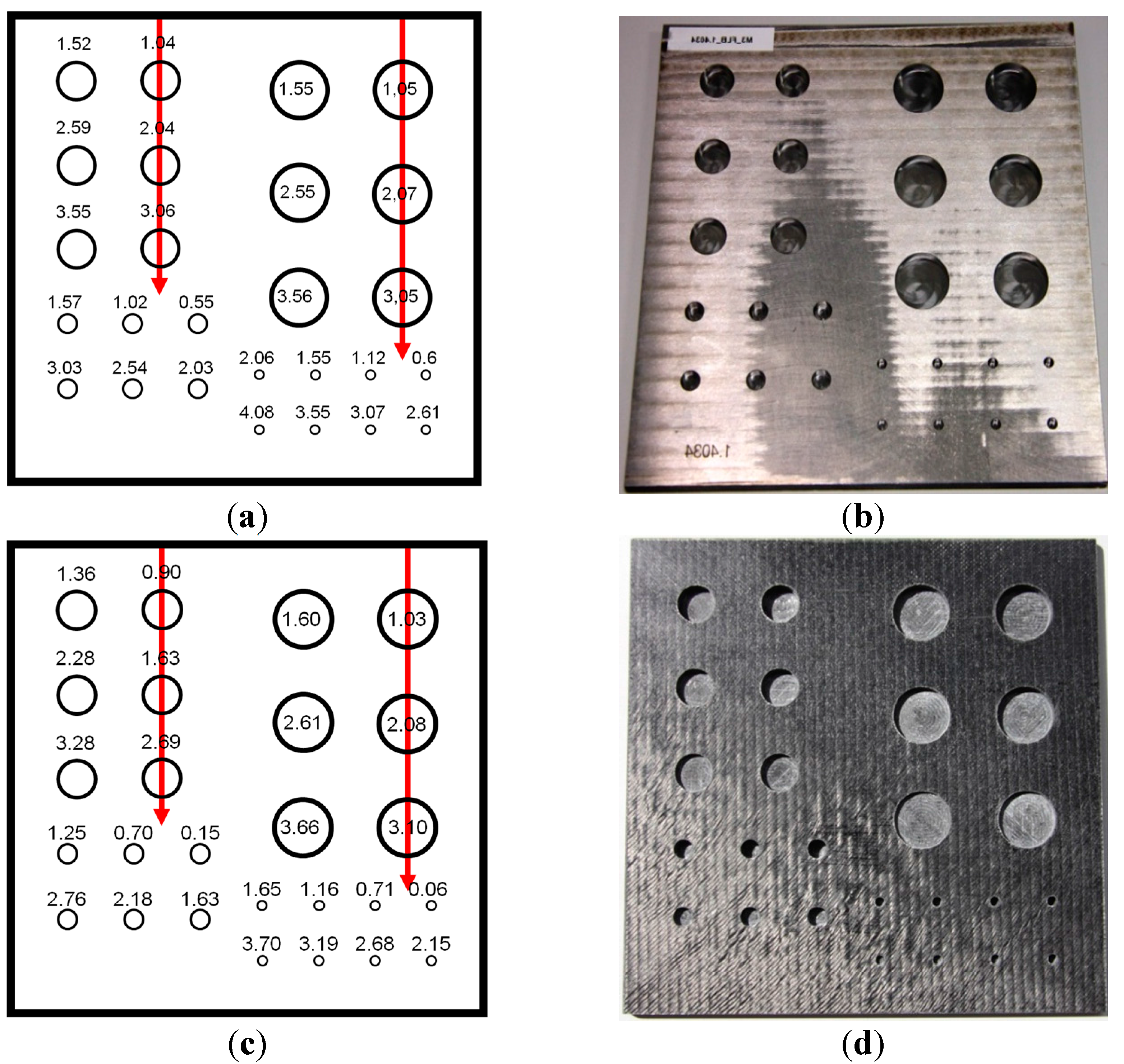
3.1.1. Test Specimens with Flat Bottom Holes

Test specimen no. 1.1 FBH consists of steel 1.4034, has a size of 200 mm × 200 mm × 6 mm and contains 26 FBHs with diameters of 24 mm, 16 mm, 8 mm, and 4 mm. A sketch of the test specimen indicating the RWTs of each hole is shown in Figure 2a, a photograph is displayed in Figure 2b.

Figure 2. Test specimens with flat bottom holes (FBH). (a,b) Test specimen no. 1.1 consisting of steel 1.4034 with a size of 200 mm × 200 mm × 6 mm. The given values are in mm and quantify the remaining wall thicknesses (RWT) of the holes. (c,d) Test specimen no. 1.2 consisting of CFRP with a size of 200 mm × 200 mm × 6 mm. The numbers indicate the RWT of the respective holes in mm. The red lines indicate line scans (see Section 4.1.3).

Figure 2. Test specimens with flat bottom holes (FBH). (a,b) Test specimen no. 1.1 consisting of steel 1.4034 with a size of 200 mm × 200 mm × 6 mm. The given values are in mm and quantify the remaining wall thicknesses (RWT) of the holes. (c,d) Test specimen no. 1.2 consisting of CFRP with a size of 200 mm × 200 mm × 6 mm. The numbers indicate the RWT of the respective holes in mm. The red lines indicate line scans (see Section 4.1.3).

Test specimen no. 1.2 FBH is made of 36 layers of a carbon fiber roving (100 g/m², biaxial ±45°) with a quasiisotropic layer adjustment being symmetrical to the middle (9 × +45/−45/0/90 and 9 × 90/0/+45/−45) and an epoxy matrix. It was constructed in 2012. The molding was performed by the RTM light method. Similar to no. 1.1, also this test specimen has a size of 200 mm × 200 mm × 6 mm and contains 26 flat bottom holes with diameters of 24 mm, 16 mm, 8 mm, and 4 mm. A sketch of the test specimen including the RWT of the holes is displayed in Figure 2c, a photograph is shown in Figure 2d. It has to be noted that the holes with a diameter of 24 mm of both test specimens have similar RWT, while for the holes with smaller diameters the RWT deviate strongly, since it was difficult to mill these holes in CFRP.

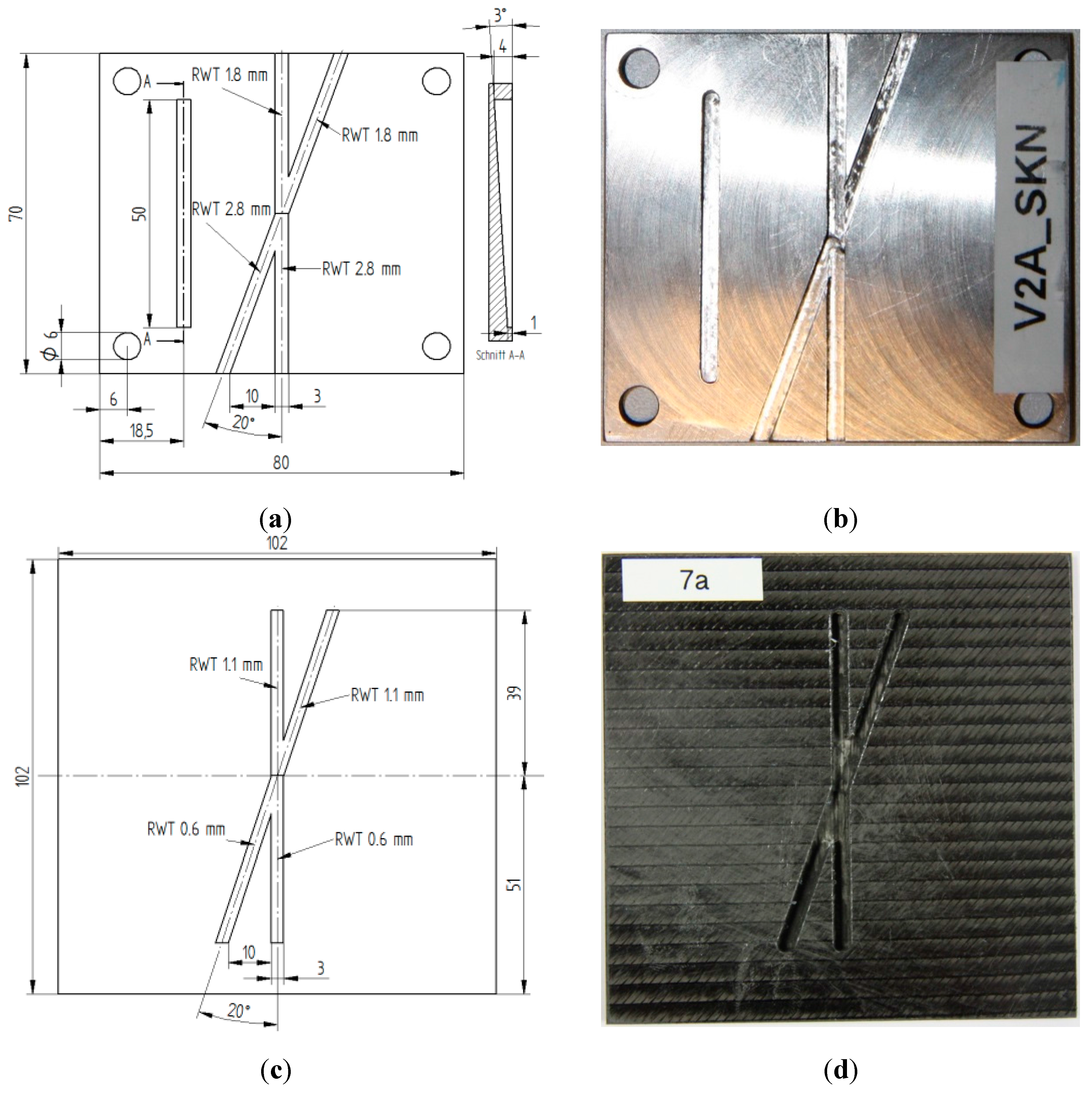
3.1.2. Test Specimens with Crossed Notches

Test specimen no. 2.1 is made of V2A steel (1.4301), has outer dimensions of 70 mm × 80 mm × 5 mm and contains two notches with a width of 3 mm which are crossing each other with an angle of 20°. On one side of the cross, the remaining wall thickness is 1.8 mm, on the other side 2.8 mm. Additionally, this test specimen contains a wedge with a width of 3 mm and remaining wall thicknesses starting at 3.7 mm and decreasing to 1.45 mm, which was not considered here. Figure 3a,b show a sketch and a photograph of this test specimen.

Test specimen no. 2.2 is made of 32 layers of a carbon fiber roving (100 g/m², biaxial ±45°) with a quasiisotropic layer adjustment being symmetrical to the middle (8 × +45/−45/0/90 and 8 × 90/0/+45/−45) and an epoxy matrix. It was constructed in 2014. Its outer dimensions are 102 mm × 102 mm × 6 mm and it contains two notches with a width varying between 3.2 and 3.8 mm, which are crossing each other with an angle of 20°. The remaining wall thicknesses of the notches are 0.6 and 1.1 mm, which are less than those of No. 2.1. This specimen does not contain a wedge as shown in the sketch and photograph in Figure 3c,d.

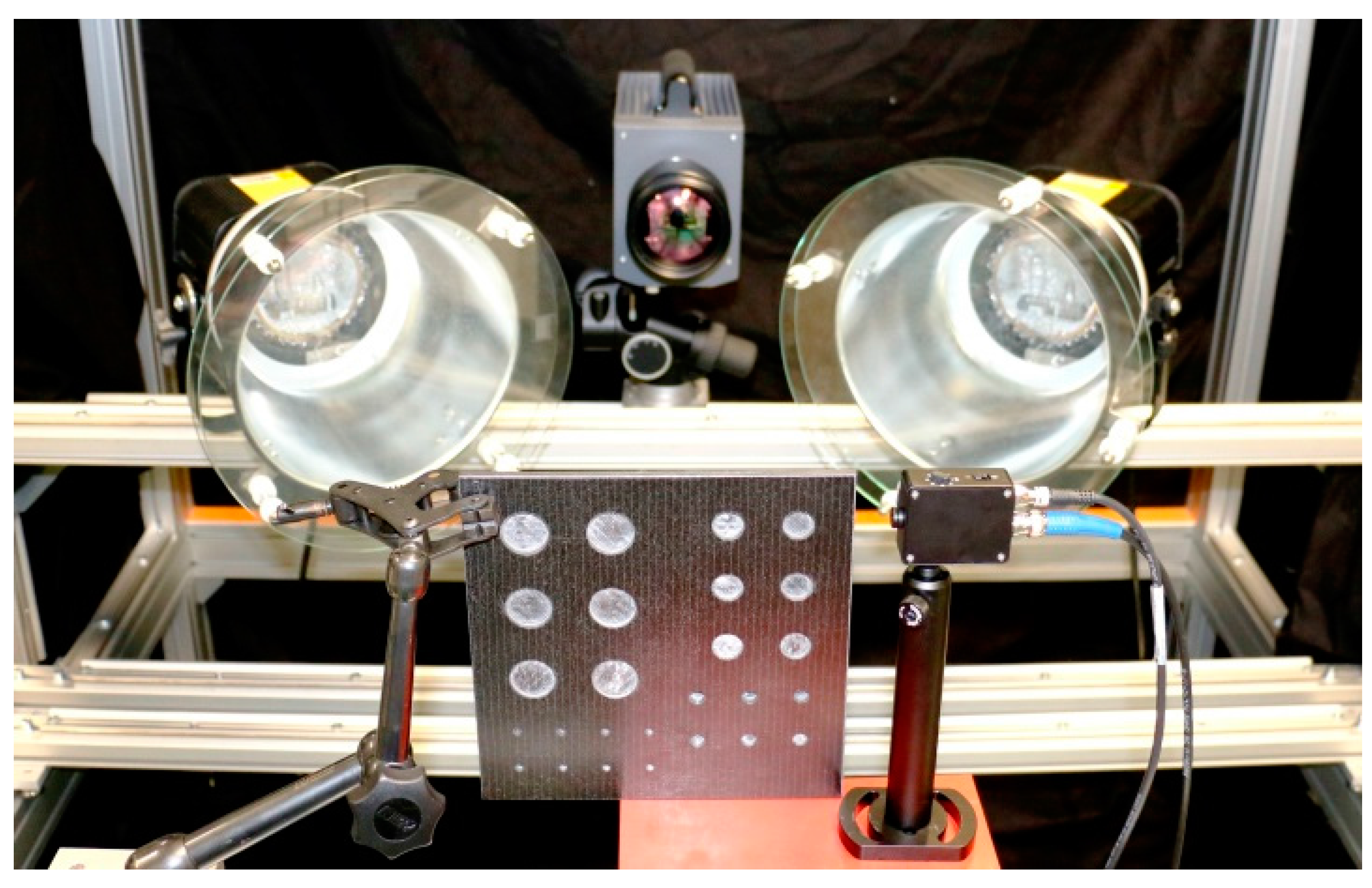
3.2. Experimental Set-up for Lockin Excitation

For lockin thermography, the object under investigation is heated periodically while the surface temperature is recorded simultaneously with an IR camera. To obtain amplitude and phase images in frequency domain, the recorded thermal response is correlated with the excitation signal. This can be done directly during the measuring (on-line lockin) or after the measurement (off-line lockin). In both cases the IR camera and the signal generator, which is controlling the heat sources, are synchronized. Advantages of on-line lockin are that amplitude and phase images are calculated during the measurements and the storage of long sequences, which might be a huge amount of data especially for large detectors, is not required. However, there are a number of disadvantages: Since the raw temperature data are not available, the data analysis cannot be adapted to the steady state situation, where phase contrast does not depend on time. Phase shifts between excitation and response signal cannot be corrected and different numbers of periods cannot be analyzed afterwards. Therefore, in the investigations presented herein, off-line lockin was utilized.

Figure 3. Test specimens with crossed notches at different depths. (a,b) Sketch and photo of crossed notches in V2A steel (test specimen no. 2.1) with remaining wall thicknesses (RWT) of 1.8 and 2.8 mm. (c,d) Sketch and photograph of crossed notches in quasiisotropic CFRP (test specimen no. 2.2) with RWT of 0.6 and 1.1 mm.

Figure 3. Test specimens with crossed notches at different depths. (a,b) Sketch and photo of crossed notches in V2A steel (test specimen no. 2.1) with remaining wall thicknesses (RWT) of 1.8 and 2.8 mm. (c,d) Sketch and photograph of crossed notches in quasiisotropic CFRP (test specimen no. 2.2) with RWT of 0.6 and 1.1 mm.

Figure 4 shows the experimental set-up. Two halogen lamps were used for periodic heating, each with a power consumption of 2250 W. These lamps were controlled by a frequency generator providing a sinusoidal voltage. The frequency generator was triggered by the IR camera to synchronize the data recording. To reduce disturbing IR radiation from the hot lamps, floatglass sheets were mounted in front of them. These soda lime silicate glass sheets have a low transmissivity for wavelengths above 2.5 µm, blocking the thermal radiation from the hot lamps effectively. The resulting increase in temperature of the floatglass sheets causes additional radiation as well, but significantly less than the direct radiation from the lamps. The distance of the lamps to the samples was about 500 mm. The lamps were positioned at the left and right side of the test specimen with an angle of about 30° to normal incidence. This was a compromise for achieving a high energy input and a homogeneous thermal distribution. Data recording was performed with a long wavelength IR camera. The used IR camera with a mercury cadmium telluride detector array is sensitive in the spectral range between 8 and 9.4 µm, thus the influence of direct light radiation from the halogen lamps should be effectively suppressed. The detector array has 640 × 512 pixels and a pixel pitch of 16 µm. A lens with a field of view of 23.1° × 18.6° was used. Since the camera was positioned at a distance of 650 mm to the samples, an area of 260 mm × 210 mm was recorded with a spatial resolution of about 0.41 mm/pixel (full frame). The noise equivalent temperature difference of this configuration was <60 mK measured at 30 °C with the selected integration time of 140 µs. At this integration time, a calibrated measurement range of 0 to 60 °C with a digitization depth of less than 14 bit and a sensitivity of 123 digits/K at 30 °C was selected.

Figure 4. Photograph of the experimental set-up for the lockin measurement showing the test specimen no. 1.1 in the front, the two halogen lamps with the glass filters and the IR camera in the back.

Figure 4. Photograph of the experimental set-up for the lockin measurement showing the test specimen no. 1.1 in the front, the two halogen lamps with the glass filters and the IR camera in the back.

The excitation frequencies were selected according to Figure 1. As the thickness of the samples was about 6 mm, lowest frequencies of 0.1 Hz and 0.01 Hz were selected for steel and CFRP, respectively, to enable phase contrast over the whole sample thickness. Afterwards, higher frequencies were also chosen for the detection of shallower defects. Concerning the number of the recorded periods, depending on the frequency, 3 to 10 periods are required to obtain a steady-state condition, i.e., a phase shift being constant in time. For data analysis, a minimum of one period has to be recorded. As the SNR is increasing with the number of recorded periods, more periods were chosen. An integer number of periods was always used. Table 2 gives an overview about the excitation frequencies, the recorded number of periods, the number of periods used for calculation of amplitude and phase images, the phase lag of the analyzed signal and the sampling rates applied for each material. These datasets were analyzed by FFT (Fast Fourier Transformation) using the given function in MATLAB2012a. The amplitude and phase images at these excitation frequencies are displayed with optimized contrast (see Figure 5).

Figure 5. Amplitude and phase images of the two test specimens with flat bottom holes recorded at different frequencies. The numbers above the respective images indicate the corresponding frequency and thermal diffusion length. The top row (a–d) shows the amplitude images of the steel sample No. 1.1 recorded at 1, 0.5, 0.2, and 0.1 Hz, respectively. The second row (e–h) shows the respective phase images. The third row (i–l) shows the sketch and the amplitude images of the CFRP sample No. 1.2 recorded at 0.1, 0.05, 0.02, and 0.01 Hz. The bottom row (m–p) shows the respective phase images.

Figure 5. Amplitude and phase images of the two test specimens with flat bottom holes recorded at different frequencies. The numbers above the respective images indicate the corresponding frequency and thermal diffusion length. The top row (a–d) shows the amplitude images of the steel sample No. 1.1 recorded at 1, 0.5, 0.2, and 0.1 Hz, respectively. The second row (e–h) shows the respective phase images. The third row (i–l) shows the sketch and the amplitude images of the CFRP sample No. 1.2 recorded at 0.1, 0.05, 0.02, and 0.01 Hz. The bottom row (m–p) shows the respective phase images.

Table 2. Parameters of lockin measurements and data analysis.

	Steel No. 1.1, 2.1	CFRP No. 1.2, 2.2
Lockin frequencies in Hz	0.1, 0.2, 0.5, 1	0.01, 0.02, 0.05, 0.1
Recorded periods	100	30 to 40
Periods used for calculation	last 80	last 20
Phase lag of first period for calculation	0° of thermal signal	0° of thermal signal
sampling rate (frame rate)	20 frames per period	20 frames per period

Table 2. Parameters of lockin measurements and data analysis.

	Steel No. 1.1, 2.1	CFRP No. 1.2, 2.2
Lockin frequencies in Hz	0.1, 0.2, 0.5, 1	0.01, 0.02, 0.05, 0.1
Recorded periods	100	30 to 40
Periods used for calculation	last 80	last 20
Phase lag of first period for calculation	0° of thermal signal	0° of thermal signal
sampling rate (frame rate)	20 frames per period	20 frames per period

4. Results

4.1. Test Specimens with Flat Bottom Holes

4.1.1. Comparison of Amplitude and Phase Images

The amplitude images of test specimen No. 1.1 (steel) recorded at 1, 0.5, 0.2 and 0.1 Hz and those of test specimen No. 1.2 (CFRP) recorded at 0.1, 0.05, 0.02, and 0.01 Hz are shown in the first and third row of Figure 5, respectively. These selected frequencies have comparable thermal diffusion length in both materials, which are also indicated in the figure. For both test specimens, it can be observed that with decreasing frequency (and thus increasing information depth), more FBHs are visible. Comparing these amplitude images, the following observations can be summarized:

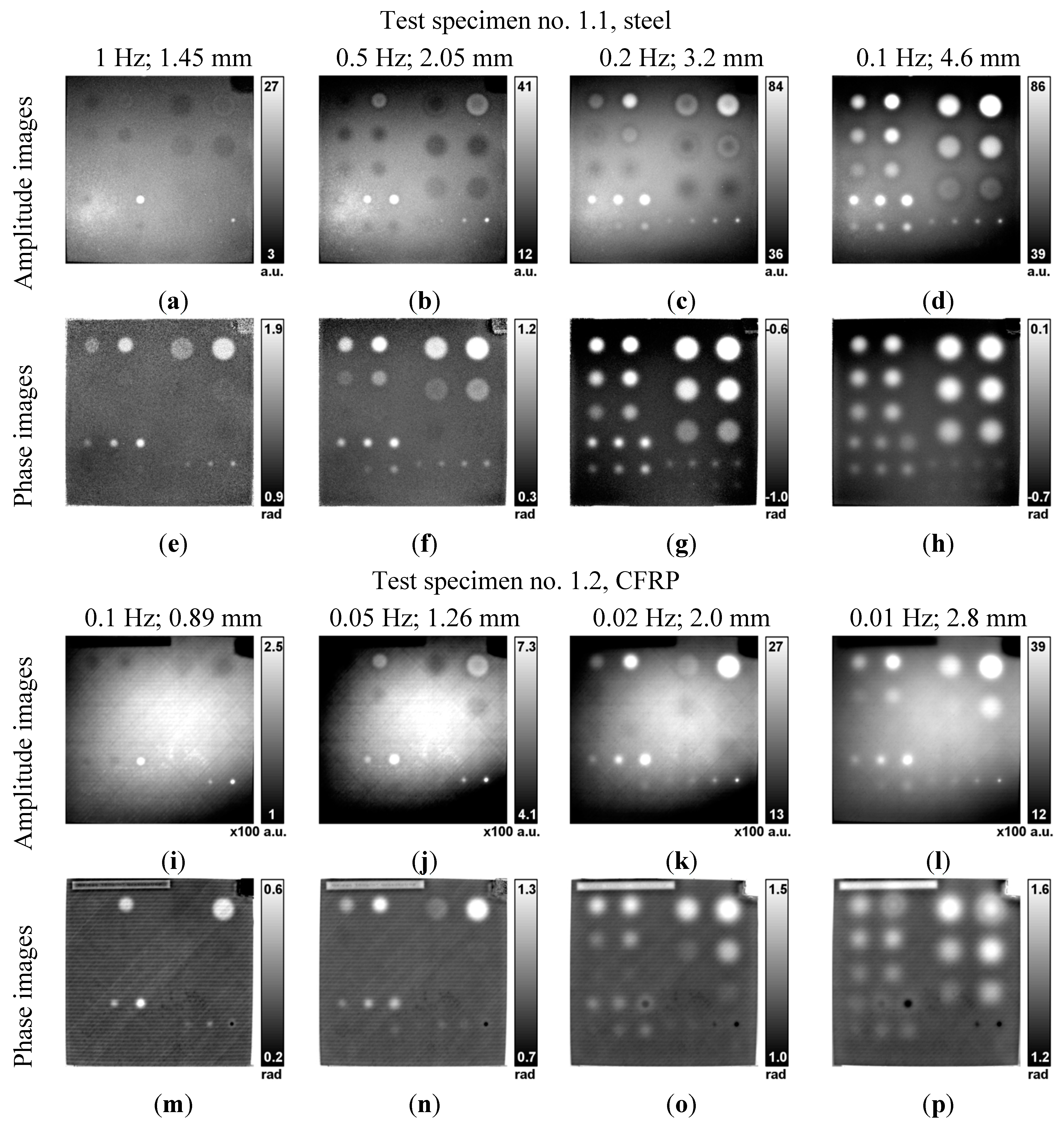
• In all amplitude images, an inhomogeneous background due to inhomogeneous heating can be observed.
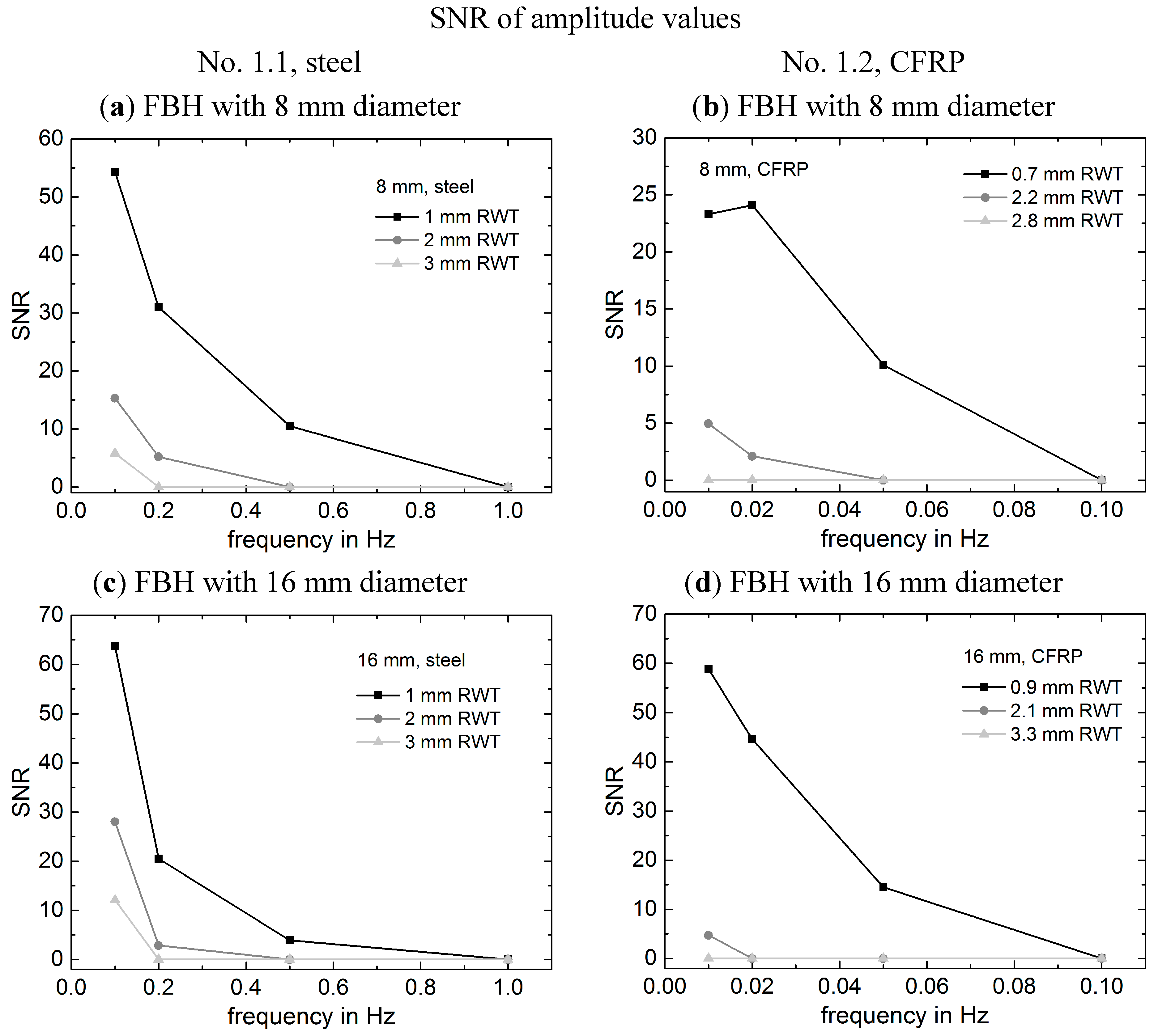
• For higher frequencies, the deeper holes appear with smaller (darker) amplitude values than the background. With decreasing frequency, the contrast switches and the holes appear with larger (brighter) values than the background. This can be explained by the minima in the amplitude values shown in Figure 1a,c.
• Comparing images of CFRP and steel, especially the smaller holes appear more blurred in the amplitude images of CFRP.
• In steel, all larger holes with diameters of 24, 16, and 8 mm are detected. For the holes with a diameter of 4 mm, only the upper row is detected, thus up to a RWT of 2.1 mm.
• In CFRP, less holes are detected: Only five of the 24 mm (up to a RWT of 3.1 mm), four of the 16 mm (up to a RWT of 2.3 mm), five of the 8 mm (up to a RWT of 2.2 mm) and again only the upper row of the 4 mm holes (up to a RWT of 1.65 mm) are detected.

The phase images of test specimen No. 1.1 (steel) and test specimen No. 1.2 (CFRP) are shown in the second and forth row in Figure 5. For both test specimens more FBHs become visible with decreasing frequencies and thus increasing thermal diffusion length. Comparing these phase images, the following observations can be summarized:

• In all phase images, the background appears homogenous.
• While the FBHs appear relatively sharp in the steel specimen, they are more blurred in the CFRP specimen.
• In the steel specimen, almost all FBHs can be detected; only the 4 mm hole with the thickest RWT cannot be seen in the phase image at 0.2 Hz.
• In the CFRP specimen, only four of the 4 mm holes are detected.
• In the CFRP specimen, two of the 8 mm holes (RWT of 0.15 and 0.7 mm) and two of the 4 mm holes (RWT of 0.06 and 0.71 mm) show a phase contrast inversion when going to lower frequencies, crossing the blind frequency.

By comparing the amplitude and phase images of each material, the following observations are made:

• As expected, the phase images show a homogeneous background while the amplitude images show an inhomogeneous background, caused by the inhomogeneous heating and cooling at the edges and corners.
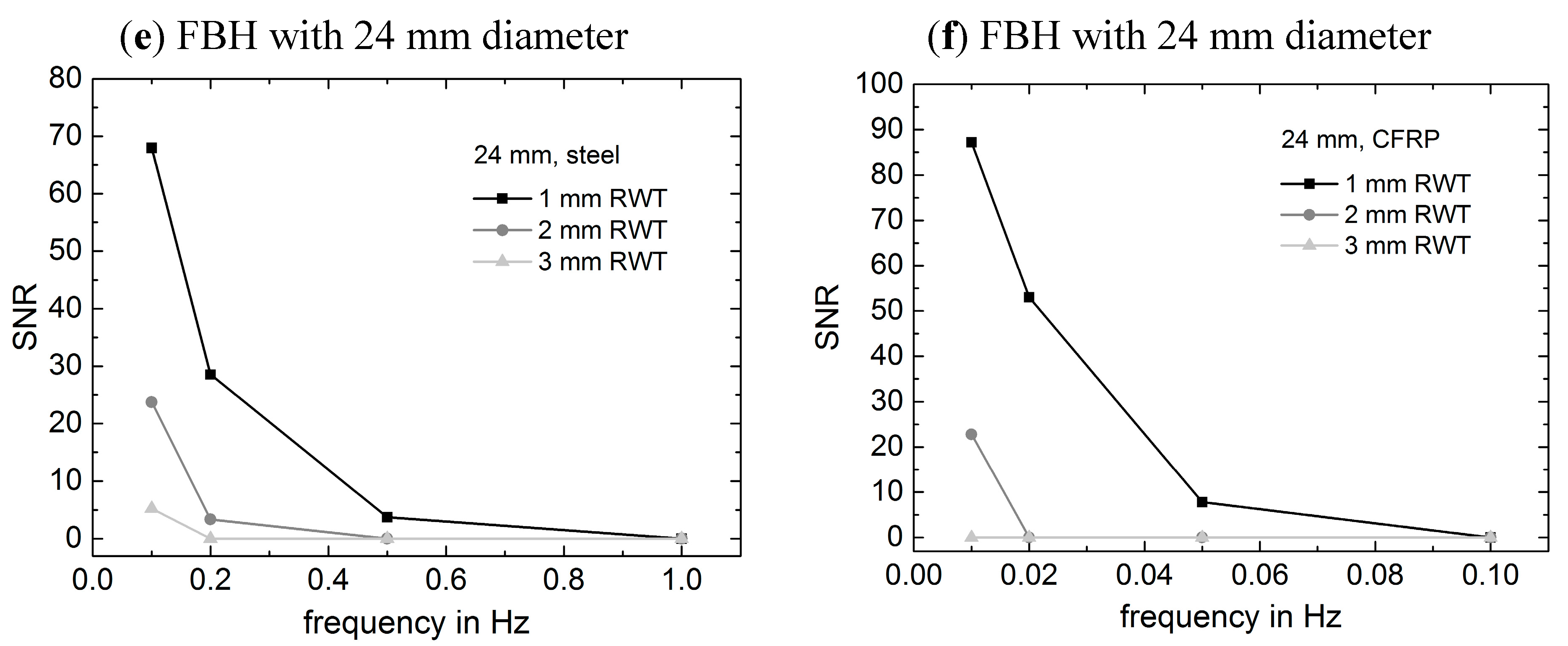
• In the phase images, deeper holes are detected than in the amplitude images.
• For the same frequency and the same hole in CFRP, the signatures appear in most cases more blurred in the phase images than in the amplitude images.

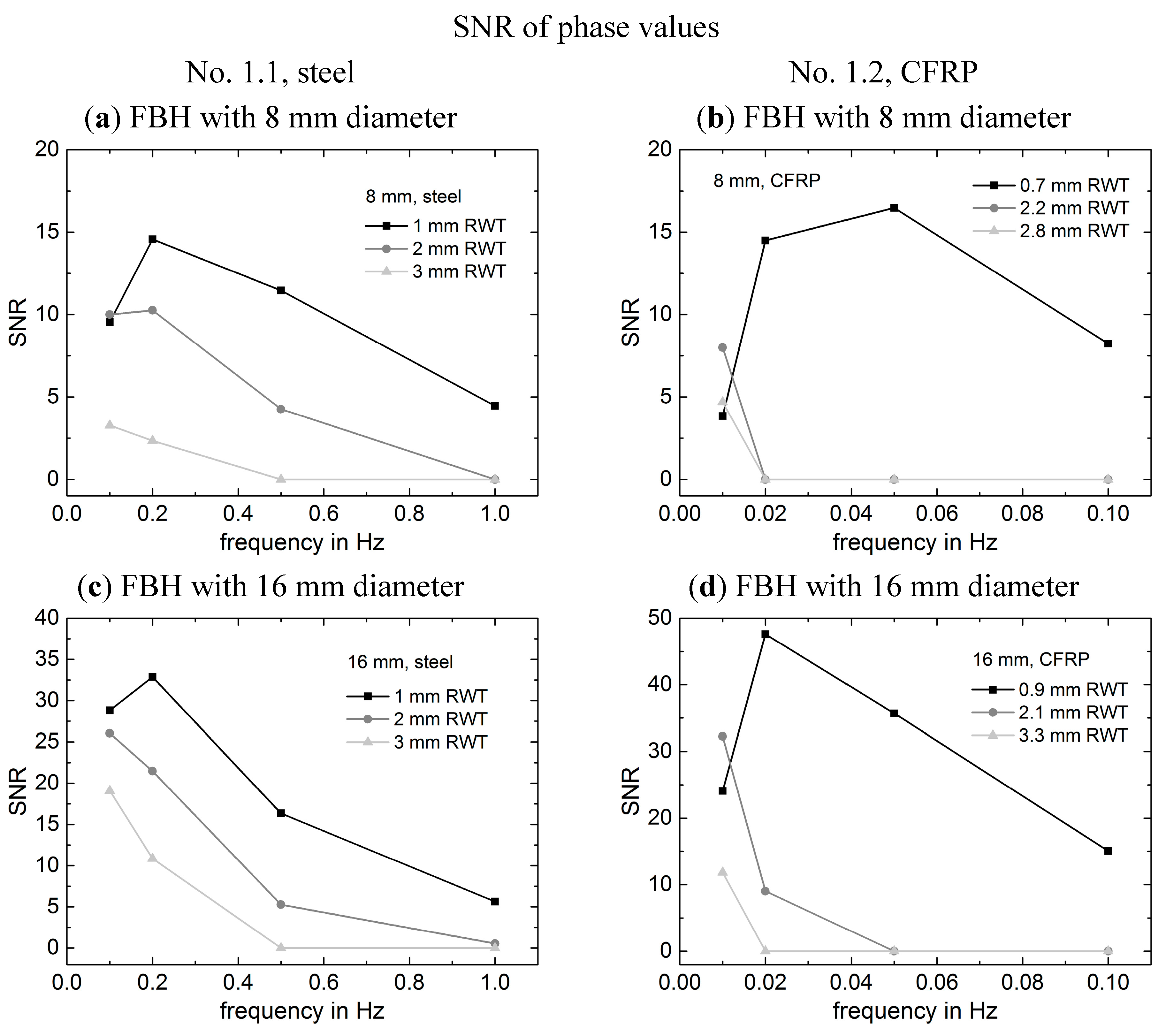
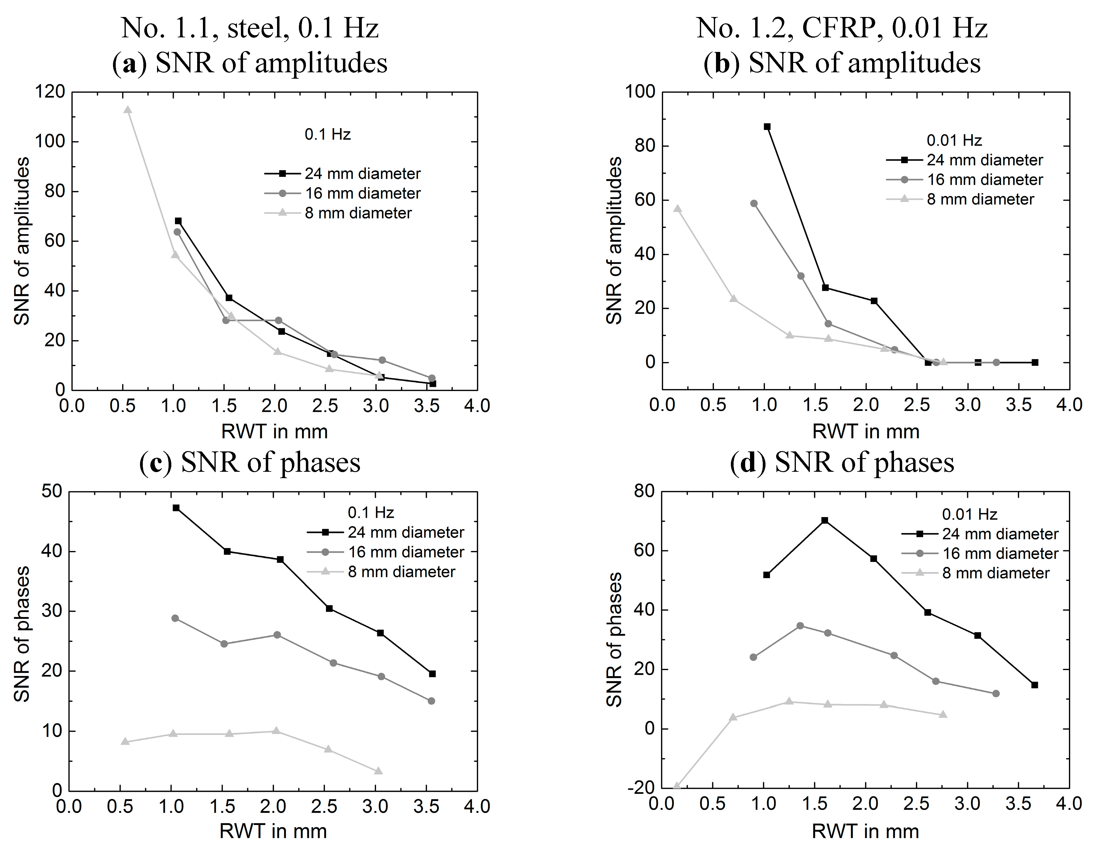
4.1.2. Analysis of Signal-to-Noise Ratio

The signal-to-noise ratio (SNR) of the amplitude and phase differences ΔA and Δφ of the FBHs was determined as follows:

$$SNR=\frac{\Delta A}{{\mathsf{\sigma }}_A}, SNR=\frac{\Delta \mathsf{\varphi }}{{\mathsf{\sigma }}_{\mathsf{\varphi }}}$$

(5)

The amplitude and phase differences, ΔA and Δφ, respectively, were determined from the difference of the maximum of the signal of each hole and the background close to the hole in respective line scans. For the amplitude values of the holes, only the values being higher (brighter) than the background were considered.

The noise σ was determined from the standard deviation of the amplitude and phase values in undisturbed areas of the specimen, respectively:

$${\mathsf{\sigma }}_A=\sqrt{\frac{1}{n-1}{\displaystyle \sum _{i=1}^n{(A_i-\overline{A})}^2}}, {\mathsf{\sigma }}_{\mathsf{\varphi }}=\sqrt{\frac{1}{n-1}{\displaystyle \sum _{i=1}^n{({\mathsf{\varphi }}_i-\overline{\mathsf{\varphi }})}^2}}$$

(6)

where n is the number of pixels of the selected areas, A_i and φ_i the amplitude and phase value of each pixel of the selected areas and $\overline{A}$ and $\overline{\mathsf{\varphi }}$ the mean value of these amplitude and phase values, respectively. Here, four areas with a size of 20 × 20 pixels were selected in each amplitude and phase image for the determination of the average noise value.

The SNRs of the amplitude and phase values are shown in the diagrams in Figure 6 and Figure 7, respectively. In each diagram, the SNRs from the FBHs with one diameter and three different remaining wall thicknesses are depicted as a function of excitation frequency. Since less periods have been recorded for the CFRP samples than for the steel samples, a comparison has to be interpreted carefully. Additionally, the SNR values of the amplitude and phase values of steel and CFRP are plotted as a function of the RWT in Figure 8 for the lowest frequency of each material (0.1 Hz for steel and 0.01 Hz for CFRP).

The following observations can be summarized for the amplitude images:

• In all cases, the SNR is higher for the FBHs with less RWT (see Figure 6). With increasing RWT, the SNR decreases exponentially (see Figure 8).
• For CFRP, the SNR increases with increasing diameter for the excitation frequencies of 0.01 and 0.02 Hz (see Figure 6 and Figure 8). For steel, no clear influence of the hole diameter can be observed (see Figure 8).
• With the exception of the shallow 8 mm hole in CFRP, the SNR is always decreasing with increasing frequency (see Figure 6).
• In most cases, the SNR values of steel are higher than those of CFRP. Only for the shallow 16 mm and 24 mm holes (1 mm RWT), the SNR values of CFRP are higher than those of steel (Figure 6 and Figure 8). But, as mentioned above, a less number of periods was recorded for CFRP.
• In steel, the FBHs are detected up to a RWT of 3.5 mm. In CFRP, the FBH are only detected up to a RWT of 2.5 mm (see Figure 8).

Figure 6. Signal-to-Noise Ratio (SNR) of measured amplitude differences at flat bottom holes (FBH) with remaining wall thicknesses of 1, 2, and 3 mm as a function of frequency. (a,b) SNR of the FBHs of test specimen No. 1.1 (steel) and of test specimen No. 1.2 (CFRP) with a diameter of 8 mm. (c,d) SNR of the FBHs of both test specimens with a diameter of 16 mm. (e,f) SNR of the FBHs of both test specimens with a diameter of 24 mm.

Figure 6. Signal-to-Noise Ratio (SNR) of measured amplitude differences at flat bottom holes (FBH) with remaining wall thicknesses of 1, 2, and 3 mm as a function of frequency. (a,b) SNR of the FBHs of test specimen No. 1.1 (steel) and of test specimen No. 1.2 (CFRP) with a diameter of 8 mm. (c,d) SNR of the FBHs of both test specimens with a diameter of 16 mm. (e,f) SNR of the FBHs of both test specimens with a diameter of 24 mm.

Figure 7. Signal-to-Noise Ratio (SNR) of measured phase differences at flat bottom holes (FBH) with remaining wall thicknesses of 1, 2, and 3 mm as a function of frequency. (a,b) SNR of the FBHs of test specimen No. 1.1 (steel) and of test specimen No. 1.2 (CFRP) with a diameter of 8 mm. (c,d) SNR of the FBHs of both test specimens with a diameter of 16 mm. (e,f) SNR of the FBHs of both test specimens with a diameter of 24 mm.

Figure 7. Signal-to-Noise Ratio (SNR) of measured phase differences at flat bottom holes (FBH) with remaining wall thicknesses of 1, 2, and 3 mm as a function of frequency. (a,b) SNR of the FBHs of test specimen No. 1.1 (steel) and of test specimen No. 1.2 (CFRP) with a diameter of 8 mm. (c,d) SNR of the FBHs of both test specimens with a diameter of 16 mm. (e,f) SNR of the FBHs of both test specimens with a diameter of 24 mm.

Figure 8. Measured signal-to-noise ratio (SNR) values as a function of the remaining wall thickness (RWT). (a) SNR of amplitude values of test specimen No. 1.1 (steel) recorded at 0.1 Hz; (b) SNR of amplitude values of test specimen No. 1.2 (CFRP) recorded at 0.01 Hz; (c) SNR of phase values of test specimen No. 1.1 (steel) recorded at 0.1 Hz; and (d) SNR of phase values of test specimen no. 1.2 (CFRP) recorded at 0.01 Hz.

Figure 8. Measured signal-to-noise ratio (SNR) values as a function of the remaining wall thickness (RWT). (a) SNR of amplitude values of test specimen No. 1.1 (steel) recorded at 0.1 Hz; (b) SNR of amplitude values of test specimen No. 1.2 (CFRP) recorded at 0.01 Hz; (c) SNR of phase values of test specimen No. 1.1 (steel) recorded at 0.1 Hz; and (d) SNR of phase values of test specimen no. 1.2 (CFRP) recorded at 0.01 Hz.

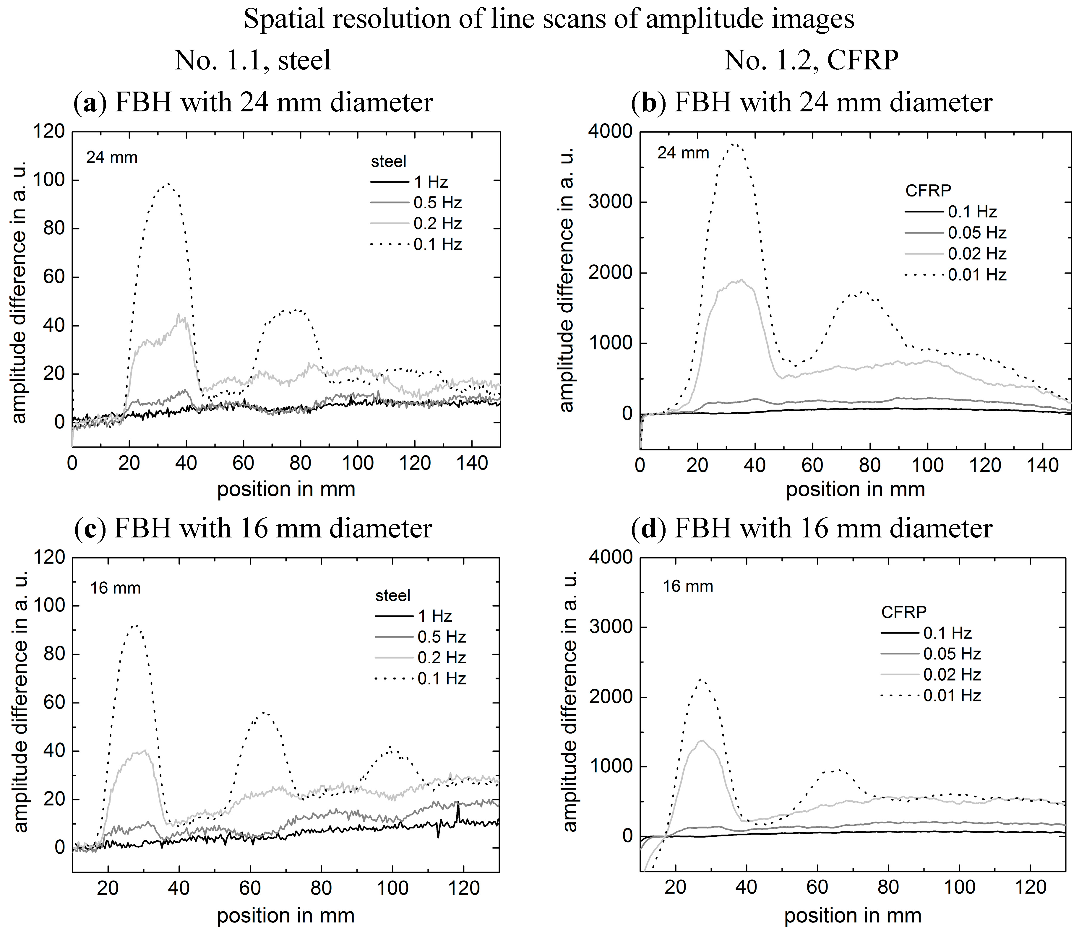
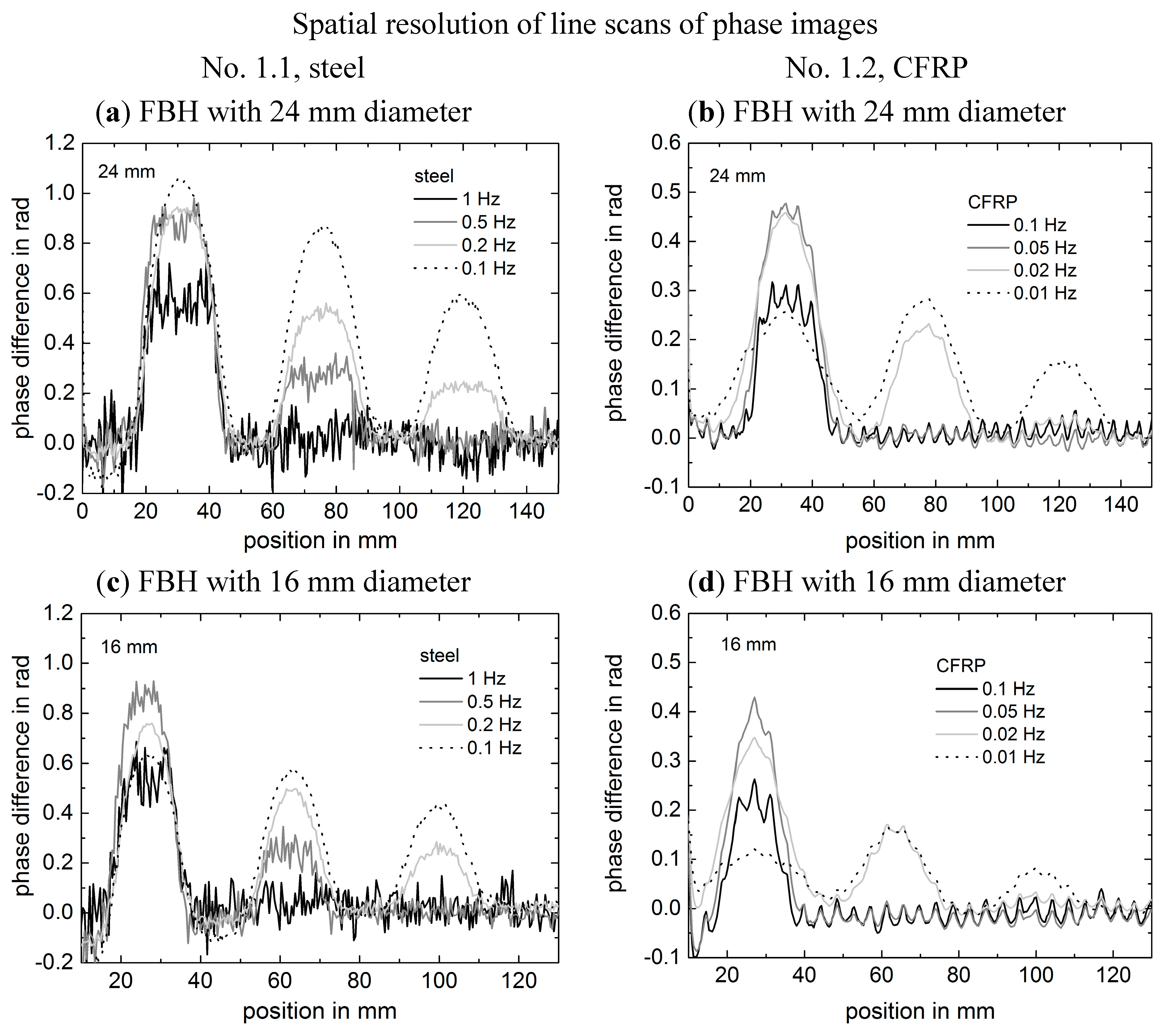
4.1.3. Analysis of Spatial Resolution

In the amplitude and phase images of Figure 5, it was already observed that the signatures of the FBHs in CFRP are appearing much more blurred than in steel, especially at low frequencies. A comparison of the amplitude and phase images shows that, in some cases, the phase signatures are appearing slightly more blurred than the amplitude signatures for the same FBH. For a more objective comparison, line scans recorded across three FBHs with a diameter of 24 mm and across three FBHs with a diameter of 16 mm were analyzed, as indicated by red lines in Figure 2a,c. The line scans are shown in Figure 9 and Figure 10 for four different frequencies for each test specimen and have been averaged along three adjacent lines taken from the respective images. Here, the following points can be summarized concerning the spatial resolution, which is here compared by the width (e.g., full width at half maximum, FWHM) of the signatures of the holes:

• Test specimen no. 1.1 (steel):

  ○

  Amplitude lines:

  ▪

  Due to the exponential decay of the amplitude differences with increasing RWT, only the shallowest hole is analyzed. The FWHM of the hole profiles show nearly no broadening with decreasing frequency for the 24 mm hole and a slight broadening for the 16 mm hole.

  ▪

  With decreasing frequency, a rounding of the more or less flat profile top of the shallowest hole for both diameters is observed.

  ○

  Phase lines:

  ▪

  Only a slight increase of the FWHM of the hole profiles occurs with decreasing frequency and with increasing RWT. This effect is slightly larger for the holes with a diameter of 16 mm.

  ▪

  Down to a frequency of 0.2 Hz, a plateau along the profile top above the FBHs is recognizable. These plateaus are most pronounced when the thermal diffusion length is smaller or equal to the RWT of the FBH.

  ○

  Comparison of amplitude and phase lines:

  ▪

  There is a clear difference in the background signal of the lines, which is larger and inhomogeneous in the amplitude line and is caused by the inhomogeneous heating.

  ▪

  For the detectable holes, there is no significant difference in the width of the profiles for the amplitudes and phases.

• Test specimen no. 1.2 (CFRP):

  ○

  Amplitude lines:

  ▪

  As for the amplitude lines of the steel sample, only the shallowest holes are analyzed. For both diameters, a slight increase of the peak width is observed with decreasing frequency. The width is also slightly larger than for holes with the same diameters in the steel sample.

  ○

  Phase lines:

  ▪

  First of all, for the higher frequencies (0.1 and 0.05 Hz), the structure of the fiber bundles is resolved.

  ▪

  Compared to the steel specimen, the FWHM of the FBHs is increased, which again more is pronounced for the FBHs with a diameter of 16 mm.

  ▪

  Only for the highest frequency of 0.1 Hz, a slight plateau can be observed in the profile of the shallowest FBH with a diameter of 24 mm.

  ○

  Comparison of amplitude and phase lines:

  ▪

  Only the amplitude lines show an inhomogeneous background.

  ▪

  The fiber bundles are only resolved in the phase images for the two higher excitation frequencies.

  ▪

  For the two lower frequencies, the phase profiles are significantly broader than the amplitude profiles.

Figure 9. Line scans of amplitude images above the flat bottom holes (FBH) along the red lines shown in Figure 2 recorded at different frequencies. (a,b) Line scans above FBHs with 24 mm diameter of test specimen No. 1.1 (steel) and test specimen No. 1.2 (CFRP) with remaining wall thickness of 1 mm, 2 mm and 3 mm (from left to right). (c,d) Line scans above FBHs with 16 mm diameter of both test specimens with remaining wall thickness of 1 mm, 2 mm and 3 mm (from left to right).

Figure 9. Line scans of amplitude images above the flat bottom holes (FBH) along the red lines shown in Figure 2 recorded at different frequencies. (a,b) Line scans above FBHs with 24 mm diameter of test specimen No. 1.1 (steel) and test specimen No. 1.2 (CFRP) with remaining wall thickness of 1 mm, 2 mm and 3 mm (from left to right). (c,d) Line scans above FBHs with 16 mm diameter of both test specimens with remaining wall thickness of 1 mm, 2 mm and 3 mm (from left to right).

Figure 10. Line scans of phase images above the flat bottom holes (FBH) along the red lines shown in Figure 2 recorded at different frequencies. (a,b) Line scans above FBHs with 24 mm diameter of test specimen No. 1.1 (steel) and of test specimen No. 1.2 (CFRP). (c,d) Line scans above FBHs with 16 mm diameter of both test specimens.

Figure 10. Line scans of phase images above the flat bottom holes (FBH) along the red lines shown in Figure 2 recorded at different frequencies. (a,b) Line scans above FBHs with 24 mm diameter of test specimen No. 1.1 (steel) and of test specimen No. 1.2 (CFRP). (c,d) Line scans above FBHs with 16 mm diameter of both test specimens.

4.2. Test Specimens with Crossed Notches

For a comparison between data of test specimens No. 2.1 and 2.2, it has to be considered that the RWT above the notches of test specimen No. 2.1 and No. 2.2 are different: the RWT of the notches of No. 2.1 are 1.8 and 2.8 mm, while the RWT of the notches of No. 2.2 are 0.6 and 1.1 mm.

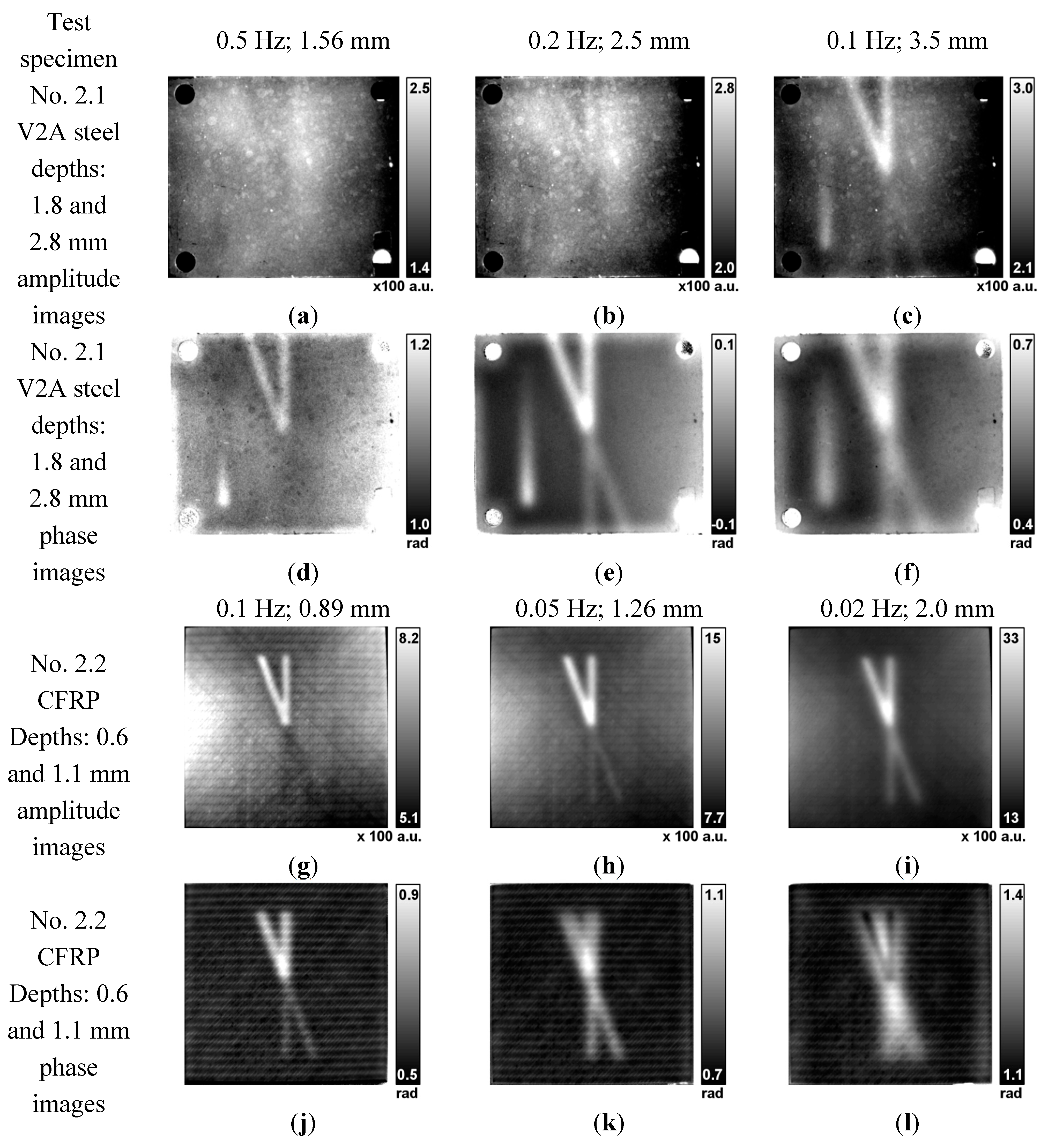
4.2.1. Comparison of Amplitude and Phase Images of the Steel Sample no. 2.1

Amplitude and phase images recorded at 0.5, 0.2, and 0.1 Hz for test specimen No. 2.1 (steel) are shown in the first and second row of Figure 11.

Figure 11. Amplitude and phase images of the two test specimen with crossed notches recorded at different frequencies. The numbers above the respective images indicate the corresponding frequency and thermal diffusion length (Equation (2)). (a–c) Test specimen No. 2.1, V2A steel, amplitude images at frequencies of 0.5, 0.2, and 0.1 Hz and (d–f) respective phase images. (g–i) Test specimen No. 2.2, quasiisotropic CFRP, amplitude images at frequencies of 0.1, 0.05, and 0.02 Hz and (j–l) respective phase images.

Figure 11. Amplitude and phase images of the two test specimen with crossed notches recorded at different frequencies. The numbers above the respective images indicate the corresponding frequency and thermal diffusion length (Equation (2)). (a–c) Test specimen No. 2.1, V2A steel, amplitude images at frequencies of 0.5, 0.2, and 0.1 Hz and (d–f) respective phase images. (g–i) Test specimen No. 2.2, quasiisotropic CFRP, amplitude images at frequencies of 0.1, 0.05, and 0.02 Hz and (j–l) respective phase images.

The following observations can be summarized:

• Amplitude images:

  ○

  Only at the lowest excitation frequency of 0.1 Hz with a diffusion length of 3.5 mm, the shallow notch (RWT 1.8 mm) is detected clearly. At higher frequencies, only a very weak structure with amplitudes lower (0.5 Hz) and higher (0.2 Hz) than the background is visible. The deep notches (RWT 2.8 mm) are only detected with a very weak amplitude at the lowest frequency of 0.1 Hz.

• Phase images:

  ○

  At high frequencies, first the shallow notches are visible, while the deeper notches become clearer at lower frequencies. This is caused by the thermal diffusion lengths, which increase with decreasing frequency.

• Comparison of amplitude and phase images:

  ○

  In the amplitude images, the notches become apparent at frequencies belonging to a diffusion length that is considerably larger than the RWT. In the phase images, the notches appear already at a diffusion length smaller than the RWT.

  ○

  A comparison of the images at 0.1 Hz shows a higher lateral spatial resolution of the crossed notches in the amplitude image. A similar or even better resolution in the phase images is only obtained, if these have been recorded at higher frequencies (0.5 Hz).

4.2.2. Comparison of Amplitude and Phase Images of the CFRP Samples No. 2.2

The third and fourth row in Figure 11 show amplitude and phase images recorded at 0.1, 0.05, and 0.02 Hz for test specimen No. 2.2 (CFRP). The following observations can be summarized:

• Amplitude images:

  ○

  Already at the highest excitation frequency all notches are detected, albeit with different signs of the contrast: the shallow notches are appearing with a larger, the deeper notches with a slightly smaller amplitude than the background. With decreasing frequency, all notches appear with higher amplitude than the background.

  ○

  The structures only appear slightly blurred at lower frequencies and larger RWT.

  ○

  The diffusion lengths corresponding to the excitation frequencies at which the notches become visible more or less coincide with the RWT.

• Phase images:

  ○

  The deeper notches are already detected at a diffusion length that is smaller than the RWT.

  ○

  At the lowest frequency, the shallow notches show a phase contrast inversion.

  ○

  With decreasing frequency, a considerable blurring of the signature of the notches is observable.

• Comparison of amplitude and phase images:

  ○

  In the amplitude images, the notches become observable at frequencies that belong to diffusion length coinciding with the RWT. In the phase images, the notches already appear at diffusion lengths smaller than the RWT.

  ○

  The comparison of all images shows a higher lateral spatial resolution of the crossed notches in the amplitude images.

5. Discussion

5.1. Detectability of Defects

The investigations show that the detectability of defects (here: FBH and notches) in amplitude and phase images depends on RWT of FBH and notches and lateral size of the defects as well as on the thermal diffusivity of the surrounding material and its anisotropy. The detectability also depends on the applied excitation frequency. Although it was expected that the phase images will show an information depth which is about a factor of two larger than that of the amplitude images, this was not revealed by the experimental data. In steel, all FBH with a diameter of 24, 16 and 8 mm and RWT of up to 3.5 mm were detected in both the amplitude and phase images. In CFRP, the FBH with diameters of 24, 16 and 8 mm were detected up to a RWT of 2.5 mm in the amplitude images. In the phase images they were detected for a RWT of up to 3 mm for the 8 mm FBH, 3.3 mm for the 16 mm FBH, and 3.7 mm for the 24 mm holes.

In steel (test specimen no. 1.1), almost all FBHs with RWTs of up to 3.5 mm and diameters of 24, 16, 8, and 4 mm were detected in the phase images using an excitation frequency of 0.2 Hz, which corresponds to a thermal diffusion length of 3.2 mm (see Figure 5). Only two holes with a diameter of 4 mm and with RWT of 3.5 and 4 mm were not detected, thus the limit is at a RWT of 3 mm. This is mainly due to lateral thermal heat diffusion which reduces the phase contrast as well as the SNR, and which has a higher influence on small defects. It was not possible to detect these two holes by applying lower frequencies, e.g., 0.1 Hz. This is at least partially in contradiction to what was observed by Wallbrink et al. [15], who found that an excitation frequency of 0.02 Hz provides best thermal contrast for defects with a RWT of up to 9 mm in steel. At this frequency, the spatial resolution becomes worse and the defect depth cannot be calculated using simple analytical one-dimensional solutions. In Wallbrinks presentation, a phase image recorded at an excitation frequency of 0.1 Hz was shown, in which a similar number of defects can be detected as at 0.02 Hz. In the amplitude images of Figure 5, the holes with a diameter of 4 mm are only detected up to a RWT of 2.1 mm. Thus, the information depth in the phase images is higher, but not twice as high as for the amplitude images. Again, this is explained by lateral thermal diffusion effects due to the small size of the defects.

In quasiisotropic CFRP (test specimen no. 1.2), all FBHs with diameters of 24 and 16 mm with a RWT of up to 3.7 mm were detected in the phase images (see Figure 5). For the 8 mm diameter, only five FBHs were detected up to a RWT of 3 mm. Only four holes with a diameter of 4 mm are visible, which corresponds here to a detectability up to a RWT of only 1.6 mm. All holes except those with a diameter of 4 mm were detected in the phase image with the lowest excitation frequency of 0.01 Hz. Again, these limits of detectability are mainly due to lateral heat diffusion, which for CFRP is larger parallel to the surface than perpendicular to it. In the amplitude images, fewer holes were detected for the larger diameters. Only five of the 24 mm (up to a RWT of 3.1 mm) and four of the 16 mm (up to a RWT of 2.3 mm) are visible. For the smaller holes, the same holes were detected in the amplitude as in the phase images.

In comparison, slightly fewer defects were detected in CFRP than in steel.

Although the halogen lamps were positioned to achieve a high energy input and a homogeneous heating as well, the amplitude images show an inhomogeneous distribution of temperature with a maximum in the middle of the samples and smaller values at the edges and especially at the corners. Additional to an inhomogeneous heating, an enhanced cooling at the edges increases the temperature drop towards the edges, which could be avoided by using larger test specimens or thermal isolations of the edges. This inhomogeneity might also have reduced the detectability of the second row of FBH with a diameter of 4 mm, which was positioned close to the bottom right corner. To address this issue quantitatively, the raw thermogram sequences of the test specimens no. 1.1 (steel) and 1.2 (CFRP) were evaluated. In each sequence, a thermogram at the maximum heating of the last recorded period was selected. A thermogram recorded before heating was subtracted, thus the temperature increase was deduced. Mean values were calculated from small areas in the middle and the bottom right corner of the thermogram. For the steel sample and an excitation frequency of 0.1 Hz, a mean temperature increase of 12.2 K and 8.9 K was calculated in the middle and in the bottom right corner, respectively. Although this is clearly a difference, still a large amount of heat was introduced at the position of the 4 mm holes. For CFRP, in the sequence with an excitation frequency of 0.01 Hz, a mean temperature increase of 24.5 K was measured in the middle and of 11.1 K in the bottom right corner. Here, the temperature increase in the middle is more than twice as high as in the corner and cannot be neglected any more in the comparison of the detectability.

5.2. SNR of Defects

Figure 6 and Figure 7 show that the SNR increases with decreasing RWT. This effect is stronger for the amplitude signals than for the phase signals, since the amplitudes decrease exponentially with RWT. Regarding holes with a RWT >1 mm in both materials, the SNR of the holes is larger in the phase images than in the amplitude images for each frequency. This is in good agreement with the observation of Chatterjee et al. [3] for CFRP. For low frequencies, the shallowest holes with diameters down to 8 mm (only the SNR of the 24, 16 and 8 mm holes were analyzed) are detected best in the amplitude images, the other ones in the phase images. A clear influence of the diameter is only observed for the phase images: for a fixed RWT, the SNR increases with increasing diameter. For the amplitude images, no clear influence of the diameter was observed. This behavior can be explained by lateral thermal diffusion effects, which have a higher influence on phase images (due to a higher information depth) than on amplitude images.

For each material, the same number of periods was recorded for all frequencies and the number of recorded frames per period was kept constant, thus it is expected that the noise was similar in the phase and amplitude images. Therefore, at a first glance the SNRs should only depend on the amplitude and phase values as predicted in Figure 1. However, this relation was observed only for the larger and deeper defects in both materials. For the phase values of the shallower and smaller defects, a saturation or even a decrease of SNRs with decreasing frequency were observed. This effect is larger for the small diameters, thus it can be related to the lateral thermal diffusion. As mentioned above, the lateral thermal diffusion has a larger influence on the phase images.

Comparing the SNRs of both materials, the following tendency is noticed: for shallow and larger holes, the SNR of the signals in both amplitude and phase images is higher for CFRP, which can be explained by the slightly steeper curves of amplitude and phase in Figure 1. For deeper and smaller FBHs, the SNR in the CFRP images is lower than in the steel images, which can be explained by three effects:

• by the curve shapes in Figure 1 for the deeper and larger FBH,
• by the less number of periods recorded for the CFRP test specimens, and
• by the higher lateral diffusivity compared to the diffusivity in depth direction in CFRP.

In conclusion, to gain high defect detectability, an excitation frequency corresponding to a thermal diffusion length that is slightly larger than the expected depth of the defects should be selected. Only in this case, a maximum SNR expected. If the thermal diffusion length is considerably smaller than the defect depth, the defect might not be detectable. However, if the thermal diffusion length is too large, the influence of lateral heat diffusion reduces the SNR and, additionally, it reduces the spatial resolution as discussed in the following.

5.3. Spatial Resolution

For the investigation of the spatial resolution in steel and CFRP, line scans of amplitude and phase images above FBHs (as shown in Figure 9 and Figure 10) and above crossed notches (as shown in Figure 11) were compared, both for steel and CFRP.

The line scans of the FBHs show that with decreasing frequency and thus increasing thermal diffusion length, the flat profiles are blurred. The line scans of the phase images indicate a slight broadening of the profiles in steel, while a more distinct broadening of the profiles is observed for CFRP. In the amplitude lines, this effect is much smaller than in the phase lines.

In the amplitude and phase images of the crossed notches it is observed that the best spatial resolution is obtained in the amplitude images and at the highest excitation frequency, at which a significant amplitude or phase contrast of the structure is obtained. Concerning the influence of RWT, the shallower notches appear slightly sharper than the deeper ones. The signatures of the notches are broadening significantly with decreasing frequency, especially in CFRP phase images. All of these effects can be explained by the lateral thermal diffusivity:

• Since the thermal diffusion length µ is increasing with decreasing frequency, the lateral thermal diffusion length is increasing as well, leading to a lateral broadening of the signal.
• Due to the higher information depth in phase images than in amplitude images, the lateral information length is larger as well. Therefore, phase images have a smaller lateral resolution than amplitude images at a given excitation frequency.
• Since the thermal diffusivity in CFRP is larger laterally than in the depth direction, the lateral thermal diffusion length is also larger than the (perpendicular) diffusion length and the magnitude of these effects is enhanced.

6. Summary and Conclusions

In this study, systematic investigations using lockin thermography at materials with isotropic (steel) and anisotropic (CFRP) thermal material properties were performed. In order to address different aspects (the determination of detectability, SNR, and spatial resolutions of defects) test specimens with FBHs with varying RWT and diameters as well as specimens with crossed notches at different RWT were investigated. Except for the excitation frequency f, the measurement parameters were kept constant for both materials. To keep a comparable thermal diffusion length, the excitation frequency was varied between 0.1 to 1 Hz for steel and between 0.01 to 0.1 Hz for CFRP. The number of periods used for the calculation of the phase images was kept constant for each material (80 periods for steel and 20 periods for CFRP).

In steel, all of the FBHs with diameters of 24, 16, and 8 mm were detected. They have a maximum RWT of 3.5 mm. The FBHs with a diameter of 4 mm were detected up to a RWT of 3 mm. The best frequency for defect detection within the chosen experimental range was 0.1 Hz. In the case of quasiisotropic CFRP, all of the FBHs with diameters of 24, 16, and 8 mm were detected as well, and at a frequency of 0.01 Hz. They have a maximum RWT of 3.6 mm. Regarding defects with 4 mm diameter, only those with a maximum depth of 1.6 mm were detected.

As expected, for both materials and all defects the SNR was higher for the shallower defects and it was mostly increasing with decreasing frequency. Only for the shallower defects, the SNR in phase images had a maximum at a distinct excitation frequency. This effect was stronger for smaller diameters. For the shallower and larger defects, the SNR of the amplitude was higher than the SNR of the phase. A clear influence of the diameter was only observed for the phase images: for a fixed RWT, the SNR increases with increasing diameter. For the amplitude images, no clear influence of the diameter was observed.

For both materials, the spatial resolution was best for the highest frequency, at which the defect could be detected well, i.e., where a considerable signal difference and SNR was present. If the defect was detected in the amplitude as well as in the phase image, the spatial resolution was always better in the amplitude image, which could be seen best for the crossed notches. For similar defects, the spatial resolution was better in steel than in CFRP.

In conclusion, the lateral thermal diffusion influences the results of lockin thermography in the following way:

• In both amplitude and phase images, the signatures of defects become broader with decreasing frequency. This effect is much larger for the phase images. Therefore, the lateral spatial resolution is always better for the amplitude images and increases with the excitation frequency.
• This effect is stronger for materials with anisotropic thermal diffusivity, if the diffusivity is higher in the plane parallel to the surface than perpendicular to it, like in CFRP.
• The SNR in the phase images decreases with decreasing diameter of the defects for similar RWT and excitation frequency.
• The limit of RWT of the detected holes is less than twice as large for the phase images as for the amplitude images.

Further effects, which reduce the detectability as well as the SNR, are:

• The inhomogeneous temperature distribution due to inhomogeneous heating and faster cooling at the corners lead to a reduced detectability and SNR in the colder regions compared to the center region.
• Decreasing SNRs in the phase images for FBHs with larger diameter at lower excitation frequencies are related to the blind frequency.

References

1. Maierhofer, C.; Myrach, P.; Röllig, M.; Steinfurth, H. Validation of active thermography techniques for the characterization of CFRP structures. In Proceedings of the 11th European Conference on Non-Destructive Testing (ECNDT), Prague, Czech Republic, 6–10 October 2014.
2. Montanini, R. Quantitative determination of subsurface defects in a reference specimen made of Plexiglas by means of lock-in and pulse phase infrared thermography. Infrared Phys. Technol. 2010, 53, 363–371. [Google Scholar] [CrossRef]
3. Chatterjee, K.; Tuli, S.; Pickering, S.G.; Almond, D.P. Matched excitation energy comparison of the pulse and lock-in thermography NDE techniques. NDT E Int. 2011, 44, 655–667. [Google Scholar] [CrossRef] [Green Version]
4. Röllig, M.; Steinfurth, H.; Ziegler, M. Untersuchung von Hochleistungs-LEDs für den Einsatz in der zerstörungsfreien Prüfung mittels Thermografie. In Proceedings of the 2013 Thermografie-Kolloquium, Stuttgart, Germany, 26–27 September 2013.
5. Vavilov, V.P.; Almond, D.P.; Busse, G.; Grinzato, E.; Krapez, J.-C.; Maldague, X.; Marinetti, S.; Peng, W.; Shirayev, V.; Wu, D. Infrared thermographic detection and characterisation of impact damage in carbon fiber composites: Results of the round robin test. In Proceedings of the 1998 QIRT, Lodz, Poland, 7–10 September 1998.
6. Almond, D.P.; Ball, R.J.; Dillenz, A.; Busse, G.; Krapez, J.-C.; Galmiche, F.; Maldague, X. Round Robin comparison II of the capabilities of various thermographic techniques in the detection of defects in carbon fibre composites. In Proceedings of the 2000 QIRT, Reims, France, 18–21 July 2000.
7. Ibarra-Castanedo, C.; Piau, J.-M.; Guilbert, S.; Avdelidis, N.P.; Genest, M.; Bendada, A.; Maldague, X.P.V. Comparative study of active thermography techniques for the non-destructive evaluation of honeycomb structures. Res. Nondestr. Eval. 2009, 20, 1–31. [Google Scholar] [CrossRef]
8. Dillenz, A.; Wu, D.; Breitrück, K.; Busse, G. Lock-in thermography for depth resolved defect characterisation. In Proceedings of the 2000 WCNDT, Rome, Italy, 15–21 October 2000.
9. Giorleo, G.; Meola, C.; Squillace, A. Analysis of Defective Carbon-Epoxy by Means of Lock-in Thermography. Res. Nondestr. Eval. 2000, 12, 241–250. [Google Scholar] [CrossRef]
10. Zoecke, C.; Langmeier, A.; Arnold, W. Size retrieval of defects in composite material with lockin thermography. J. Phys. Conf. Ser. 2010, 214, 012093. [Google Scholar] [CrossRef]
11. Patel, P.M.; Almond, D.P. Thermal wave testing of plasma-sprayed coatings and a comparison of the effects of coating microstructure on the propagation of thermal and ultrasonic waves. J. Mater. Sci. 1985, 20, 955–966. [Google Scholar] [CrossRef]
12. Wu, D.; Busse, G. Lock-in thermography for non-destructive evaluation of materials. Rev. Gen. Therm. 1998, 37, 693–703. [Google Scholar] [CrossRef]
13. Spießberger, C.; Dillenz, A.; Zweschper, T. Active Thermography for quantitative NDT of CFRP components. In Proceedings of the 2nd International Symposium on 2010 NDT in Aerospace, Hamburg, Germany, 22–24 November 2010.
14. Meola, C.; Calomagno, G.M.; Giorleo, L. Geometrical Limitations to Detection of Defects in Composites by Means of Infrared Thermography. J. Nondestr. Eval. 2004, 23, 125–132. [Google Scholar] [CrossRef]
15. Wallbrink, C.; Wade, S.A.; Jones, R. The effect of size on the quantitative estimation of defect depth in steel structures using lock-in thermography. J. Appl. Phys. 2007, 101, 104907. [Google Scholar] [CrossRef]
16. Junyan, L.; Yang, L.; Fei, W.; Yang, W. Study on Probability of Detection (POD) determination using lock-in thermography for nondestructive inspection (NDI) of CFRP composite materials. Infrared Phys. Technol. 2015, 71, 448–456. [Google Scholar] [CrossRef]
17. Horowitz, P.; Hill, W. The Art of Electronics; Cambridge University Press: Cambridge, UK, 1984; p. 716. [Google Scholar]
18. Wu, D.; Wu, C.Y.; Busse, G. Investigation of resolution in lock-in thermography: Theory and experiment. In Quantitative Infrared Thermography, QIRT 1996; Busse, G., Balageas, D., Carlomagno, G.M., Eds.; Edizioni ETS: Pisa, Italy, 1997; pp. 269–274. [Google Scholar]
19. Deutsches Institut für Normung e. V. 2006. EN 15042-2:2006. Thickness Measurement of Coatings and Characterization of Surfaces with Surface Waves—Part 2: Guide to the Thickness Measurement of Coatings by Photothermic Method, Beuth Verlag: Berlin, Germany, 2006.
20. Deutsches Institut für Normung e. V. 2014. prEN 16714-1:2014. Non-Destructive Testing—Thermographic Testing—Part 1: General Principles; prEN 16714-2:2014; Non-Destructive Testing—Thermographic Testing—Part 2: Equipment; prEN 16714-3:2014; Non-Destructive Testing—Thermographic Testing—Part 3: Terms and Definitions, Beuth Verlag: Berlin, Germany, 2014.
21. Deutsches Institut für Normung e. V. 2010. DIN 54192:2010. Non-Destructive Testing—Active Thermography, Beuth Verlag: Berlin, Germany, 2010.
22. Carslaw, H.S.; Jaeger, J.C. Conduction of Heat in Solids; Oxford University Press: Oxford, UK, 1959. [Google Scholar]
23. Almond, D.P.; Patel, P.M. Photothermal Scince and Techniques; Chapmann and Hall: London, UK, 1996. [Google Scholar]
24. Bennet, C.A.; Patty, R.R. Thermal wave interferometry: A potential application of the photoacoustic effect. Appl. Opt. 1982, 21, 49–54. [Google Scholar] [CrossRef] [PubMed]
25. Patel, P.M.; Almond, D.P.; Reiter, H. Thermal-wave detection and characterisation of sub-surface defects. Appl. Phys. B 1987, 43, 9–15. [Google Scholar] [CrossRef]
26. Chatterjee, K.; Tuli, S. Prediction of blind frequency in lock-in thermography using electro-thermal model based numerical simulation. J. Appl. Phys. 2013, 114, 174905. [Google Scholar] [CrossRef]
27. Parker, W.J.; Jenkins, R.J.; Butler, C.P.; Abbott, G.L. Flash method of determining thermal diffusivity, heat capacity and thermal conductivity. J. Appl. Phys. 1961, 32, 1679–1684. [Google Scholar] [CrossRef]
28. Maierhofer, C.; Myrach, P.; Reischel, M.; Steinfurth, H.; Röllig, M.; Kunert, M. Characterizing damage in CFRP structures using flash thermography in reflection and transmission configurations. Compos. Eng. 2014, 57, 35–46. [Google Scholar] [CrossRef]