
Estimating Mangrove Biophysical Variables Using WorldView-2 Satellite Data: Rapid Creek, Northern Territory, Australia


Abstract
:
1. Introduction
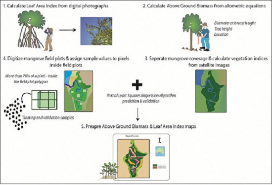
2. Data and Methods
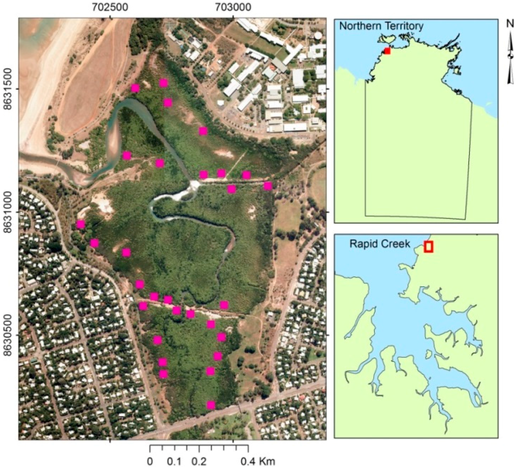
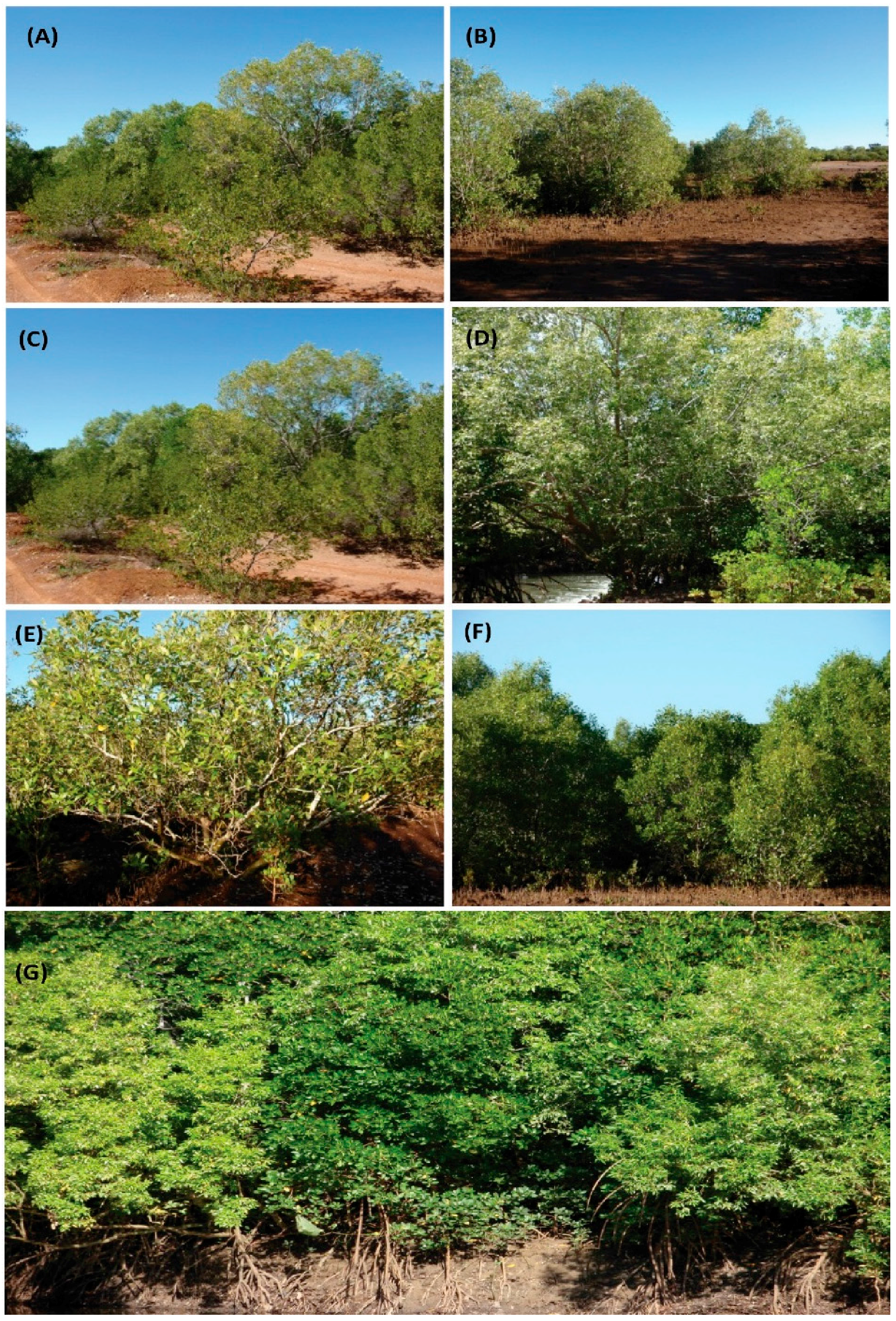
2.1. Study Area
2.2. Field Sampling, Satellite Data and Predictor Variables
2.2.1. Remotely-Sensed Data and Predictor Variables
2.2.2. Estimating the Leaf Area Index
2.2.3. Estimating the Above Ground Biomass
2.3. Predicting LAI and AGB
2.4. Accuracy Assessment
3. Results
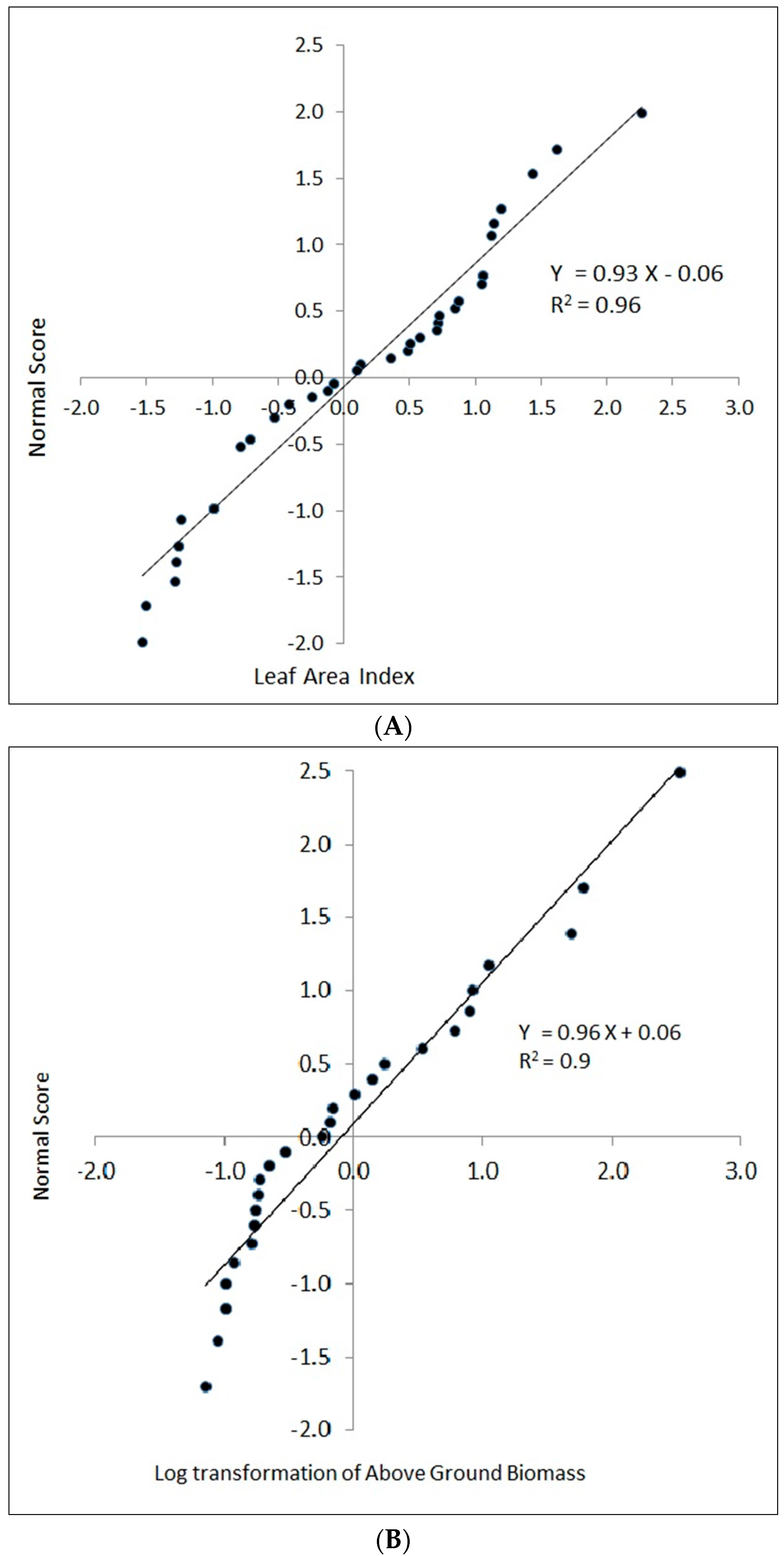
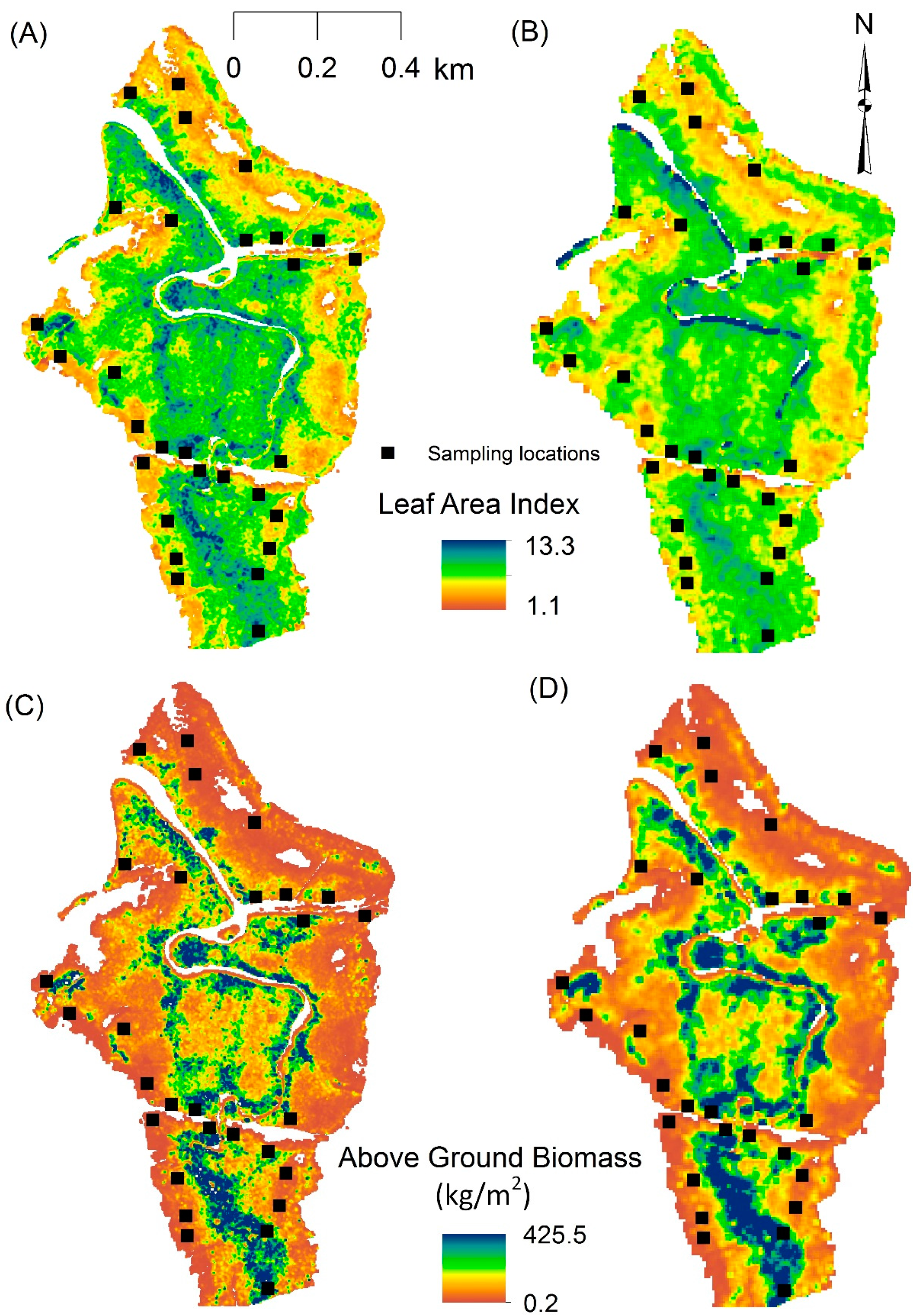
3.1. Predicting AGB and LAI
3.2. Accuracy Assessment
4. Discussion
4.1. Predicting LAI
4.2. Predicating AGB
5. Conclusions and Recommendations
Acknowledgments
Author Contributions
Conflicts of Interest
References
- Food and Agriculture Organisation of the United Nations (FAO). The World’s Mangroves 1980–2005; Food and Agriculture Organisation of the United Nations: Rome, Italy, 2007. [Google Scholar]
- Bouillon, S.; Rivera-Monroy, V.H.; Twilley, R.R.; Kairo, J.G. Mangroves. In The Management of Natural Coastal Carbon Sinks; Laffoley, D., Grimsditch, G., Eds.; International Union for Conservation of Nature and Natural Resources (IUCN): Gland, Switzerland, 2009. [Google Scholar]
- Wilkie, M.L.; Fortuna, S.; Forestry Department; FAO. Status and Trends in Mangrove Area Extent Worldwide; FAO: Rome, Italy, 2003; Available online: www.fao.org/docrep/007/j1533e/J1533E02.htm (accessed on 17 August 2016).
- Fu, W.; Wu, Y. Estimation of aboveground biomass of different mangrove trees based on canopy diameter and tree height. Procedia Environ. Sci. 2011, 10, 2189–2194. [Google Scholar] [CrossRef]
- Komiyama, A.; Ong, J.E.; Poungparn, S. Allometry, biomass, and productivity of mangrove forests: A review. Aquat. Bot. 2008, 89, 128–137. [Google Scholar] [CrossRef]
- Metcalfe, K.; Franklin, D.C.; McGuinness, K.A. Mangrove litter fall: Extrapolation from traps to a large tropical macrotidal harbour. Estuar. Coast. Shelf Sci. 2011, 95, 245–252. [Google Scholar] [CrossRef]
- Anaya, J.A.; Chuvieco, E.; Palacios-Orueta, A. Aboveground biomass assessment in Colombia: A remote sensing approach. For. Ecol. Manag. 2009, 257, 1237–1246. [Google Scholar] [CrossRef]
- Roy, P.S.; Ravan, S.A. Biomass estimation using satellite remote sensing data—An investigation on possible approaches for natural forest. J. Biosci. 1996, 21, 535–561. [Google Scholar] [CrossRef]
- Eckert, S. Improved forest biomass and carbon estimations using texture measures from WorldView-2 satellite data. Remote Sens. 2012, 4, 810–829. [Google Scholar] [CrossRef]
- Ahamed, T.; Tian, L.; Zhang, Y.; Ting, K.C. A review of remote sensing methods for biomass feedstock production. Biomass Bioenergy 2011, 35, 2455–2469. [Google Scholar] [CrossRef]
- Satyanarayana, B.; Mohamad, K.A.; Idris, I.F.; Husain, M.-L.; Dahdouh-Guebas, F. Assessment of mangrove vegetation based on remote sensing and ground-truth measurements at Tumpat, Kelantan delta, east coast of Peninsular Malaysia. Int. J. Remote Sens. 2011, 32, 1635–1650. [Google Scholar] [CrossRef]
- Simard, M.; Rivera-Monroy, V.H.; Mancera-Pineda, J.E.; Castañeda-Moya, E.; Twilley, R.R. A systematic method for 3d mapping of mangrove forests based on shuttle radar topography mission elevation data, ICEsat/GLAS waveforms and field data: Application to Ciénaga Grande de Santa Marta, Colombia. Remote Sens. Environ. 2008, 112, 2131–2144. [Google Scholar] [CrossRef]
- Mitchard, E.T.A.; Saatchi, S.S.; White, L.J.T.; Abernethy, K.A.; Jeffery, K.J.; Lewis, S.L.; Collins, M.; Lefsky, M.A.; Leal, M.E.; Woodhouse, I.H.; et al. Mapping tropical forest biomass with radar and spaceborne LiDAR in Lope National Park, Gabon: Overcoming problems of high biomass and persistent cloud. Biogeosciences 2012, 9, 179–191. [Google Scholar] [CrossRef]
- Green, E.P.; Mumby, P.J.; Edwards, A.J.; Clark, C.D.; Ellis, A.C. Estimating leaf area index of mangrove from satellite data. Aquat. Bot. 1997, 58, 11–19. [Google Scholar] [CrossRef]
- Kamal, M.; Phinn, S.; Johansen, K. Assessment of multi-resolution image data for mangrove leaf area index mapping. Remote Sens. Environ. 2016, 176, 242–254. [Google Scholar] [CrossRef]
- Zhu, Y.; Liu, K.; Liu, L.; Wang, S.; Liu, H. Retrieval of mangrove aboveground biomass at the individual species level with WorldView-2 images. Remote Sens. 2015, 7, 12192–12214. [Google Scholar] [CrossRef]
- Clough, B.F.; Ong, J.E.; Gong, W.K. Estimating leaf area index and photosynthetic production in canopies of the mangrove Rhizophora apiculata. Mar. Ecol. Prog. Ser. 1997, 159, 285–292. [Google Scholar] [CrossRef]
- Green, E.; Clark, C. Assessing mangrove leaf area index and canopy closure. In Remote Sensing Handbook for Tropical Coastal Management (Extracts); Edwards, A.J., Ed.; UNESCO: Paris, France, 2000. [Google Scholar]
- Komiyama, A.; Poungparn, S.; Kato, S. Common allometric equations for estimating the tree weight of mangroves. J. Trop. Ecol. 2005, 21, 471–477. [Google Scholar] [CrossRef]
- Perera, K.A.R.S.; Amarasinghe, M.D. Carbon partitioning and allometric relashionships between stem diameter and total organic carbon (TOC) in plant components of Bruguiera gymnorrhiza (L.) Lamk. and Lumnitzera racemosa willd. in a Microtidal Basin Estuary in Sri Lanka. Int. J. Mar. Sci. 2013, 3, 72–78. [Google Scholar]
- Heenkenda, M.K.; Joyce, K.E.; Maier, S.W.; Bartolo, R. Mangrove species identification: Comparing WorldView-2 with aerial photographs. Remote Sens. 2014, 6, 6064–6088. [Google Scholar] [CrossRef]
- Duke, N.C. Australia’s Mangroves—The Authoritative Guide to Australia’s Mangrove Plants; University of Queensland: Brisbane, Australia, 2006; p. 200. [Google Scholar]
- Wightman, G. Mangrove Plant Identikit for North Australia’s Top End; Greening Australia: Darwin, Australia, 2006; p. 64. [Google Scholar]
- Rouse, J.W., Jr.; Haas, R.H.; Schell, J.A.; Deering, D.W. Monitoring vegetation systems in the great plains with Erts. In Third Earth Resources Technology Satellite-1 Symposium; NASA: Washington, DC, USA, 1974; pp. 309–317. [Google Scholar]
- Barnes, E.M.; Clarke, T.R.; Richards, S.E.; Colaizzi, P.D.; Haberland, J.; Kostrzewski, M.; Waller, P.; Choi, C.; Riley, E.; Thompson, T.; et al. Coincident detection of crop water stress, nitrogen status and canopy density using ground-based multispectral data. In Proceedings of the Fifth International Conference on Precision Agriculture, Bloomington, MN, USA, 16–19 July 2000.
- Li, X.; Zhang, Y.; Bao, Y.; Luo, J.; Jin, X.; Xu, X.; Song, X.; Yang, G. Exploring the best hyperspectral features for lai estimation using partial least squares regression. Remote Sens. 2014, 6, 6221–6241. [Google Scholar] [CrossRef]
- Gitelson, A.A.; Kaufman, Y.J.; Merzlyak, M.N. Use of a green channel in remote sensing of global vegetation from EOS-MODIS. Remote Sens. Environ. 1996, 58, 289–298. [Google Scholar] [CrossRef]
- Mutanga, O.; Adam, E.; Cho, M.A. High density biomass estimation for wetland vegetation using WorldView-2 imagery and random forest regression algorithm. Int. J. Appl. Earth Obs. Geoinf. 2012, 18, 399–406. [Google Scholar] [CrossRef]
- Qi, J.; Chehbouni, A.; Huete, A.R.; Kerr, Y.H.; Sorooshian, S. A modified soil adjusted vegetation index. Remote Sens. Environ. 1994, 48, 119–126. [Google Scholar] [CrossRef]
- Macfarlane, C.; Hoffman, M.; Eamus, D.; Kerp, N.; Higginson, S.; McMurtrie, R.; Adams, M. Estimation of leaf area index in eucalypt forest using digital photography. Agric. For. Meteorol. 2007, 143, 176–188. [Google Scholar] [CrossRef]
- Pekin, B.; Macfarlane, C. Measurement of crown cover and leaf area index using digital cover photography and its application to remote sensing. Remote Sens. 2009, 1, 1298–1320. [Google Scholar] [CrossRef]
- Heenkenda, M.K.; Joyce, K.E.; Maier, S.W.; Bruin, S.D. Quantifying mangrove chlorophyll from high spatial resolution imagery. ISPRS J. Photogramm. Remote Sens. 2015, 108, 234–244. [Google Scholar] [CrossRef]
- Lui, J.; Pattey, E. Retrieval of leaf area index from top-of-canopy digital photogrpahy over agricultural crops. Agric. For. Meteorol. 2010, 150, 1485–1490. [Google Scholar]
- Walker, J.; Tunstall, B.R. Field Estimation of Foliage cover in Australian Woody Vegetation; CSIRO Institute of Biological Resources: Canberra, Australia, 1981; p. 18. [Google Scholar]
- Perera, K.A.R.S.; Amarasinghe, M.D.; Somaratna, S. Vegetation structure and species distribution of mangroves along a soil salinity gradient in a micro tidal estuary on the North-Werstern coast of Sri Lanka. Am. J. Mar. Sci. 2013, 1, 7–15. [Google Scholar]
- Breda, N.J.J. Ground-based measurements of leaf area index: A review of methods, instruments and current controversies. J. Exp. Bot. 2003, 54, 2403–2417. [Google Scholar] [CrossRef] [PubMed]
- Chen, J.M. Optically-based methods for measuring seasonal variation of leaf area index in boreal conifer stands. Agric. For. Meteorol. 1996, 80, 135–163. [Google Scholar] [CrossRef]
- Chen, J.M.; Rich, P.M.; Gower, S.T.; Norman, J.M.; Plummer, S. Leaf area index of boreal forests: Theory, techniques, and measurements. J. Geophys. Res. 1997, 102, 29429–29443. [Google Scholar] [CrossRef]
- Bai, L. The Colour of Mud: Blue Carbon Storage in Darwin Harbour; Charles Darwin University: Darwin, Australia, 2012. [Google Scholar]
- Comley, B.W.T.; McGuinness, K.A. Above-and below-ground biomass, and allometry, of four common Northern Australian mangroves. Aust. J. Bot. 2005, 53, 431–436. [Google Scholar] [CrossRef]
- Clough, B.F.; Scott, K. Allometric relationships for etimating above-ground biomass in six mangroves species. For. Ecol. Manag. 1989, 27, 117–127. [Google Scholar] [CrossRef]
- Carrascal, L.M.; Galvan, I.; Gordo, O. Partial least squares regression as an alternative to current regression methods used in ecology. Oikos 2009, 118, 681–690. [Google Scholar] [CrossRef]
- Wang, F.; Huang, J.; Lou, Z. A comparison of three methods for estimating leaf area index of paddy rice from optimal hyperspectral bands. Precis. Agric. 2011, 12, 439–447. [Google Scholar] [CrossRef]
- Mevik, B.; Wehrens, R. The pls pckage: Principal component and partial least squares regression in R. J. Stat. Softw. 2007, 18, 1–24. [Google Scholar] [CrossRef]
- Hastie, T.; Tibshirani, R.; Friedman, J. Linear methods for regression. In The Elements of Statistical Learning: Data Mining, Inference, and Prediction; Springer: New York, NY, USA, 2001; p. 533. [Google Scholar]
- Hijmans, R.J.; van Etten, J. Raster: Geographic Analysis and Modeling. R Package Version 2.2–31. Available online: http://CRAN.R-project.org/package=raster (accessed on 17 August 2016).
- Zheng, G.; Moskal, L.M. Retrieving leaf area index (LAI) using remote sensing: Theories, methods and sensors. Sensors 2009, 9, 2719–2745. [Google Scholar] [CrossRef] [PubMed]
- Laongmanee, W.; Vaiphasa, C.; Laongmanee, P. Assessment of spatial resolution in estimating leaf area index from satellite images: A case study with Avicennia marina plantations in Thaliland. Int. J. Geomat. 2013, 9, 69–77. [Google Scholar]
- Clough, B.F.; Dixon, P.; Dalhaus, O. Allometric relationships for estimating biomass in multi-stemmed mangrove trees. Aust. J. Bot. 1997, 45, 1023–1031. [Google Scholar] [CrossRef]
- Clough, B.F.; Andrews, T.J. Some ecophysiological aspects of primary production by mangroves in North Queensland. Wetlands 1981, 1, 6–7. [Google Scholar]
- Alongi, D.M. Present state and future of the world’s mangrove forests. Environ. Conserv. 2002, 29, 331–349. [Google Scholar] [CrossRef]


| Band | Spectral Range (nm) | Spatial Resolution (m) |
|---|---|---|
| Panchromatic | 447–808 | 0.5 |
| Coastal | 396–458 | 2 |
| Blue | 442–515 | |
| Green | 506–586 | |
| Yellow | 584–632 | |
| Red | 624–694 | |
| Red-edge | 699–749 | |
| NIR1 | 765–901 | |
| NIR2 | 856–1043 |
| Vegetation Index | Band Relationship | Source |
|---|---|---|
| Normalized Difference Vegetation Index (NDVI) | Rouse et al. [24] and Ahamed et al. [10] | |
| Normalized Difference Red Edge index (NDRE) | Ahamed et al. [10] and Barnes et al. [25] | |
| Green Normalized Difference Vegetation Index (GNDVI) | Ahamed et al. [10], Li et al. [26] and Gitelson et al. [27] | |
| Green Normalized Difference Vegetation Index 2 (GNDVI2) | Mutanga et al. [28] | |
| Normalized Difference Vegetation Index 2 (NDVI2) | Mutanga et al. [28] | |
| Normalized Difference Red Edge index 2 (NDRE2) | Mutanga et al. [28] | |
| Renormalized Vegetation Index (RDVI) | Li et al. [26] | |
| Ratio Vegetation Index (RVI) | Li et al. [26] | |
| Modified Soil Adjusted Vegetation Index (MSAVI) | Qi et al. [29] |
| Mangrove Species | B0 | B1 | Study |
|---|---|---|---|
| Avicennia marina | −0.511 | 2.113 | Comley and McGuinness [40] |
| Bruguiera exaristata | −0.643 | 2.141 | Comley and McGuinness [40] |
| Ceriops tagal | −0.7247 | 2.3379 | Clough and Scott [41] |
| Lumnitzera racemosa | 1.788 | 2.529 | Perera and Amarasinghe [20] |
| Rhizophora stylosa | −0.696 | 2.465 | Comley and McGuinness [40] |
| Sonneratia alba | −0.634 | 2.248 | Bai [39] |
| Excoecaria agallocha var. ovalis | −0.634 | 2.248 | Bai [39] |
| Biophysical Variable | RMSE | Correlation Coefficient | ||
|---|---|---|---|---|
| Spatial resolution | 2 m | 5 m | 2 m | 5 m |
| Above ground biomass (AGB) | 2.2 kg/m2 | 2.0 kg/m2 | 0.4 | 0.8 |
| Leaf area index (LAI) | 0.75 | 0.78 | 0.7 | 0.8 |
© 2016 by the authors; licensee MDPI, Basel, Switzerland. This article is an open access article distributed under the terms and conditions of the Creative Commons Attribution (CC-BY) license (http://creativecommons.org/licenses/by/4.0/).
Share and Cite
Heenkenda, M.K.; Maier, S.W.; Joyce, K.E. Estimating Mangrove Biophysical Variables Using WorldView-2 Satellite Data: Rapid Creek, Northern Territory, Australia. J. Imaging 2016, 2, 24. https://0-doi-org.brum.beds.ac.uk/10.3390/jimaging2030024
Heenkenda MK, Maier SW, Joyce KE. Estimating Mangrove Biophysical Variables Using WorldView-2 Satellite Data: Rapid Creek, Northern Territory, Australia. Journal of Imaging. 2016; 2(3):24. https://0-doi-org.brum.beds.ac.uk/10.3390/jimaging2030024
Chicago/Turabian StyleHeenkenda, Muditha K., Stefan W. Maier, and Karen E. Joyce. 2016. "Estimating Mangrove Biophysical Variables Using WorldView-2 Satellite Data: Rapid Creek, Northern Territory, Australia" Journal of Imaging 2, no. 3: 24. https://0-doi-org.brum.beds.ac.uk/10.3390/jimaging2030024