1. Introduction
Soil structure is the term given to the arrangement of differently-sized mineral particles and organic material into larger, more complex arrangements in the soil. Good structure improves soil hydraulic properties, allows air and roots to move freely through the soil and provides a suitable habitat for microbes, fungi and soil fauna. Poor structure implies smaller overall pore space, reduced numbers of large pores and a lack of internal spaces for the physical and chemical protection of organic matter and living organisms. Soil texture is the proportional distribution of particles of different sizes, commonly divided into sand (>50 μm), silt (2–50 μm) and clay (<2 μm) particles (these size range definitions vary in the literature). Both soil texture and structure have important impacts on several factors including plant growth, nutrient availability and soil hydrology.
Assessment of soil structure and texture is an important component of determining physical condition and degradation of soils. The soil structure and its impact on soil health and resilience to disturbance can be measured using a number of different approaches, including physical and visual, while estimates of soil texture are normally carried out by hand or using a number of laboratory approaches. It was demonstrated [
1] that the geometric characteristics of soil pores varied under different levels of compaction and structural damage. Visual soil assessment approaches give results that in many cases link closely to direct physical measurements of structure-related soil parameters [
2].
It has been pointed out [
3] that laboratory-based assessment of soil sample structure does not produce a fair indication of soil structure, and that soil structure does not lend itself to quantification. The same is not true of soil texture, which can be measured directly in the laboratory but which still relies on fairly subjective “hand-texturing” approaches in the field. One alternative could be to determine if image analysis of the visible structure of soils can lead to automated soil structure assessment in the field. A clear statistical link has been drawn [
4] between the spatial organisation and forms of soil components at the microscopic scale, and the character and stability of soil structure. If this is also true at larger scales such as those visible to digital cameras, then this automated image analysis might be possible.
Changes in soil micromorphology, specifically relating to pore size distribution and hence to soil structure, can be detected following changes to tillage practices [
5]. The same management of soils with different textural proportions (sand, silt, clay) will not result in the same soil structure. Therefore, it is also worthwhile investigating whether soil texture can be linked to image analysis of soil profiles, and estimated using the same approaches.
Mineralogical analysis may traditionally have provided better information on soil structure at microscopic scales than micromorphological analysis [
6]. However, improvements in characterising 2D image of complex systems such as soil may now mean that image analysis is on an equal footing with mineralogy in this area. Early work on digital information of pore structure (e.g., [
7,
8]) demonstrated links between soil structure and image structure, but required careful preparation of soil samples (i.e., impregnation with epoxy resin, sawing, polishing).
A study by [
9] demonstrated a link between morphological measurements of soil structure in the field and soil compaction. Visualisation of soil aggregate structure and pore size/connectivity using X-ray tomography reveals links between structural parameters related to bulk density and water movement [
10]. It was also demonstrated [
11] that the use of 2D tomography for assessing soil structure properties could provide sufficient information to assess structural quality.
This implies that soil structural assessment, including information about bulk density, can be automated through appropriate characterisation of photographs of soil profiles. The term “soil profile” here is taken to mean a vertical section of the soil, not the description of the sequence and character of the individual soil horizons, as it is sometimes taken to mean.
An approach has been described [
12] for visual assessment of soil structure that gives a numerical score to the structure. The soil features described in [
12] are amenable to visual discrimination, implying that a direct estimate of structural parameters may be possible. The benefit to farmers and other land managers of a rapid, low-cost method of assessing soil structure and soil degradation is emphasised in [
13].
The Visual Evaluation of Soil Structure (VESS) approach developed by [
12] (which was developed for agricultural soils commonly found in northern Europe) can also be applied successfully to Oxisols and potentially other tropical soils under different land use systems [
14] and to tropical soils under no-tillage agricultural systems [
15]. Arguably, a single method of automated soil structure assessment could potentially be applied in many parts of the world and to soils under many different management systems.
Investigation between visually measurable pore-structure attributes and levels of compaction show clear links that imply the ability to measure soil structure from digital imagery with mathematically defined parameters [
16]. A correlation was also shown [
17] between visual soil structure assessment scoring and the slope of the line between soil wetness and penetration resistance. This demonstrated a clear link between visual assessment scoring and physically-relevant soil structure measurements.
An assessment of different methods for visually assessing soil structure by [
18] showed that many approaches gave similar results and linked closely to shape and size of aggregates. These aggregates are visible and may be amenable to detection through image analysis approaches. This is an approach that has similarities to the method of [
12] and that indicates that aggregate size in particular is something that links both visual assessment and structure in soils.
Several methods exist for field-based assessment of soil structure, including a number that rely on visual interpretation [
19]. The VESS approach of [
12] by Bruce Ball, however, provides an approach for determining soil structure visually, and provides information that relates well to measurements from more instrument-reliant approaches for determining soil physical structure [
20].
Our aim is to show that in the last two and a half decades technological, statistical and modelling developments now mean that because it is possible to measure soil structure in the field rather than the laboratory, the quantification of soil structure and soil texture can now be achieved through image analysis directly linked to field-based soil structure assessment parameters and environmental conditions. We make extensive use of Ball’s approach, including the numerical scoring system and an image analysis method that utilises some of the descriptive features in this method.
Aggregate soil stability, a key parameter in soil structure, is influenced by a number of factors including climate, vegetation growth and soil management amongst other parameters (including soil texture) [
21]. Our assessment also includes several of these environmental factors, although it does not include land management history. In addition to structure, we estimate soil texture and drainage class using the same image analysis approach. Building on previous work linking soil colour and environmental factors to soil properties [
22], we also include LOI (Loss On Ignition) as an estimate of soil organic matter content, and soil pH. The overall method is related to current work in Digital Soil Mapping, which links spatial covariates (and occasionally remote sensing) to soil properties.
2. Materials and Methods
2.1. Soil Photography
Using a smartphone camera, a total of 103 images were acquired of topsoil (upper 30 cm) from sites across the north-east of Scotland. The sites were selected to provide variability in land cover, soil type, topography and parent material. Images were captured using an iPhone 2, with the site location also captured using the smartphone’s GPS. A colour correction card was placed within each shot to allow post-capture image colour correction, as soil colour is one of the factors that is considered important in mineralogy (and hence soil texture and structure). Natural lighting was used in each case, with no artificial sources. All photographs were taken under at least reasonable lighting conditions, without a flash being required. Colour correction was carried out using the approach described in [
23], and involved calculating the ratio between actual and expected RGB values at various intensity levels (0–255 in intensity bands 16 units across). This ratio was then applied to all pixels across the image that lay within the specific intensity level.
Figure 1 shows two examples of the images that were captured.
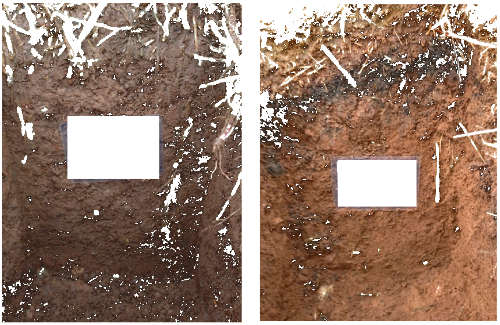
A total of 54 images were selected from the profile photographs taken during the NSIS2 (National Soil Inventory of Scotland 2007–2009) field campaign. The protocol for how these profiles was prepared and sampled is given in [
24] and two examples of the imagery are given in
Figure 2. The soil profile face was cleaned and photographed prior to sampling, and where possible the photograph was taken to clearly show the horizons and any important features of the soil. Clearly labelled signs with the Site ID (National Grid Intersect) were used in the photographs.
For the smartphone imagery, structural assessment was carried out in the field using the approach outlined by [
12] and detailed in the instructions available at the website of Scotland’s Rural College (SRUC). Prior to this work being carried out, the researchers involved spent time in the field testing the VESS approach and ensuring that they were confident in producing replicable estimates of structure. VESS scoring estimates were produced for the upper (top 15 cm) and lower (bottom 15 cm) of the exposed soil, to capture variation in structure with depth. For the NSIS2 imagery, the same procedure was carried out but only for the topsoil. In addition, the structural assessment for NSIS2 samples was only carried out on agricultural soils, meaning that the imagery selected is restricted to this land use/land cover class. Throughout this work, reference to soil structure is taken to mean assessment of the VESS score.
Each of the soil samples was analysed for sample size according to the specified ranges (<2 μm—clay; 2–50 μm—silt; >50 μm—sand). This analysis was carried out using a Mastersizer 2000 (Malvern Instruments). The same procedure was applied to samples relating to both types of imagery. Loss On Ignition (LOI) was carried out for each sample at 450 °C for 24 h in a muffle furnace. Bulk density was calculated from the volume and mass of an oven-dried core, dried at 105 °C for 24 h. pH was measured using a 0.01 M solution of CaCl
2. Structure was assessed in the field using the method described by [
12] and involves a manual and visual assessment of how easily the soil breaks up and the shapes/sizes of the soil fragments. Drainage is an assessment of the drainage characteristics of the whole soil profile, and so depends also on features below the topsoil; values given include very poor (1); poor (2); imperfect (3); moderate (4) and freely-draining (5).
2.2. Image Analysis
Each soil image (lossless JPEG format) was converted to digital numbers and stored as three arrays (one each for red, green and blue pixel values) with values ranging from 0 to 255. Following colour correction (on the smartphone imagery—colour correction cards were not used in the NSIS2 protocol), non-soil pixels were removed by selection of pixels with high ratios of green or blue to red (ratio greater than 1), or that had been identified as belonging to the colour correction card.
Figure 3 shows two examples of this pixel elimination process using the same images as in
Figure 1, with the resulting images containing only pixels identified as belonging to soil or plant roots.
The average colour ratios for the upper and lower half of each image were then determined, with a value given to the mean proportion of each total pixel intensity (i.e., not the absolute, but the proportion of the summed RGB values) that was red, blue or green. Each image was therefore represented by six values (mean R, mean G, mean B for top and bottom of image). These values have been found useful in estimating topsoil organic matter content [
22] and in estimating soil texture in ongoing unpublished work by this research group. Each image does not represent the same soil profile depth and so the upper and lower halves of the image are not representative of the same depths each time.
For structural assessment, a greyscale version of the image was derived by taking the average of the red, green and blue pixel values for each pixel. In order to assess the range of structures within each image, a moving window centred on the pixel of interest was passed over each pixel to normalise the intensity of that pixel in relation to its surroundings, followed by thresholding and boundary density counting. Pixels that had been removed due to colour or intensity thresholding were not included in this analysis. The following steps were carried out on each pixel of the greyscale image for a number of moving window sizes:
Identify the minimum (Min) and maximum (Max) pixel values within the moving window;
Normalise the target pixel value P0 within the moving window range, defining the new pixel value P1 as P1 = INT(256 × (P0 − Min)/(Max − Min)).
Following normalisation of each pixel, threshold the pixel value so that all values below 128 are set to 0, and all values equal to or above 128 are set to 255.
For each horizontal row of pixels in the image, calculate the number of boundaries between 0 and 255 for neighbouring pixels in any direction (soil pixels only). Divide this number by the number of soil pixels in the row.
In practice, identification of the minimum and maximum pixel values within the moving window was estimated by selecting 100 pixels at random within the moving window; this prevented the processing time from becoming prohibitive as the moving window size increased. It was assumed that selecting this number of pixels would provide a good estimation of the range of values within the moving window. The following moving window sizes were used: 1, 2, 4, 8, 16, 32, 64, 128 and 256 pixels. In each case, the moving window included all pixels within this distance in the x or y directions (i.e., a square window of side length 2N + 1, where N is the moving window size). For moving window sizes of 8 or less, all pixels were used as the total number of pixels in the window was less than 100.
The result of the above steps for each moving window size is to produce a set of images that represents the local granularity of the image at a number of scales. This local granularity was assumed to reflect the physical structure within the soil. Counting the proportion of boundaries between thresholded pixels gives an indication of the distribution of aggregates within the image. The boundary proportion value was recorded for all rows in the image and average values were recorded for the upper and lower half of the image (discounting those pixels that contained non-soil pixels, the colour correction card or that were within one moving window size of it).
2.3. Environmental Characteristics
The GPS-recorded location of each sample site was used to determine a number of environmental characteristics. The parameters here were derived from a number of spatial datasets, including the following:
2.4. Modelling Soil Characteristics
An artificial neural network (ANN) model was used to estimate soil structural and texture parameters. The ANN was trained using 10-fold cross-validation. This method involves producing 10 subsamples of the training data, and 10 ANN models being developed, each trained with 9 out of the 10 randomly-generated subsamples and validated with the “missing” subsample. Each ANN was validated using a different subsample. The structure of the ANN used 104 inputs, including the 80 derived from environmental parameters and the 24 derived from image analysis (textural measurement at nine different moving window sizes, red green and blue colour average for both upper and lower image).
A single hidden layer in each ANN contained 10 nodes. There were 2 output nodes for the smartphone imagery (LOI and VESS structure each normalised in the range 0 to 1) and 7 for the NSIS2 imagery (drainage class, LOI, bulk density, sand, silt, clay and pH each normalised to the range 0 to 1). Each ANN was trained using the backpropagation gradient descent algorithm with a learning rate of 0.05. Training was carried out over 20,000 training steps each with random input selection, and validated every 1000 training steps to allow optimal training to be selected.
In addition to the above ANN design, we also tested the model using information derived only from (A) location information (80 inputs, same hidden node and output architecture) and (B) image analysis (24 inputs, same hidden node and output architecture). The same training regime was also used as for above. These secondary models were developed to allow us to determine the relative importance of spatial covariates or image characteristics in the input model. It was anticipated that image analysis would be more important for soil structural assessment and that spatial covariates would be more important in estimating soil texture because: (1) the image resolution is not sufficient to capture particles within the necessary size range to describe soil texture; and (2) the spatial covariates used would have less impact on soil structure than local management conditions.
In terms of estimating drainage, LOI and pH, it was also suspected that the spatial covariates would provide more useful information than image analysis, as visual examination of soil profiles does not allow an obvious way of estimating these while environmental conditions are known to have a strong influence on these soil characteristics.
Statistical evaluation of model performance was carried out using a number of metrics. These included r
2, RMSE (Root Mean Square Error), MAE (Mean Absolute Error), RPD (Ratio of Performance to Deviation) and RPIQ (Ratio of Performance to Interquartile distance). RPD is the ratio of standard error of prediction to the standard deviation of the variable’s actual values, and is commonly used to provide an indication of model quality, with values greater than 2 often being taken to indicate good model performance. However, [
30] showed that RPD is closely related to r
2, particularly for normally distributed data and large sample size, with the relationship RPD = (1 − r
2)
−0.5 at this limit. They proposed instead that RPIQ should be used, as described by [
31], as it better represents the spread of values in a dataset. The values given of RPIQ are usually within a factor of 2 of RPD values, and so it is possible (but not to be encouraged) to take RPIQ values of greater than 2 to indicate good model performance.
For structure and drainage, which are categorical variables rather than being continuous, the use of r2 and some of the other statistical metrics is acknowledged to be suspect; the use of these is only really appropriate for continuous variables. A more appropriate measure in this case is one of several possible pseudo-r2 regression methods. However, as we are dealing here with variables that have multiple possible values rather than being binary, it was felt that the standard r2 calculation could in this case be used as a metric of performance.
4. Discussion
In absolute terms, none of the soil variables was estimated with an accuracy that would enable their estimation in the field to replace laboratory or field analysis by a trained observer. None achieved an RPD of greater than 2 (a value commonly taken to indicate “good” estimation) even with the best model. Drainage and clay percentage had RPD values of less than 1.5. Clay in particular had extremely low RPD values and did not follow the relationship given in [
30] linking this with r
2. The distribution of values for clay may have affected this result, as it did not have a normal distribution, and the values given for RPIQ were also below 2. However, for estimating values for land management decision making or rapid condition assessment, the levels of accuracy achieved (as expressed by RMSE and MAE) are sufficient to give a “low/medium/high” estimate of every variable estimated.
The best model developed for estimating VESS structure gives an RMSE value of less than 1, and so if given a value of 2, for example, the user could be confident that the soil examined was not a 4 or 5. For pH similarly, the user can safely assume that the value given is within 1 pH unit of the actual value. This level of confidence is suitable for calculating liming rates. Drainage, bulk density and soil texture parameters are given with sufficient accuracy to detect compaction or evaluate candidate management options. Drainage in particular is an indication of the whole soil profile’s drainage characteristics and so being able to make even a coarse assessment using information only from the upper soil is potentially very useful.
The neural network models used spatial covariates for Scotland’s landscape. As such, the exact models would provide poorer performance if applied elsewhere, particularly in geographical regions with significantly different climate, soil or vegetation types. In order to achieve corresponding levels of accuracy, models would need to be developed that were specific to the regions of interest, which for many parts of the world may be difficult due to a lack of mapped information. The methodology used here is strongly dependent on available data, both from soil surveys and from spatial datasets with appropriate accuracy and resolution. As such, while globally applicable it would not provide the same level of accuracy in parts of the world that were poorly surveyed and mapped, particularly if these areas are spatially heterogeneous. This is an ongoing challenge for all areas of soil mapping, particularly in the digital age. There is also a distinction to be made between natural/seminatural and cultivated soils, where management is likely to play a much stronger role in soil characteristics. Management was not a factor included in this work, and would be necessary to include for some soils, particularly where agriculture has been present for hundreds of years.
The models are relatively small and computationally inexpensive, and could be implemented within a smartphone app quite easily. An existing app that provides a template for this is the SOCIT app, which estimates topsoil organic matter content for mineral soils in Scotland. This app links to similar spatial covariates as are used in this work, by sending the topsoil image with user coordinates to a server at the James Hutton Institute where the necessary large datasets are held. One limitation that we cannot improve on within our own work is the positional accuracy achieved by smartphones and tablets equipped with GPS; depending on the device and the quality of the signal acquired, this ranges between approximately 5 and 50 m. In linking positional information to spatial covariates, we therefore must be aware that in landscapes that are spatially heterogeneous, positional inaccuracy may increase error rates for variables of interest.
Ongoing research in this area indicates that LOI, pH and bulk density in particular can be estimated with better accuracy than demonstrated here, if sufficient data is provided. Spectroscopy in particular can provide good estimates of many soil variables non-destructively. However, this work was intended to produce a method of estimating all of the variables of interest from a dataset of available imagery, reducing the need to gather additional information. We intend to expand the resource of available data and imagery to produce a more robust and accurate model capable of improving on the levels of accuracy demonstrated here. The final objective of this work is to produce an app that can provide rapid assessments of several topsoil characteristics for Scottish soils.
The working hypothesis, that information derived from imagery would be more important for estimating structure while spatial covariates would provide more useful for estimating the other parameters, was largely borne out. Structure is no doubt affected by environmental conditions but is also strongly influenced by management, which is spatially variable but was not incorporated as an input to the modelling. Characteristics relevant to structure are often visible (e.g., cracking, solid blocky peds, macropores), implying that with appropriate image metrics, it should be possible to measure indicators of these and other structural features.
We also saw that in addition to structure, bulk density modelling was strongly affected by removing the imagery data from the modelling. It is possible that image features indicative of densely-packed soils are correlated to the measured image characteristics, and this deserves further study.
Soil texture variable estimation was approximately equal for the two data types, while LOI and pH appear to more strongly linked to spatial covariates. It is not surprising that pH is more strongly linked to environmental character than image metrics, as the visual appearance of topsoil does not often provide clues to pH levels even to trained field surveyors. Local conditions such as vegetation or parent material however are known to have a strong influence on soil pH levels.
An unexpected result was that the drop in model performance when removing one data type was not as great as expected for any of the variables modelled. It appears that both image characteristics and environmental conditions can contribute useful information to all variables that we studied here. It is possible that the characteristics measured in the imagery are in some way connected to the environmental conditions at each site, which would make it harder than expected to discriminate between the relative importance of different inputs. For example, particularly wet and cold climate conditions could result in soils with a specific visual appearance, which would be reflected in the image analysis data produced.
Further work on the linkages between environmental conditions and the visual appearance of the soil would help in resolving this. In order to achieve this, it is necessary to further investigate the possible image metrics that could be measured, as those selected for this work may not be the most appropriate. This would also benefit any further modelling work in the area of estimating soil characteristics from soil profile image analysis. It would also help to improve the spatial resolution of some of the parameters, particularly topography, as the current 100 m resolution that was used in this work does not reflect the spatial heterogeneity of Scotland’s landscape in some areas, particularly the fragmented mountainous regions in the north and west. Current work on digital soil mapping at the James Hutton Institute includes the development of a range of 10 m resolution topography products, to be incorporated into further research. As mentioned above, this will correspond to the approximate resolution achieved by current smartphone/tablets equipped with GPS.
Currently, we are developing a collection of imagery for Scottish soils that covers a wider range of soils and environmental conditions than was used in this work. We are also working on the identification of image analysis metrics that provide better representation of the soil under field conditions.


