
Measuring Leaf Thickness with 3D Close-Up Laser Scanners: Possible or Not?


Institue of Geodesy and Geoinformation, University of Bonn, Nussallee 17, 53115 Bonn, Germany
*
Author to whom correspondence should be addressed.
J. Imaging 2017, 3(2), 22; https://0-doi-org.brum.beds.ac.uk/10.3390/jimaging3020022
Submission received: 30 March 2017
/
Revised: 29 May 2017
/
Accepted: 10 June 2017
/
Published: 15 June 2017
(This article belongs to the Special Issue 2D, 3D and 4D Imaging for Plant Phenotyping)
Abstract
:Measuring the 3D shape of plants for phenotyping purposes using active 3D laser scanning devices has become an important field of research. While the acquisition of stem and root structure is mostly straightforward, extensive and non-invasive measuring of the volumetric shape of leaves, i.e., the leaf thickness, is more challenging. Therefore, the purpose of this paper is to examine whether the leaf thickness is measurable using a high precision industrial laser scanning system. The study comprises a metrological investigation of the accuracy of the laser scanning system with regards to thickness measurements as well as experiments for leaf thickness measurements using several leaves of three different types of crop. The results indicate that although the measuring system is principally able to measure thicknesses of about 74 m with statistical certainty, the leaf thickness is not measurable accurately. The reason for this can be attributed to the measurable penetration depth of the laser scanner combined with the variation of the angle of incidence. These effects cause systematic uncertainties and significant variations of the derived leaf thickness.
1. Introduction
Analyzing the 3D shape of plants to understand the plant’s structural response to its environment has become an important tool for plant phenotyping [1]. Three-dimensional measurements are performed on different scales [2] using active and passive imaging systems resulting in 3D point clouds representing the plant’s surface geometry. From these point clouds, phenotypic parameters such as leaf area [3], leaf area index [4], leaf angle [4], stem height [3] or biomass [5,6,7] are derived. Most of these parameters need accurate and highly resolved 3D point clouds in order to derive accurate phenotypic parameter values. For example, directly measuring the above-ground biomass of plants is extremely challenging. Commonly, the biomass is estimated indirectly using a function obtained by comparing non-invasive measuring techniques to destructive methods, e.g., biomass compared to pixel area using 2D cameras [8] or biomass compared to mean reflection height using a laser scanning system [5]. Measuring the biomass directly requires a volumetric representation of the whole plant, i.e., the roots, the stem and the leaves. Regarding the excavated roots and the stem, different approaches using terrestrial laser scanners [6] or high precision close-up laser scanning systems [3,7] exist. Thereby, the three-dimensional structure of the stems or roots is measured with laser sensors and the phenotypic parameters are derived using a mesh representation [6] or a cylinder fitting [3].
However, measuring the volumetric shape of a leaf is a lot more challenging. Due to the fact that most of the leaves provide a thickness of only a few tenths of a millimeter, the measuring system has to be more accurate in order to derive the leaf thickness with statistical certainty. Commonly, leaf thickness is measured for selected locations using either tactile measurements such as analog thickness gauges [9] and specially developed displacement sensors [10] or microscopes equipped with a coherent laser measuring system [11,12]. Consequently, these leaf thickness measurements are mostly invasive and only pointwise. Using a laser scanning system would provide non-invasive and extensive leaf thickness measurements for the whole leaf area. However, recent research has indicated that the interaction of the laser and the plant surface is not negligible and may impact the accuracy of laser-based measuring systems [13,14].
Therefore, the aim of this study is to answer the questions of whether it is possible to measure the thickness of crop leaves accurately using a high precision industrial laser scanning system and, if it is, which measuring setup is the most accurate one. This fundamental research comprises a theoretical assessment of the measurement process as well as metrological investigations of the laser scanning system. The latter ones are separated into two parts: a metrological investigation of the accuracy of thickness measurements using certified length and thickness gauges and an application study with three different types of crop.
This paper is structured as follows. Section 2 introduces the basics of leaf thickness measurements comprising an introduction of the measuring system and its sensors (Section 2.1) as well as an overview of its uncertainties (Section 2.2). Based on this, an optimized measuring setup for thickness measurements is suggested in Section 2.3. Metrological investigations on the empirical accuracy of thickness measurements based on gauges are illustrated in Section 3. In Section 4, the thickness of crop leaves is derived and the results are discussed in Section 5. Finally, all results are concluded in Section 6.
2. Basics of Leaf Thickness Measurements Using a Close-Up Laser Scanning System
This section outlines the basics of leaf thickness measurements using a laser scanning system comprising a coordinate measuring arm (CMA) and a close-up 2D laser triangulation sensor (LTS). Therefore, each component of the measuring system as well as the measuring setup is described. Furthermore, possible sources of measuring uncertainties are characterized with regard to the accuracy of leaf thickness measurements. Based on this, an optimized measuring setup is proposed that minimizes the uncertainties.
The reason for choosing this kind of measuring system is based on the accuracy requirements for deriving the leaf thickness. Under the assumption that leaves provide a thickness of a few tenths of a millimeter, the measuring system has to be more accurate to derive the thickness with statistical certainty. Non-invasive measuring technologies such as terrestrial laser scanners or photogrammetric approaches commonly do not fulfill these requirements. On the contrary, the combination of a CMA and a LTS has shown its applicability for plant phenotyping in the recent past [3,7,13,15,16]. It provides high accuracy and high spatial resolution together with high flexibility. Thus, the three-dimensional shape of a whole plant can be acquired without changing the position of the instrument.
2.1. Three-Dimensional Laser Scanning System
The measuring system comprises a 2D LTS and a 3D CMA so that complex geometries can be imaged in a nearly occlusion-free 3D point cloud [15].
Two-Dimensional Laser Triangulation Sensor
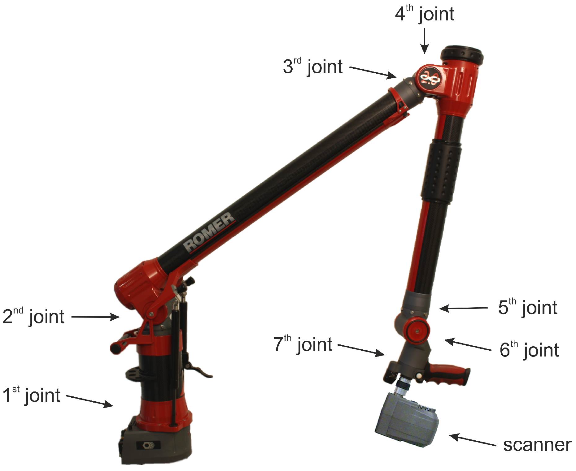
The appointed LTS is a ScanWorks-V5 from Perceptron company (Plymouth, MI, USA) (Figure 1). This sensor works according to the light-section method and principally measures the distance between the sensor’s reference and the object’s surface in two dimensions [17,18]. Therefore, a red laser line (wavelength: 660 nm) is emitted, backscattered from the object’s surface and imaged by two CCD (charge-coupled device)-arrays. From the position and the shape of the acquired laser line on the CCD-arrays, a 2D point cloud, also known as scan line, is calculated. This scan line consists of up to 7640 points with an averaged point-to-point distance of 14 m [19] in a field of view of approximate 110 mm × 105 mm (depth and width).
Due to the fact that the LTS only measures a 2D scan line, it has to be moved along the object’s surface. Consequently, the position and orientation of the LTS have to be measured with high accuracy in order to merge all scan lines into a 3D point cloud. To guarantee high accuracy as well as high flexibility, the scanner is combined with a CMA that is introduced in the subsequent section.
Coordinate Measuring Arm
The CMA used to track the position of the LTS is a seven DoF (Degree of Freedom) Infinite 2.0 from ROMER company (Wixom, MI, USA) (Figure 1). CMAs provide a special class of coordinate measuring machines (CMMs) where the 3D coordinates of the probe are calculated by a kinematic chain based on the Denavit–Hartenberg transformation [20,21]. Thereby, the probe coordinate is calculated by a consecutive transformation of local coordinate frames, located in the joints of the CMA. The parameters of these transformations, i.e., the kinematic calibration parameters, describe the geometrical construction of the CMA [22]. Each joint is equipped with a rotary encoder measuring the angular joint displacement. Applying these joint displacements and the calibration parameters in the kinematic chain, the 3D coordinate and orientation of the probe can be calculated.
2.2. Measurement Uncertainties of the Laser Scanning System
Principally, there are three possible sources of uncertainties when using the appointed laser scanning system:
- Uncertainties caused by the CMA,
- uncertainties caused by the LTS and
- uncertainties caused by the interaction of the laser and the leaf.
Uncertainties Caused by the CMA
The precision of each measuring point in the workspace, given as a maximum permissible error (mpe) by the manufacturer, is = 45 m [23]. However, measuring uncertainties of the CMA is mainly based on errors of the rotary encoders and deviations of the kinematic calibration parameters of the Denavit–Hartenberg transformation from the actual geometric construction [22]. Due to the high quality of the rotary encoders, systematic errors are negligible compared to the measuring noise, resulting in only small random errors of the 3D coordinate. On the contrary, the impact of deviations of the kinematic parameters on the point coordinate is much more significant. Due to the limited quality of the calibration procedure, the kinematic parameters do not reflect the actual geometric construction of the CMA, resulting in systematic errors of the 3D coordinate [22]. Furthermore, their impact on the point coordinate strongly depends on the joint configuration, i.e., if the CMA is moved a lot during the measurement process, the 3D probe coordinate will be less accurate. To illustrate the influence of this effect on thickness measurements, an empirical investigation of the CMA’s accuracy is performed in Section 3.1.
Uncertainties Caused by the LTS
On behalf of the manufacturer, the precision of each measured point in the scan line is = 12 m, guaranteed for the whole field of view [19]. However, uncertainties of the LTS mainly depend on an accurate adaption of the sensor properties, e.g., the exposure time to the optical characteristics of the object’s surface [18]. In order to reach the highest precision of the distance measurement, the exposure time has to be adjusted in a way to guarantee an optimal signal-to-noise ratio. An exposure time that is too short, i.e., an underexposed reception sensor, causes higher measuring noise, whereas an overexposure can cause systematic errors. These effects become particularly important if the optical characteristics of the object are not homogeneous and change during the measurement process.
Uncertainties Caused by the Interaction of the Laser and the Leaf
As shown in Paulus et al. [13], leaves are generally made of three different layers providing different optical properties. Principally, these layers are semitransparent resulting in a penetration of the laser into the leaf structure and an interaction of the laser with the photoactive chlorophyll. In this context, Dupuis et al. [14] illustrate that the intensity of the backscattered laser light imaged on the CCD-array of the LTS strongly depends on the amount of chlorophyll located in the mesophyll layer. Consequently, the imaged laser signal of the LTS originates from the mesophyll layer and, therefore, the 2D scan line does not represent the real leaf surface. From a metrological viewpoint, this indicates a displacement of the laser line and, consequently, a distance measurement that is systematically too long. Furthermore, the intensity of the signal is weakened by the chlorophyll, which in turn leads to a higher measuring noise [18]. A further source of uncertainties can be attributed to the angle of incidence [24,25]. Deviations from a perpendicular angle of incidence can cause higher measuring noise.
Using the combined measuring system for leaf thickness measurements, the aforementioned uncertainties do all affect the accuracy of the resulting point clouds. According to the propagation rule of uncorrelated variances [26], the uncertainties of the CMA and the LTS sum up quadratically
2.3. Measuring Setup for Leaf Thickness
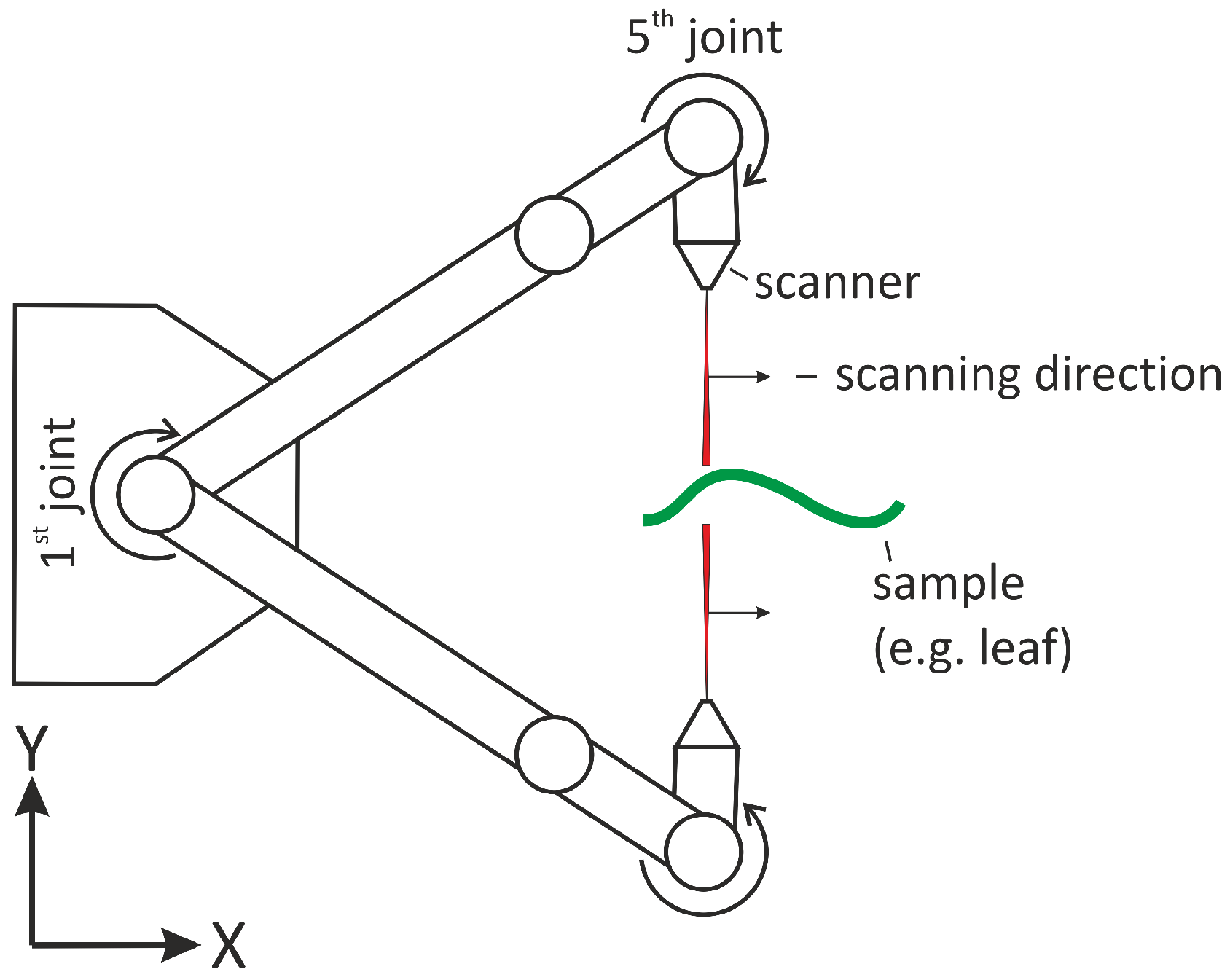
Deriving the leaf thickness requires measurements from both sides of the leaf. To minimize uncertainties caused by movements of the plant [16], the leaves were cut off the plant and fixed for the laser scanning procedure (Figure 2). This measuring setup additionally reduces the uncertainties caused by the CMA (cf. Section 2.2) because arm movements can be reduced to a minimum. As illustrated in Figure 2, only the first and the fifth joint of the CMA have to be changed a lot when scanning the upper and the bottom side of the leaf. The mechanical fixture of the leaf additionally flattens the natural leaf structure resulting in a more uniform imaging geometry of the LTS. All subsequent experiments use this setup either equipped with high precision gauges (cf. Section 3) or with crop leaves (cf. Section 4).
3. Metrological Investigation of Thickness Measurements Using Gauges
This section focuses on the metrological evaluation of thickness measurements using the appointed laser scanning system. The investigations are separated into two parts: (1) The evaluation of the CMA’s accuracy without the laser scanner using a tactile probe (only ) and (2) the evaluation of the accuracy of the combined laser scanning system ( and ). Hence, we are able to distinguish between uncertainties caused by the CMA or the laser scanner. To separate these uncertainties from uncertainties of the leaf surface (), no leaves but gauges are used providing good optical properties ().
3.1. Accuracy of the Coordinate Measuring Arm
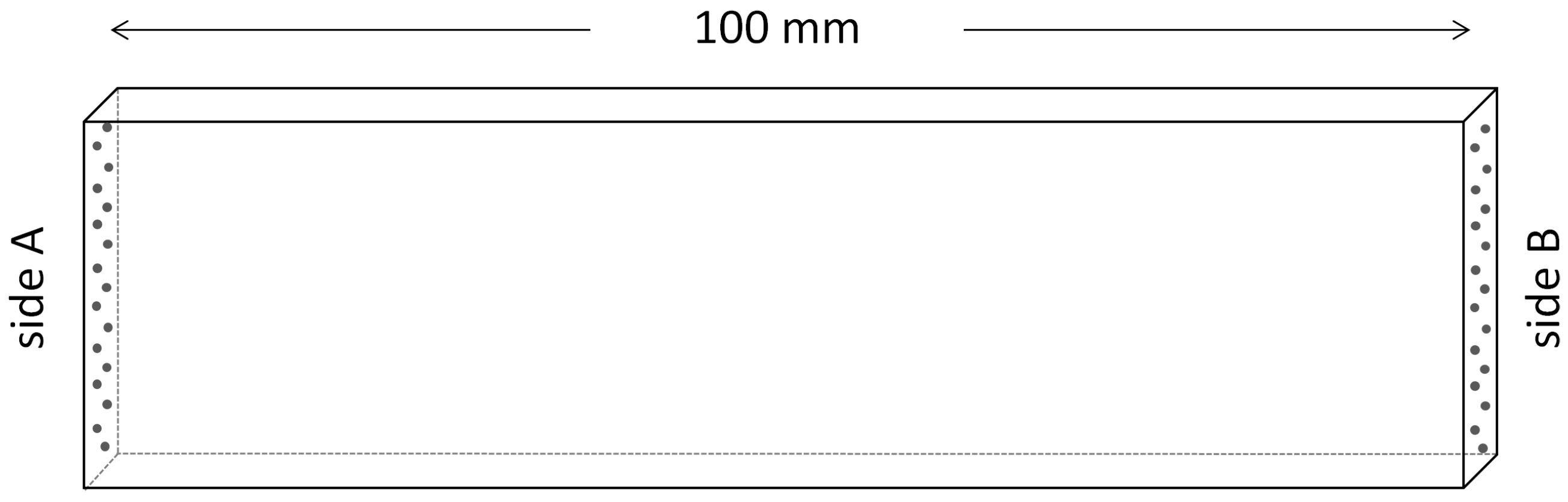
On behalf of the calibration, the kinematic parameters of the CMA can only be estimated with limited accuracy, resulting in systematic errors [22]. The errors depend on the joint configuration and will be large if the CMA is moved a lot during the measurement process. To evaluate the accuracy of the CMA, two measurement series using a high precision gauge block with a certified thickness of 100 mm ± 1.2 ×10 mm (3) were performed using a tactile probe. One measuring series comprises measurements where the joint configuration is kept nearly constant, whereas for the other series the joint configuration is changed a lot. Thus, the impact of large arm movements during the measurement can be revealed. Furthermore, the measurements were performed in a similar location to the workspace—as is the case for the leaf thickness measurements—in order to guarantee the transferability of the findings.
For the accuracy evaluation, both flat surfaces of the gauge block were measured tactile, resulting in about 100 points for each side (Figure 3). Both point clouds were approximated by the best fitting plane using an established least-squares adjustment approach [18,27]. The mean distance between the two measured surfaces, i.e., the thickness, is calculated from the distance of each point of side A to the plane of side B and vice versa. Comparing the calculated distance to the nominal length of the gauge block, the absolute accuracy of the CMA can be evaluated. The measurements were performed 10 times in order to guarantee redundancy and to reveal gross errors.
Table 1 shows the mean distance deviations to the nominal length of the gauge block and the associated standard deviation.
The results are similar to previous findings [22] and show that the deviation from the nominal length as well as the standard deviation of the measuring series increase by more than three-fold if the measurements are performed with large arm movements. Although the deviation fulfils the accuracy limits of the manufacturer of [23], it can be shown that adapting the measuring strategy can improve the accuracy of the distance measurements.
By this experiment, it can be concluded that the leaves should be placed in such a way that arm movements are reduced during the scanning process in order to minimize the uncertainties caused by the CMA.
3.2. Accuracy of the CMA Combined with the Laser Scanner
To evaluate the accuracy of thickness measurements of the combined laser scanning system, several thickness gauges with different thicknesses were measured and evaluated by comparing the measured thickness to the nominal one. The gauges were aligned in a vertical arrangement as shown in Figure 2. Consequently, the joint configuration of the CMA has to be changed minimally between the scans of the upper and bottom side of the gauge.
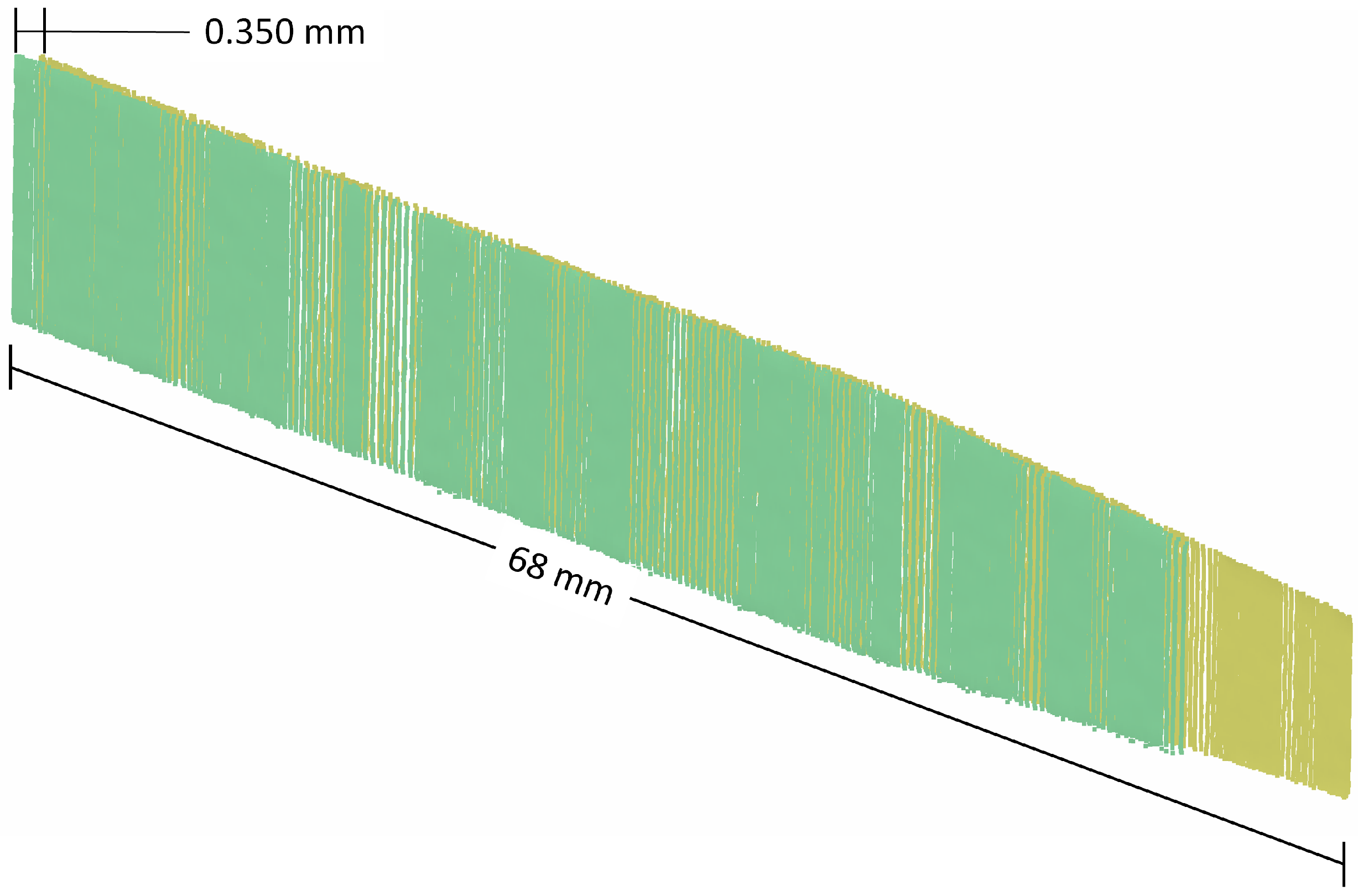
As outlined in Section 2.2, the accuracy of the LTS depends on the intensity and the shape of the laser line on the CCD-array that can be mainly controlled by exposure time. Thus, the exposure time of the LTS was adjusted automatically to the reflective properties of the gauge’s surface by applying the sensor integrated procedure. During the measurement, the scanner-surface distance and the angle of incidence were kept constant and the laser line was oriented orthogonally to the edges to minimize systematic uncertainties [18]. The results are two point clouds of the upper and bottom side of the gauges (Figure 4).
The thickness of the gauges is derived by applying the same approach as introduced in Section 3.1. Table 2 shows the target-performance comparison of three independent measurement series performed in different locations of the CMA’s workspace.
It can be found that all measurements resulted in thickness values that are systematically too large compared to the nominal ones. These systematic differences are independent of the actual thickness of the gauge. Therefore, an average deviation as well as a standard deviation can be calculated. To check whether this systematic is independent of the alignment of the gauge, measurements were repeated with a horizontal alignment of the gauges resulting in the same systematic errors.
The reason for this systematic error cannot be identified with absolute certainty and requires further research. However, further test measurements using a highly accurate spherical gauge indicate that the calibration procedure of the LTS together with the CMA may cause this systematic effect. The CMA itself can be excluded as a possible source of error, based on the measurements appointed in Section 3.1. Nevertheless, due to the fact that this systematic error appears constant in the entire workspace with a standard deviation comparable to the accuracy of the measuring system, it can be considered mathematically for each thickness measurement in the subsequent sections.
To derive the thickness with statistical certainty, the standard deviation of the two planes has to be considered. Assuming that the optical surface properties are equal for all thickness gauges, an averaged standard deviation of = 21 m for each plane can be estimated. Applying the propagation rule of variances [26] to the distance calculation, a standard deviation = 30 m is obtained. If taking into account the standard deviation of the systematic error, the standard deviation of the distance becomes = 37 m. To reach a statistical certainty of about 95%, the derived thickness should be large compared to the twice standard deviation. Consequently, using the appointed measuring system, a thickness larger than 74 m can be derived with statistical certainty.
Summarizing, it was found that the thickness measurements can be principally performed with a statistical certainty of 95% down to a thickness of ∼74 m. However, this high accuracy can only be reached for measurements performed using an optimized measuring configuration regarding the CMA on surfaces with constant and favorable optical properties for LTSs. Furthermore, a systematic error of −0.156 mm ± 0.024 mm (1) of the LTS was uncovered for thickness measurements that will be considered mathematically for each measurement in the subsequent sections.
4. Measuring Leaf Thickness of Crops
In this section, leaves of three different crops were measured and the leaf thickness is evaluated. In this case, all error sources of Equation (1) are included in the results. To obtain the highest possible accuracy, the measuring setup was designed to minimize the uncertainties of the CMA () and the LTS () based on the findings of the previous sections.
4.1. Materials and Methods
This section describes the appointed crops as well as the measuring setup and the methods used for data analysis.
Plant Material
In the experiments, the leaves of three different types of crops were used: (1) wheat (Triticum aestivum L.); (2) grapevine (Vitis vinifera L.) and (3) sugar beet (Beta vulgaris L.). The plants were grown in a greenhouse and did not show any kind of leaf damage. From each species, 10 leaves of different ages were chosen, cut off and measured directly using the measuring setup explained in the subsequent paragraph.
Measuring Setup
In order to reach the highest possible accuracy, the leaves were positioned as explained in Section 2.3 and shown in Figure 2. Analogous to the gauge measurements, the exposure time of the LTS was adapted automatically before the measurement. Furthermore, this procedure was applied for each leaf in order to compensate differences of the reflective properties caused by different ages of the leaves as investigated by Dupuis et al. [14]. In order to reveal gross errors, each of the 30 leaves was measured at least five times.
Comparative Values
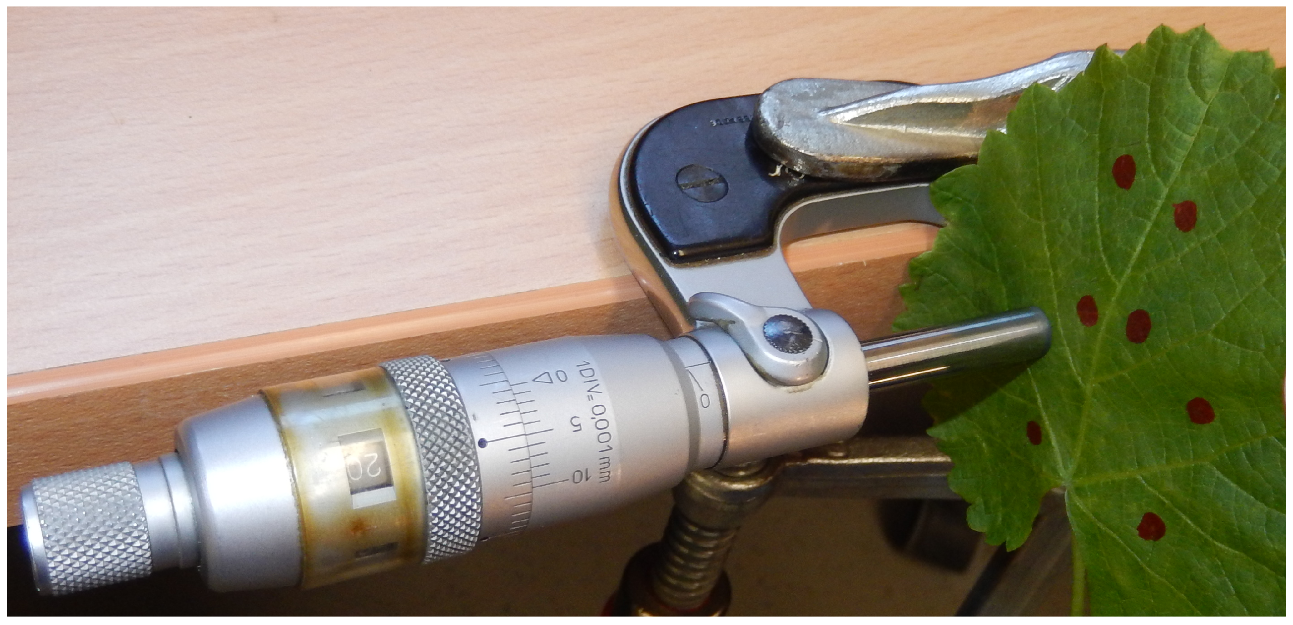
Comparative values for the leaf thickness were measured after the scanning procedure using an outside micrometer (accuracy 0.001 mm) with a torque driver and a probe diameter of 6 mm (Figure 5).
Thereby, the probe was placed on the leaf surface in such a way that no leaf veins distort the thickness measurement. Depending on the size and the shape of the leaves, 8–17 points were acquired. Due to the given measuring force, the leaf is bruised and the comparative values tend to be too small. For this reason, the invasive measurements are only comparative values instead of nominal ones. However, a more precise measurement using e.g., a microscope equipped with a coherent laser measuring system [11] is quite expensive and was not available in this study.
Calculating Leaf Thickness
Calculating the leaf thickness from two point clouds of the upper and bottom side is performed using the commercial point cloud processing software Geomagic Control (Version 2015.0.0.1904, 3D Systems, Rock Hill, SC, USA) . Principally, the leaf thickness describes the distance between the two point clouds. This is realized in Geomagic by a cloud-to-mesh distance calculation. Therefore, the point cloud of the upper side is triangulated (meshed) and the shortest orthogonal distance between each point of the bottom point cloud and the faces of the mesh is calculated. For the comparison with the invasive measurements, thickness values of the scans were averaged at the same location in a circular area with a diameter of 6 mm.
4.2. Leaf Thickness Results
This section describes the results of the leaf thickness measurements for the three types of crop.
Wheat
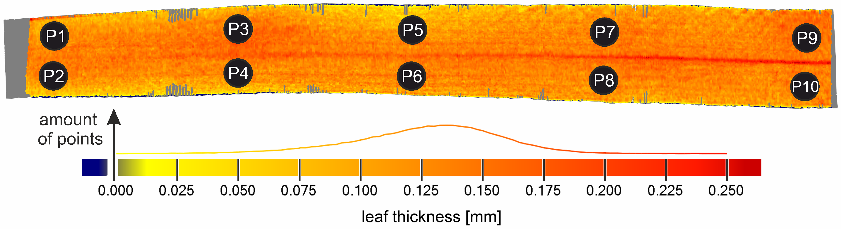
Figure 6 shows a representative point cloud of a wheat leaf colorized with the calculated thickness values. Based on the histogram and the colorization, it can be seen that the mean thickness of the leaf is in the order of 0.13 mm. Comparing the non-invasive to the invasive measured values reveals that the leaf thickness measured by the laser scanning system is systematically too small (Table 3).
Considering the whole dataset of 10 wheat leaves, this effect appears quite constant with an average deviation of 0.068 mm ± 0.015 mm (1). Although the absolute value measured is too small, an increase in the leaf thickness from the tip to the base can be found that is also visible in the tactile measurements. Consequently, it seems that the absolute thickness is not measurable but relative changes can be revealed due to the constancy of the deviation.
Grapevine
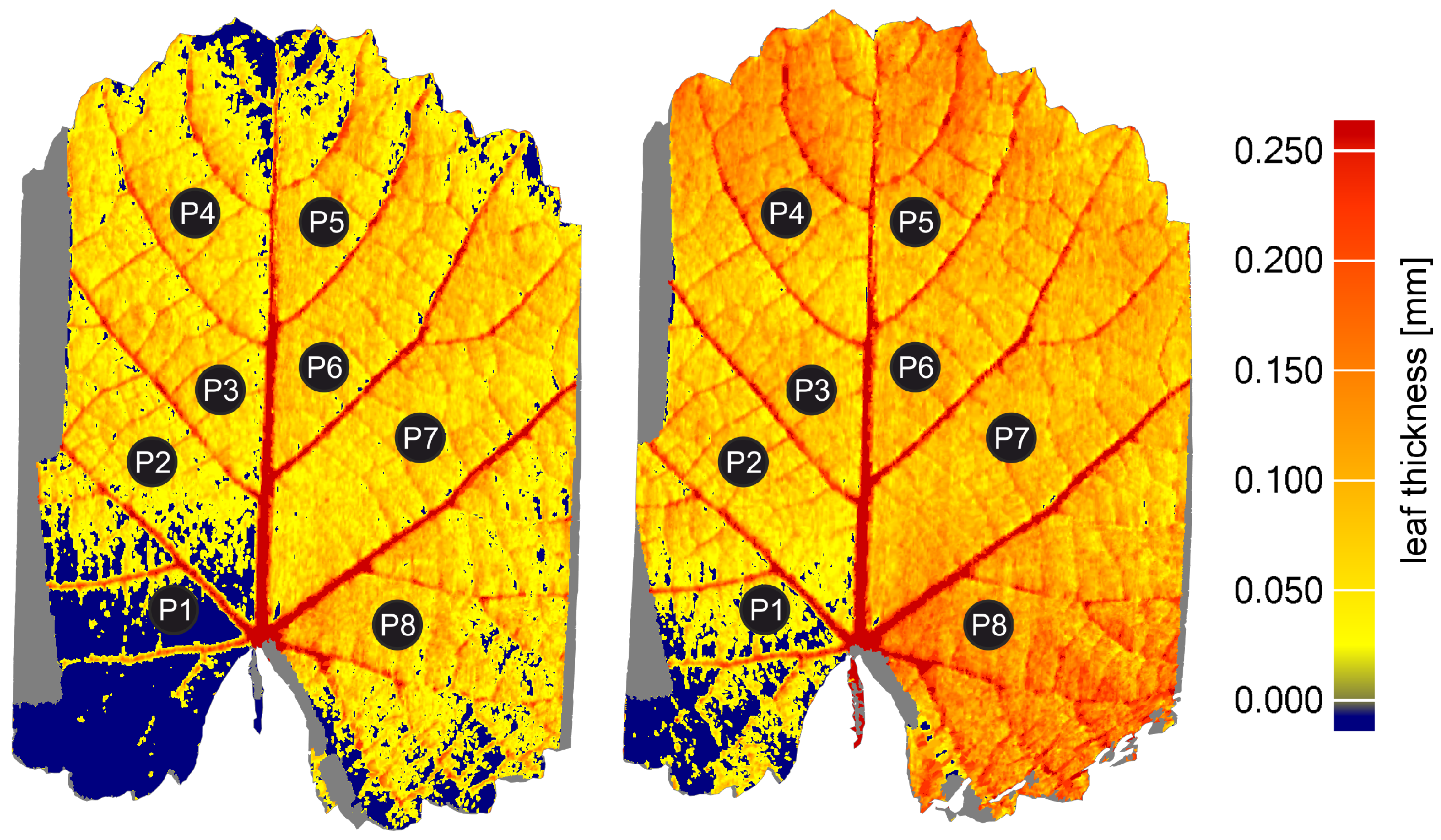
Figure 7 shows two colorized point clouds of the same grapevine leaf measured with a time lag of about 5 minutes. First, it can be found that in both scans the leaf thickness varies within the leaf area. Some regions, colorized in dark blue color, represent areas where the thickness resulted in a negative value, i.e., the point cloud of the bottom side of the leaf is above the one from the upper side. Comparing the laser scanning results to the invasive measurements, it can be found that all laser measurements are again smaller (Table 4).
Regarding the whole dataset of 10 leaves, the variations of the derived leaf thickness differences are much larger compared to the wheat leaf and can therefore not be considered constant.
Furthermore, it can be seen in Figure 7 that the color of the main leaf area, except the leaf veins, is a bit darker for the right image, i.e., the leaf is measured thicker. These effects may be attributed to small variations of the angle of incidence. Due to the cutting off, the leaf wilts and, therefore, the shape of the leaf changes during one measuring series resulting in a variation of the incidence angle. Additionally, the measuring system is hand operated, also resulting in small variations of the imaging geometry. Considering the reflective properties of the different leaf tissues [13,14], the laser is backscattered from different tissue layers for each individual scan depending on the imaging geometry.
Sugar Beet
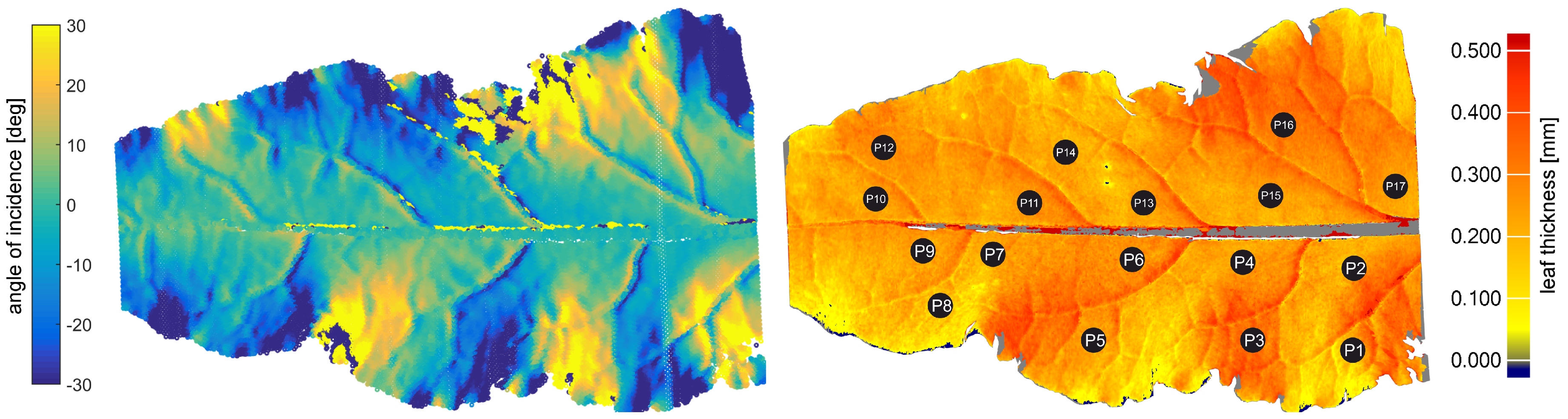
Compared to wheat and grapevine, sugar beet is the most structured and thickest crop analyzed in this study. This can be confirmed by the results in Figure 8 (right image). Similar to the grapevine, large variations of the leaf thickness can be found ranging from 0.158 mm up to 0.320 mm (Table 5).
Considering the invasive measurements, the leaf thickness differs in the range of 0.28 mm up to 0.31 mm. Consequently, it can be assumed that the variations in the laser scanning results do not represent actual differences of the leaf thickness. Compared to wheat and grapevine, sugar beet leaves are highly structured and, thus, cause changes of the imaging geometry. Although the leaves were cut off and attached almost flat, Figure 8 (left) shows that the angle of incidence of the laser plane varies within the leaf area. The angle of incidence is derived from the position and orientation of the laser plane measured by the CMA and the normal vector of the leaf surface calculated using principle component analysis.
5. Discussion
The scanning results, in comparison to the invasive measurements, have shown that the leaf thickness seems to not be accurately measurable for all appointed crops. The laser scanning approach usually resulted in smaller thickness values compared to the manual measurements and showed large variations within the leaf area. Due to the fact that the measuring setup of the CMA and the sensor properties of the LTS were optimized, the size of and is minimized and sufficient to derive thicknesses of about 74 m with statistical certainty (cf. Section 3.2). Consequently, the remaining effects can be attributed to the optical properties of the leaf surface and imaging geometry of the laser sensor, i.e., to of Equation (1).
First, the effect that the derived leaf thickness is too small in most cases can be attributed to the penetration of the laser into the leaf surface structure [13,14]. Due to the physical penetration, the laser line is displaced on the reception sensor of the LTS and the scanner-to-surface distance is measured systematically too long. This can be interpreted as a measurable penetration depth [14]. In the case of wheat leaves, this measurable penetration, with regards to the invasive measurements, seems to be relatively constant with an average of 0.068 mm ± 0.015 mm (1). This constancy can be attributed to the homogeneous imaging geometry. Because the leaves were cut off from the plant and fixed as shown in Figure 2, the angle of incidence only changes a little and the imaging geometry remains nearly constant for the whole leaf.
Considering the results of the grapevine and sugar beet leaves, the leaf thickness varies within the leaf area. In contrast to the wheat, leaves of grapevine and sugar beet are more structured, resulting in changes of the angle of incidence. Because of the optical properties of the different leaf tissues [13,14], a variation of the angle of incidence causes the signal to be originated from different leaf tissue layers. To support this hypotheses, Figure 8 shows the changes of the angle of incidence (left image) together with the variation of the leaf thickness (right image) using the example of a sugar beet leaf. It becomes obvious that the change of the leaf thickness and, therefore, the measurable penetration depth correlates with the angle of incidence of the laser plane. In areas where the angle of incidence has a large positive value (yellow), i.e., the surface is inclined in the direction of the reception optics, the majority of the imaged laser ray is reflected at the cuticle, i.e., the first surface layer. Consequently, the derived thickness value should represent the actual leaf thickness. Conversely, if the angle of incidence is negative, most of the laser ray will be reflected in the opposite direction by the cuticle and the remaining signal is originated in the mesophyll layer, resulting in a larger measurable penetration depth. Summarized, it can be concluded that the absolute accuracy of thickness measurements is low, due to the reflective properties of the leaf surface.
As explained in Section 4.1, the exposure time of the LTS is adjusted automatically to the reflective properties of the leaf surface to guarantee an optimal signal-to-noise ratio [18]. In Dupuis et al. [14], it was found that shorter exposure times cause a smaller measurable penetration depth. Consequently, one can assume that decreasing the exposure time will result in more accurate leaf thickness measurements. However, decreasing the exposure time results in a worse signal-to-noise ratio and, therefore, in higher measuring noise [18] and also a signal that is not evaluable. Thus, decreasing the exposure time to minimize the measurable penetration depth is not expedient.
Although the absolute accuracy is low, the question arises, whether it is possible to detect relative differences of leaf thickness of one species grown in contrasting environments or leaves of different genotypes. Evaluation of these relative differences is only possible if the absolute accuracy of the leaf thickness is high or if systematic uncertainties are exactly the same for all measurements. Consequently, if it were possible to measure two leaves using exactly the same measuring geometry and sensor properties and if both leaves provided exactly the same measurable penetration behavior, it would be possible to distinguish relative differences of the thickness. Regarding Figure 7 and Figure 8, this behavior cannot be guaranteed, even under laboratory conditions. Only in the case of the wheat leaf, it seems to be possible to distinguish relative differences because the measurable penetration appears quite constant. However, if there are differences in leaf thickness, one cannot clearly separate whether they are caused by different physical leaf thicknesses or by differences in the measurable penetration due to differences in the leaf structure.
All the results in this study were obtained using optimized measuring conditions regarding the CMA and the LTS. Consequently, and in Equation (1) are small. Transferring these findings to real-world measuring conditions, where the leaves are not cut off from the plant and, therefore, aligned mostly in an arbitrary way, the accuracy of the measuring system is worse, due to larger arm movements (larger ) and the effects of the imaging geometry are reinforced (larger ). Furthermore, additional impact factors () such as the movement of the plant caused by air movement or plant tropism [16] also reduce the accuracy of the resulting point clouds and the leaf thickness calculation. Hence, Equation (1) becomes
and the accuracy of the plant thickness becomes worse.
6. Conclusions
The main goal of this paper was to answer the question:
Is it possible to measure leaf thickness using an industrial high precision laser scanning system?
Although the laser scanning system is principally able to measure thicknesses of ∼74 m with statistical certainty, considering all systematic deviations and using an optimized measuring setup, the answer is "No". While the errors of the CMA can be minimized by adapting the measuring setup, the errors of the LTS are more significant. Two effects were revealed that prevent an accurate leaf thickness estimation:
- The measurable penetration depth of the laser triangulation sensor and
- the dependency of the measurable penetration on the angle of incidence.
Due to the transparency of the leaf tissues, the laser is able to penetrate the leaf surface, resulting in a systematically too long distance measurement of the LTS. Consequently, calculations of the leaf thickness resulted in smaller thickness values compared to invasive measurements using an outside micrometer. Furthermore, it was demonstrated that the measurable penetration depth varies depending on the angle of incidence. Consequently, the systematic error cannot be considered mathematically. The variability of the measurable penetration depth also prevents the derivation of relative differences of leaf thickness.
The results of this study introduce new research questions focusing on the dependency of the measurable penetration depth on the angle of incidence. If there were a unique functional between these two values, one could correct the distance measurement of the LTS by using measurements with different angles of incidence. Furthermore, it should be investigated whether the measurable penetration depends on the plant species.
The finding in Dupuis et al. [14] indicated that laser scanners with a shorter wavelength provide a smaller and, mostly, negligible measurable penetration depth. Hence, combining this kind of laser scanner with a CMA operating in the appointed measuring setup should enable the accurate derivation of leaf thickness. However, highly accurate blue laser line scanners have only emerged in the last two or three years and are rarely available for CMAs. Thus, future research on leaf thickness should focus more on using blue laser line scanners for plant phenotyping approaches.
Acknowledgments
The authors want to express their gratitude to Anne-Katrin Mahlein (Institute for Crop Science and Resource Conservation (INRES)-Phytomedicine, University of Bonn) for providing the plant material.
Author Contributions
J.D., C.H. and H.K. conceived and designed the experiments; J.D. performed the experiments; J.D. and C.H. analyzed the data; J.D. wrote the paper; All authors read and improved the final manuscript.
Conflicts of Interest
The authors declare no conflict of interest.
Abbreviations
The following abbreviations are used in this manuscript:
| CMA | coordinate measuring arm |
| CMM | coordinate measuring machine |
| LTS | laser triangulation sensor |
| CCD | charged-coupled device |
| DoF | Degree of Freedom |
| mpe | maximum permissible error |
References
- Dhondt, S.; Wuyts, N.; Inzé, D. Cell to whole-plant phenotyping: The best is yet to come. Trends Plant Sci. 2013, 18, 1360–1385. [Google Scholar] [CrossRef] [PubMed]
- Omasa, K.; Hosoi, F.; Konishi, A. 3D lidar imaging for detecting and understanding plant responses and canopy structure. J. Exp. Bot. 2007, 58, 881–898. [Google Scholar] [CrossRef] [PubMed]
- Paulus, S.; Dupuis, J.; Riedel, S.; Kuhlmann, H. Automated analysis of barley organs using 3D laser scanning: An approach for high throughput phenotyping. Sensors 2014, 14, 12670–12686. [Google Scholar] [CrossRef] [PubMed]
- Hosoi, F.; Nakabayashi, K.; Omasa, K. 3-D modeling of tomato canopies using a high-resolution portable scanning lidar for extracting structural information. Sensors 2011, 11, 2166–2174. [Google Scholar] [CrossRef] [PubMed]
- Ehlert, D.; Horn, H.J.; Adamek, R. Measuring crop biomass density by laser triangulation. Comput. Electron. Agric. 2008, 61, 117–125. [Google Scholar] [CrossRef]
- Keightley, K.E.; Bawden, G.W. 3D volumetric modeling of grapevine biomass using Tripod LiDAR. Comput. Electron. Agric. 2010, 74, 305–312. [Google Scholar] [CrossRef]
- Wagner, B.; Gärtner, H.; Ingensand, H.; Santini, S. Incorporating 2D tree-ring data in 3D laser scans of coarse-root systems. Plant Soil 2010, 334, 175–187. [Google Scholar] [CrossRef]
- Honsdorf, N.; March, T.J.; Berger, B.; Tester, M.; Pillen, K. High-throughput phenotyping to detect drought tolerance QTL in wild barley introgression lines. PLoS ONE 2014, 9, e97047. [Google Scholar] [CrossRef] [PubMed]
- Wilson, P.J.; Thompson, K.; Hodgson, J.G. Specific leaf area and dry leaf matter content as alternative predictors of plant strategies. New Phytol. 1999, 143, 155–162. [Google Scholar] [CrossRef]
- Jinwen, L.; Jingping, Y.; Dongsheng, L.; Pinpin, F.; Tiantai, G.; Changshui, G.; Wenyue, C. Chlorophyll Meter’s Estimate of Weight-based Nitrogen Concentration in Rice Leaf is Influenced by Leaf Thickness. Plant Prod. Sci. 2011, 14, 177–183. [Google Scholar] [CrossRef]
- Wuyts, N.; Palauqui, J.C.; Conejero, G.; Verdeil, J.L.; Granier, C.; Massonnet, C. High-contrast three-dimensional imaging of the Arabidopsis leaf enables the analysis of cell dimensions in the epidermis and mesophyll. Plant Methods 2010, 6, 17. [Google Scholar] [CrossRef] [PubMed]
- Wuyts, N.; Massonnet, C.; Dauzat, M.; Granier, C. Structural assessment of the impact of environmental constraints on arabidopsis thaliana leaf growth: A 3D approach. Plant Cell Environ. 2012, 35, 1631–1646. [Google Scholar] [CrossRef] [PubMed]
- Paulus, S.; Eichert, T.; Goldbach, H.E.; Kuhlmann, H. Limits of Active Laser Triangulation as an Instrument for High Precision Plant Imaging. Sensors 2014, 14, 2489–2509. [Google Scholar] [CrossRef] [PubMed]
- Dupuis, J.; Paulus, S.; Mahlein, A.K.; Kuhlmann, H.; Eichert, T. The impact of different leaf surface tissues on active 3D laser triangulation measurements. Photogramm. Fernerkund. Geoinform. 2015, 2015, 437–447. [Google Scholar] [CrossRef]
- Paulus, S.; Schumann, H.; Kuhlmann, H.; Léon, J. High-precision laser scanning system for capturing 3D plant architecture and analysing growth ofcereal plants. Biosyst. Eng. 2014, 121, 1–11. [Google Scholar] [CrossRef]
- Dupuis, J.; Holst, C.; Kuhlmann, H. Laser Scanning Based Growth Analysis of Plants as a New Challenge for Deformation Monitoring. J. Appl. Geod. 2016, 10, 37–44. [Google Scholar] [CrossRef]
- Donges, A.; Noll, R. Lasermeßtechnik. Grundlagen und Anwendungen; Hüthig Verlag: Heidelberg, Germany, 1993. [Google Scholar]
- Dupuis, J.; Kuhlmann, H. High-Precision Surface Inspection: Uncertainty Evaluation within an Accuracy Range of 15 μm with Triangulation-based Laser Line Scanners. J. Appl. Geod. 2014, 8, 109–118. [Google Scholar] [CrossRef]
- Perceptron Inc. Perceptron ScanWorks-V5 Datasheet. In Datasheet; Perceptron Inc.: Plymouth, MI, USA, 2006. [Google Scholar]
- Spong, M.W.; Hutchinson, S.; Vidyasagar, M. Robot Modeling and Control; John Wiley & Sons: New York, NY, USA, 2006; Volume 141, p. 419. [Google Scholar]
- Hartenberg, R.S.; Denavit, J. A kinematic notation for lower-pair mechanisms based on metrics. Trans. ASME J. Appl. Mech. 1955, 22, 215–221. [Google Scholar]
- Dupuis, J.; Holst, C.; Kuhlmann, H. Improving the Kinematic Calibration of a Coordinate Measuring Arm using Configuration Analysis. Precis. Eng. 2017. Available online: http://0-www-sciencedirect-com.brum.beds.ac.uk/science/article/pii/S0141635917300247 (accessed on 5 May 2017).
- Romer Inc. Romer/Cimcore Product Data Sheet, Infinite 2.0 7th Axis Portable Coordinate Measuring Machine; Romer Inc.: Wixom, MI, USA, 2008. [Google Scholar]
- Isheil, A.; Gonnet, J.P.; Joannic, D.; Fontaine, J.F. Systematic error correction of a 3D laser scanning measurement device. Opt. Lasers Eng. 2011, 49, 16–24. [Google Scholar] [CrossRef]
- Vukašinović, N.; Bračun, D.; Možina, J.; Duhovnik, J. A new method for defining the measurement-uncertainty model of CNC laser-triangulation scanner. Int. J. Adv. Manuf. Technol. 2011, 58, 1097–1104. [Google Scholar] [CrossRef]
- Mikhail, E. Observations and Least Squares; IEP-A Dun-Donnelley: New York, NY, USA, 1976. [Google Scholar]
- Holst, C.; Artz, T.; Kuhlmann, H. Biased and unbiased estimates based on laser scans of surfaces with unknown deformations. J. Appl. Geod. 2014, 8, 169–183. [Google Scholar] [CrossRef]
Figure 1.
ROMER Infinite 2.0 measuring arm combined with a Perceptron ScanWorks-V5 laser scanner.

Figure 2.
Measuring setup of leaf thickness measurements. Using this setup, only the first and the fifth joint are changed a lot when scanning the sample from both sides. All other joints are only changed slightly during the measurement process.
Figure 2.
Measuring setup of leaf thickness measurements. Using this setup, only the first and the fifth joint are changed a lot when scanning the sample from both sides. All other joints are only changed slightly during the measurement process.

Figure 3.
Sketch of the results of a tactile gauge block measurement.

Figure 4.
Representative point clouds of a thickness gauge measurement. Green points belong to the front side and yellow points to the black side of the gauge.
Figure 4.
Representative point clouds of a thickness gauge measurement. Green points belong to the front side and yellow points to the black side of the gauge.

Figure 5.
Measuring comparative values with an outside micrometer. The red areas represent the points where manual measurements were performed.
Figure 5.
Measuring comparative values with an outside micrometer. The red areas represent the points where manual measurements were performed.

Figure 6.
Leaf thickness of a wheat leaf. The meshed point cloud is colorized with the thickness values. The histogram describes the amount of points with a thickness value indicated by the colorbar.
Figure 6.
Leaf thickness of a wheat leaf. The meshed point cloud is colorized with the thickness values. The histogram describes the amount of points with a thickness value indicated by the colorbar.

Figure 7.
Two point clouds of the same grapevine leaf colorized with the calculated thickness values.
Figure 7.
Two point clouds of the same grapevine leaf colorized with the calculated thickness values.

Figure 8.
Comparison of the angle of incidence (left) and the leaf thickness (right) for a sugar beet leaf.
Figure 8.
Comparison of the angle of incidence (left) and the leaf thickness (right) for a sugar beet leaf.


Table 1.
Target-performance comparison of two measuring series of a gauge block using small and large arm movements. The values describe the average and standard deviation (std. dev.) of the 10 measuring series, resulting in more than 1500 distance calculations.
Table 1.
Target-performance comparison of two measuring series of a gauge block using small and large arm movements. The values describe the average and standard deviation (std. dev.) of the 10 measuring series, resulting in more than 1500 distance calculations.
| Small Arm Movements | Large Arm Movements | ||
|---|---|---|---|
| Nominal-Actual | std. dev. | Nominal-Actual | std. dev. |
| = 0.014 mm | = 0.003 mm | = 0.055 mm | = 0.015 mm |
Table 2.
Target-performance comparison of three independent measuring series. Units: (mm).
| Nominal Thickness | Nominal-Actual | ||
|---|---|---|---|
| Series 1 | Series 2 | Series 3 | |
| 0.050 | −0.106 | −0.167 | −0.170 |
| 0.100 | −0.126 | −0.162 | −0.169 |
| 0.150 | −0.120 | −0.180 | −0.181 |
| 0.200 | −0.133 | −0.156 | −0.175 |
| 0.250 | −0.134 | −0.151 | −0.168 |
| 0.300 | −0.131 | −0.173 | −0.170 |
| 0.350 | −0.134 | −0.154 | −0.155 |
| 0.400 | −0.125 | −0.156 | −0.165 |
| 0.450 | −0.149 | −0.193 | −0.195 |
| 0.500 | −0.158 | −0.175 | −0.165 |
| Overall Average | −0.156 | Std. Dev. | 0.024 |
Table 3.
Comparison of the invasive measured leaf thickness and the laser scanning result for the wheat leaf shown in Figure 6. Units: (mm).
Table 3.
Comparison of the invasive measured leaf thickness and the laser scanning result for the wheat leaf shown in Figure 6. Units: (mm).
| Method | Point of Comparison | |||||||||
|---|---|---|---|---|---|---|---|---|---|---|
| P1 | P2 | P3 | P4 | P5 | P6 | P7 | P8 | P9 | P10 | |
| micrometer | 0.160 | 0.160 | 0.160 | 0.170 | 0.170 | 0.180 | 0.180 | 0.190 | 0.200 | 0.200 |
| laser scanning | 0.117 | 0.100 | 0.128 | 0.113 | 0.063 | 0.111 | 0.111 | 0.123 | 0.117 | 0.133 |
| difference | 0.043 | 0.060 | 0.032 | 0.057 | 0.107 | 0.069 | 0.069 | 0.067 | 0.083 | 0.067 |
Table 4.
Comparison of the invasive measured leaf thickness and the laser scanning result for grape vine leaf shown in Figure 7 (left). Units: (mm).
Table 4.
Comparison of the invasive measured leaf thickness and the laser scanning result for grape vine leaf shown in Figure 7 (left). Units: (mm).
| Method | Point of Comparison | |||||||
|---|---|---|---|---|---|---|---|---|
| P1 | P2 | P3 | P4 | P5 | P6 | P7 | P8 | |
| micrometer | 0.170 | 0.180 | 0.180 | 0.190 | 0.170 | 0.190 | 0.200 | 0.200 |
| laser scanning | −0.063 | 0.023 | 0.034 | 0.044 | 0.046 | 0.055 | 0.072 | 0.005 |
| difference | 0.233 | 0.157 | 0.146 | 0.146 | 0.124 | 0.135 | 0.128 | 0.195 |
Table 5.
Comparison of the invasive measured leaf thickness and the laser scanning result of the sugar beet leaf shown in Figure 8 (right). Units: (mm).
Table 5.
Comparison of the invasive measured leaf thickness and the laser scanning result of the sugar beet leaf shown in Figure 8 (right). Units: (mm).
| Method | Point of Comparison | ||||||||||||||||
|---|---|---|---|---|---|---|---|---|---|---|---|---|---|---|---|---|---|
| P1 | P2 | P3 | P4 | P5 | P6 | P7 | P8 | P9 | P10 | P11 | P12 | P13 | P14 | P15 | P16 | P17 | |
| micrometer | 0.300 | 0.300 | 0.290 | 0.300 | 0.310 | 0.310 | 0.310 | 0.290 | 0.300 | 0.290 | 0.300 | 0.280 | 0.300 | 0.290 | 0.300 | 0.310 | 0.290 |
| laser scanning | 0.208 | 0.215 | 0.336 | 0.238 | 0.238 | 0.263 | 0.232 | 0.158 | 0.230 | 0.228 | 0.245 | 0.281 | 0.233 | 0.206 | 0.223 | 0.320 | 0.233 |
| difference | 0.092 | 0.085 | −0.046 | 0.062 | 0.072 | 0.047 | 0.078 | 0.132 | 0.070 | 0.062 | 0.055 | −0.001 | 0.067 | 0.084 | 0.077 | −0.010 | 0.057 |
© 2017 by the authors. Licensee MDPI, Basel, Switzerland. This article is an open access article distributed under the terms and conditions of the Creative Commons Attribution (CC BY) license (http://creativecommons.org/licenses/by/4.0/).
Share and Cite
MDPI and ACS Style
Dupuis, J.; Holst, C.; Kuhlmann, H. Measuring Leaf Thickness with 3D Close-Up Laser Scanners: Possible or Not? J. Imaging 2017, 3, 22. https://0-doi-org.brum.beds.ac.uk/10.3390/jimaging3020022
AMA Style
Dupuis J, Holst C, Kuhlmann H. Measuring Leaf Thickness with 3D Close-Up Laser Scanners: Possible or Not? Journal of Imaging. 2017; 3(2):22. https://0-doi-org.brum.beds.ac.uk/10.3390/jimaging3020022
Chicago/Turabian StyleDupuis, Jan, Christoph Holst, and Heiner Kuhlmann. 2017. "Measuring Leaf Thickness with 3D Close-Up Laser Scanners: Possible or Not?" Journal of Imaging 3, no. 2: 22. https://0-doi-org.brum.beds.ac.uk/10.3390/jimaging3020022
Note that from the first issue of 2016, this journal uses article numbers instead of page numbers. See further details here.