Segmentation and Shape Analysis of Macrophages Using Anglegram Analysis †
by
 ,
,
José Alonso Solís-Lemus
1,* ,
,
Brian Stramer
2,
Greg Slabaugh
1 and
Constantino Carlos Reyes-Aldasoro
1 1
School of Mathematics, Computer Science and Engineering, University of London, London EC1V 0HB, UK
2
Randall Division of Cell & Molecular Biophysics, King’s College London, London WC2R 2LS, UK
*
Author to whom correspondence should be addressed.
†
This paper is an extended version of our paper published in Annual Conference on Medical Image Understanding and Analysis, Edinburgh, UK, 11–13 July 2017.
J. Imaging 2018, 4(1), 2; https://0-doi-org.brum.beds.ac.uk/10.3390/jimaging4010002
Submission received: 7 November 2017
/
Revised: 15 December 2017
/
Accepted: 16 December 2017
/
Published: 21 December 2017
(This article belongs to the Special Issue Selected Papers from “MIUA 2017”)
Abstract
:Cell migration is crucial in many processes of development and maintenance of multicellular organisms and it can also be related to disease, e.g., Cancer metastasis, when cells migrate to organs different to where they originate. A precise analysis of the cell shapes in biological studies could lead to insights about migration. However, in some cases, the interaction and overlap of cells can complicate the detection and interpretation of their shapes. This paper describes an algorithm to segment and analyse the shape of macrophages in fluorescent microscopy image sequences, and compares the segmentation of overlapping cells through different algorithms. A novel 2D matrix with multiscale angle variation, called the anglegram, based on the angles between points of the boundary of an object, is used for this purpose. The anglegram is used to find junctions of cells and applied in two different applications: (i) segmentation of overlapping cells and for non-overlapping cells; (ii) detection of the “corners” or pointy edges in the shapes. The functionalities of the anglegram were tested and validated with synthetic data and on fluorescently labelled macrophages observed on embryos of Drosophila melanogaster. The information that can be extracted from the anglegram shows a good promise for shape determination and analysis, whether this involves overlapping or non-overlapping objects.
1. Introduction
The migration of cells is of great importance in many biological processes, one of them is within the immune system [1,2]. Macrophages are one of the cells within the immune system that settle in lymphoid tissues and the liver, serving as filters for trapping microbes and foreign particles [1]. Cell migration is an essential biological process that ensures homeostasis in adults, where an unbalanced migratory response results in human disease; with excessive migration causing autoimmune diseases and cancer metastasis [3]. The model organism Drosophila melanogaster can offer insights into how macrophages integrate cues to migration and other tasks [2]. It has been shown that interactions among the cells’ structures appear to anticipate the direction of migration [4]. Precise analyses of cell shapes as they evolve through time, as well as the correct identification of interacting cells that overlap could provide information for specific cells in biological studies; where sharp corners suggest an active migrating cell and rounded corners inactivity [4]. Thus, accurate cell segmentation could provide information for specific cells for biological studies.
Segmentation of cells in fluorescence microscopy is a widely studied area [5,6], with many approaches ranging from thresholding techniques [7], to active surfaces [8] and active contours [9]. In recent years, techniques such as adaptive active physical models [10] and multilevel sets [11] have been used to address the problem of cells that overlap in cervical cancer images. Other techniques including self-organising maps (SOM) have also been used for biomedical image segmentation [12]. When the cells overlap, the segmentation problem in a single frame becomes more complicated as the imaging does not produce reliable borders for the cells, even through human inspection. For example, thresholding [13] and curve evolution methods [9,14] can only detect clusters of cells. In works like that of Plissiti and Nikou [10] and Lu et al. [11], the data allow a priori shape models based on simple shapes, whereas the data presented in this work needs a more complex analysis that focuses on shape features and its junctions. On the boundaries of objects, junctions are commonly acquired by looking for extrema in the curvature of the image gradient [15,16]. Since an assumption for a simple shape cannot be made for the fluorescently labelled macrophages presented in this work, a thorough shape analysis for both overlapping and non-overlapping cells should be made. This paper describes a novel approach to find junctions of boundaries of single and overlapping objects, and provide cases for its application. Two classes of junctions are studied: (i) bends in boundaries of overlapping objects, whose intersections would correspond to the junctions acquired; and (ii) corners, which correspond to the pointy edges in single objects. The corners detected, and the methodology to do so would provide a tool for the analysis of shape. On the other hand, the bends would be used as the basis for completing a segmentation of the overlapping cells, four methods are presented of which three use the information from the bends detected.
A preliminary version of this work was presented at the 21st Medical Image Understanding and Analysis (MIUA) [17]. The algorithms have been extended and this work now describes the following topics, which were not included previously: (i) distinction between two different types of junctions, as they apply to overlapping and non-overlapping objects; (ii) analysis of shapes in single (non-overlapping) objects, which introduces a notion of pointiness in a determined shape, applied to cell shapes; (iii) deeper statistical analysis of previous results; (iv) intermediate steps’ results presented to outline the entire procedure: detection of objects, of junctions, and into applications (segmentation of clumps); and (v) a thorough explanation of the anglegram matrix and its construction.
2. Materials and Methods
2.1. Macrophages Embryos
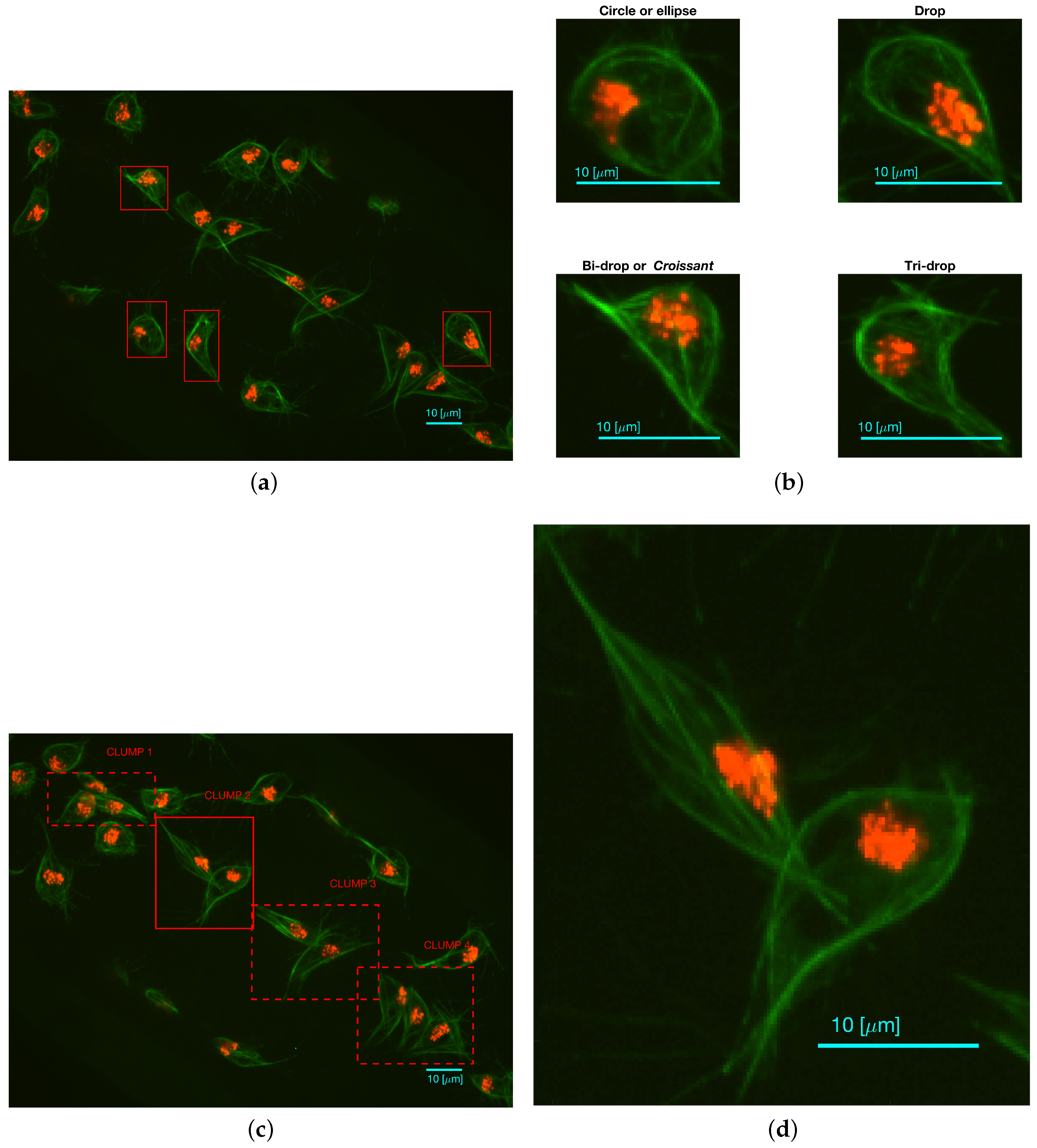
Fluorescently labelled macrophages were observed in embryos of the model organism Drosophila melanogaster. The nuclei were labelled with GFP-Moesin, which appeared red, whilst the microtubules were labelled with a green microtubule probe (Clip-GFP) [4]. RGB images of dimensions and 541 time frames were acquired. The images have two layers of fluorescence. Figure 1a presents one representative time frame where four basic shapes can be recognised: circles or ellipses, drops, which have one sharp edge like a water drop, bi-drops or croissants, which have two edges and tri-drops which is similar to a drop but with three pointy edges. A close view of the shapes can be seen in Figure 1b. The data does not show instances of cells with more pointy edges. To illustrate the overlapping of cells (clumps) found in the data, Figure 1c shows one representative time frame where clumps are present. The green channel illustrates overlap that makes an accurate segmentation of the cells complicated. Figure 1d shows the detail of one of the clumps.
Ground Truth of Macrophages Data
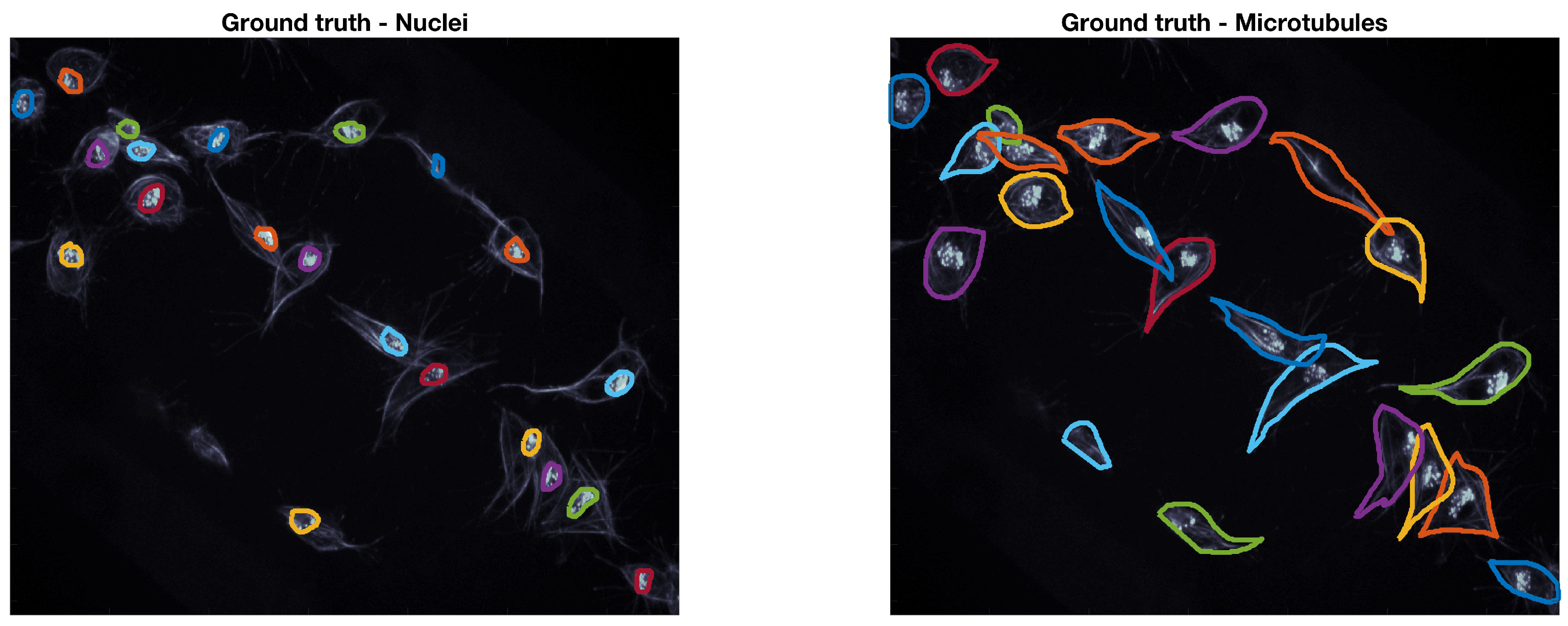
The ground truth (GT) used to accommodate this data was built through a Matlab® software developed by the authors. The GT software, which is based on Matlab®’s imfreehand function, allows the user to manually label images of cells, accounting for the overlap. The user labels all cells of interest in both red and green channels of the data. In this work, a subset of ten frames from the original 541 images were manually segmented by the authors, the frames selected present examples of overlapping that can be recognised and studied, namely the four CLUMPS depicted in Figure 1a. An example of both manually segmented channels can be seen in Figure 2.
2.2. Synthetic Data
In order to assess the limitations of the junction detection methodology, two types of synthetic images were generated for the two types of junctions described in this work: bends and corners. For the detection of bends, one hundred and forty two images of pairs of synthetic overlapping ellipses were generated. Such images covered the varying angles and separation distances covering the span of possible study cases. For the detection of corners, the images representing the basic shapes previously described were generated through a number of moving control points.
2.2.1. Synthetic Data of Overlapping Ellipses
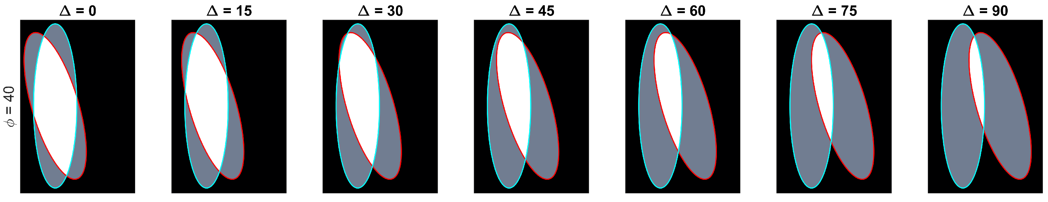
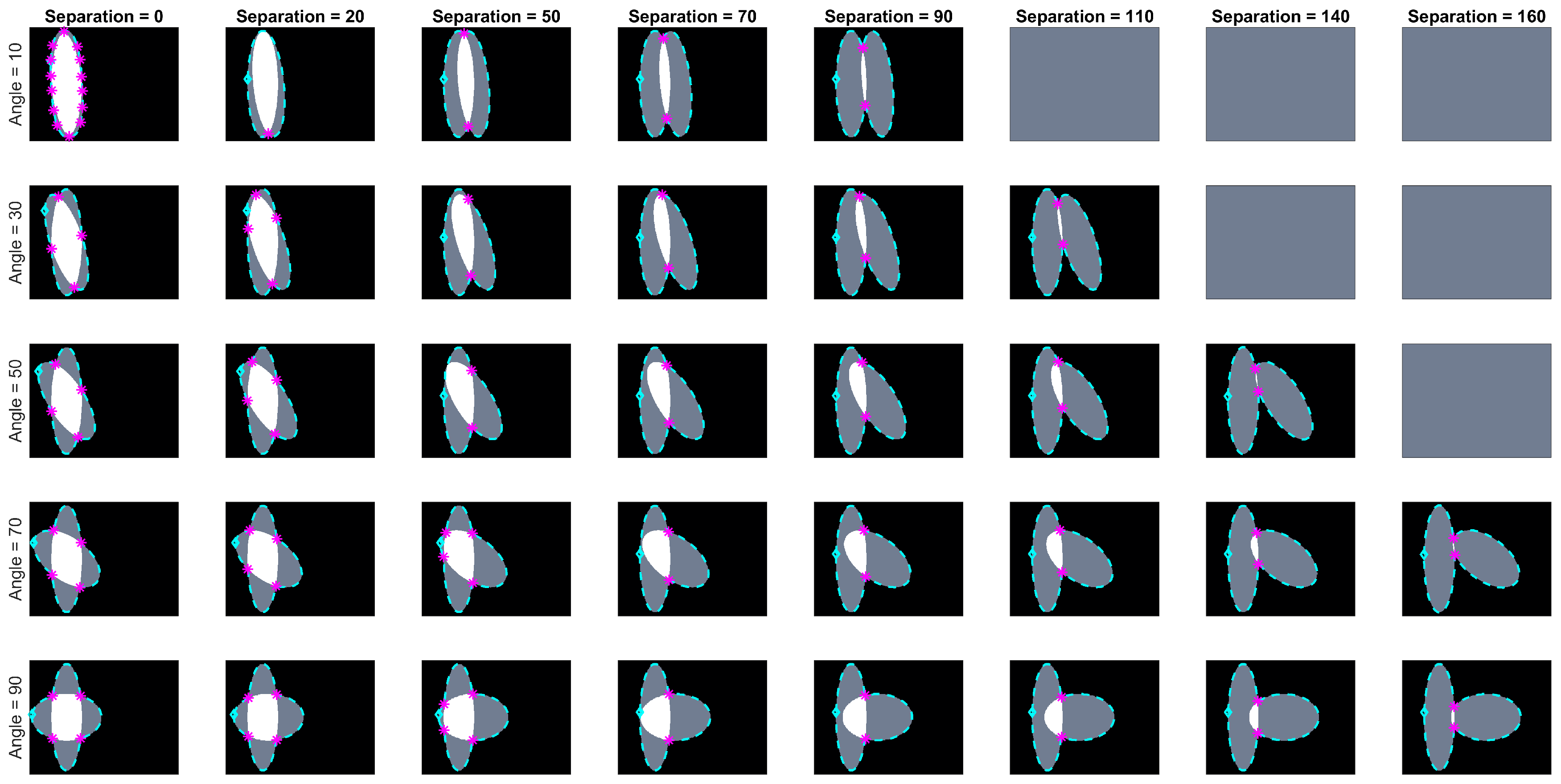
Let be the ellipse defined by the equation , which is rotated with respect to the x-axis by degrees and whose centre is located on position . The paired ellipses constructed in this work differ both in angle and position with three conventions taken into consideration: (i) presetting the values of the axes ; (ii) defining a central ellipse , common to all pairs; and (iii) the difference in position would only be made by moving the ellipses in the x-axis. Thus, the paired ellipses can be defined in terms of the differences to , namely the angle and distance from the centre . A set of paired ellipses was generated in Matlab® to test the method at different values of ranging from 0 to 90 degrees and from 0 to 160 pixels with increments of 10. Images of size were generated with and axes that contained an overlapping of and . Disregarding the images where there was no overlap present in the generated ellipses, a total of 142 images was generated. Figure 3 contains a subset of the ellipses tested. Cases where there was no overlap were ignored from the analysis.
In this work, a clump will be understood as a cluster of two or more overlapped objects. A clump was detected when two or more nuclei on the red channel were detected within a single region on the green channel.
2.2.2. Object Detection: Single Objects and Clumps
Segmentation of the green channel was performed by low-pass filtering with a Gaussian filter, following with a hysteresis thresholding technique [7]. A morphological opening with a disk structural element () was performed to smooth the edges and remove noise. Segmentation of the red channel followed the same methodology. Then, the number of nuclei per region was counted to determine the presence of clumps.
2.2.3. Basic Shapes Synthetic Data
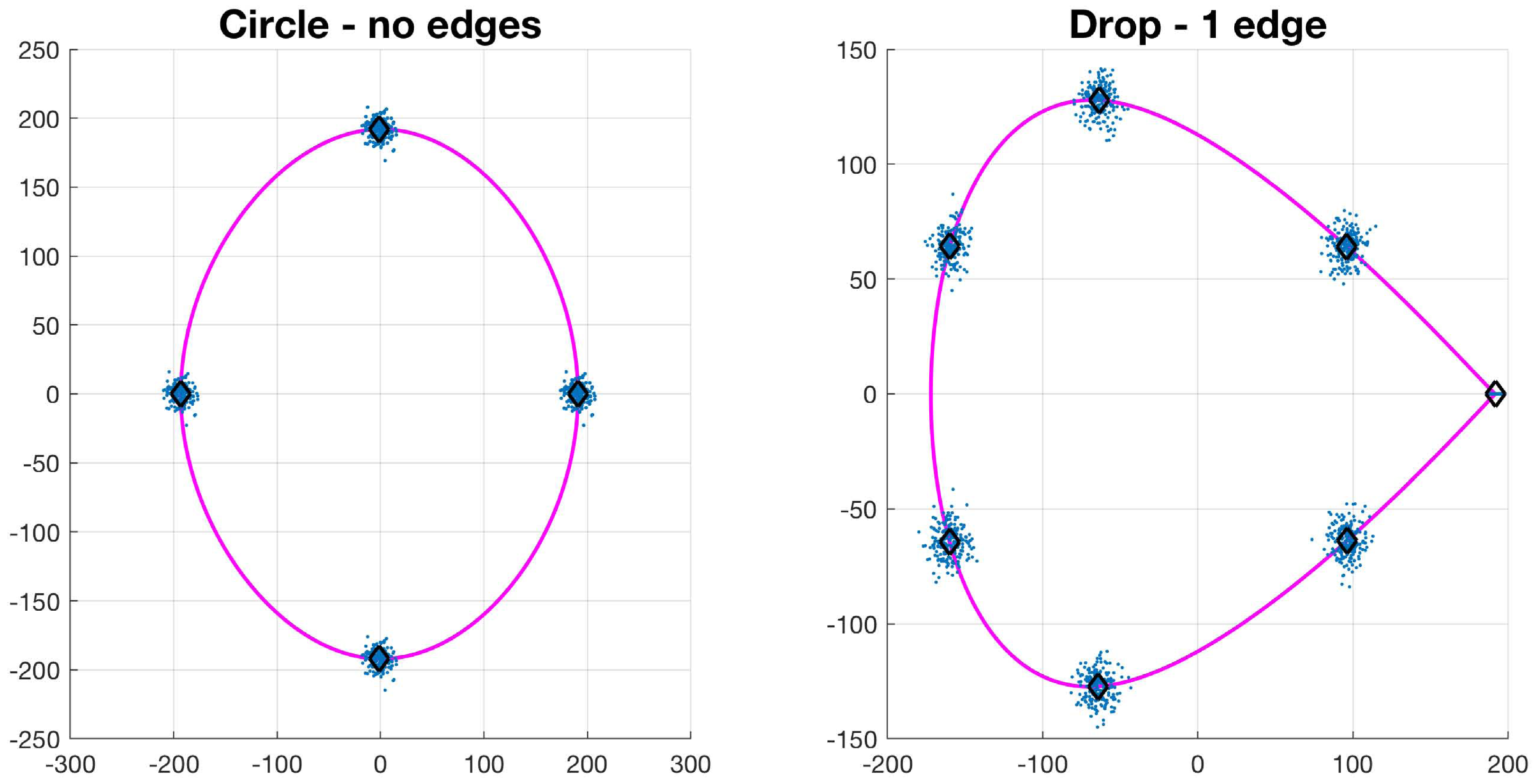
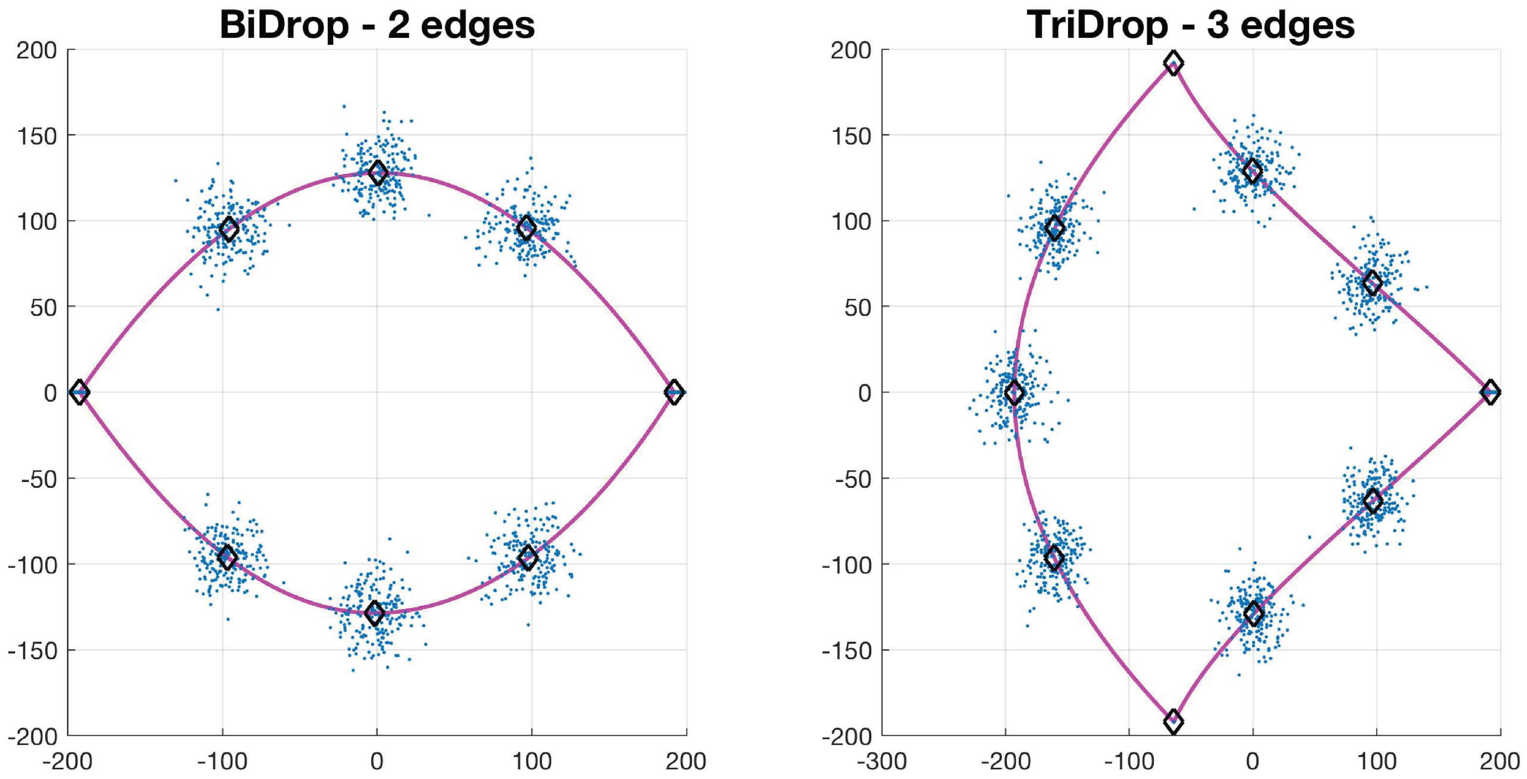
Let , be a collection of N control points of a basic shape such that . The value of N depends on the type of basic shape: circle has 4, drop has 7, bi-drop has 8 and tridrop has 10. To model the variations in the cells’ shapes, within their basic categories, the control points are distributed Normal. It is easy to see that each shape has a specific number of corners that classify them, i.e., the drop has one pointy edge or corner, while bidrop and tridrop have two and three, respectively. The control points are joined with splines that then produce the boundary of the shape, , which then models that of a segmented cell (Figure 4). In this work, the shapes explored in detail were drop, bidrop and tridrop, where only the corners were moved to modify the pointiness of each shape and the rest of the control points were kept stationary. The pointiness value of each shape was chosen empirically between a rounded version of each shape and a pointy one. These values were allocated in a scale that ranges from 0 to 1.
2.3. Junction Detection through Angle Variations
Let define the boundary of a clump or a single object, then for each of the ordered points , the inner angle of the point is defined as follows,
Definition 1 (Inner angle of a point).
The inner angle of a point in the boundary is the angle adjacent to the point, and measured from the jth previous point to the following jth position . The angle is then depicted as .
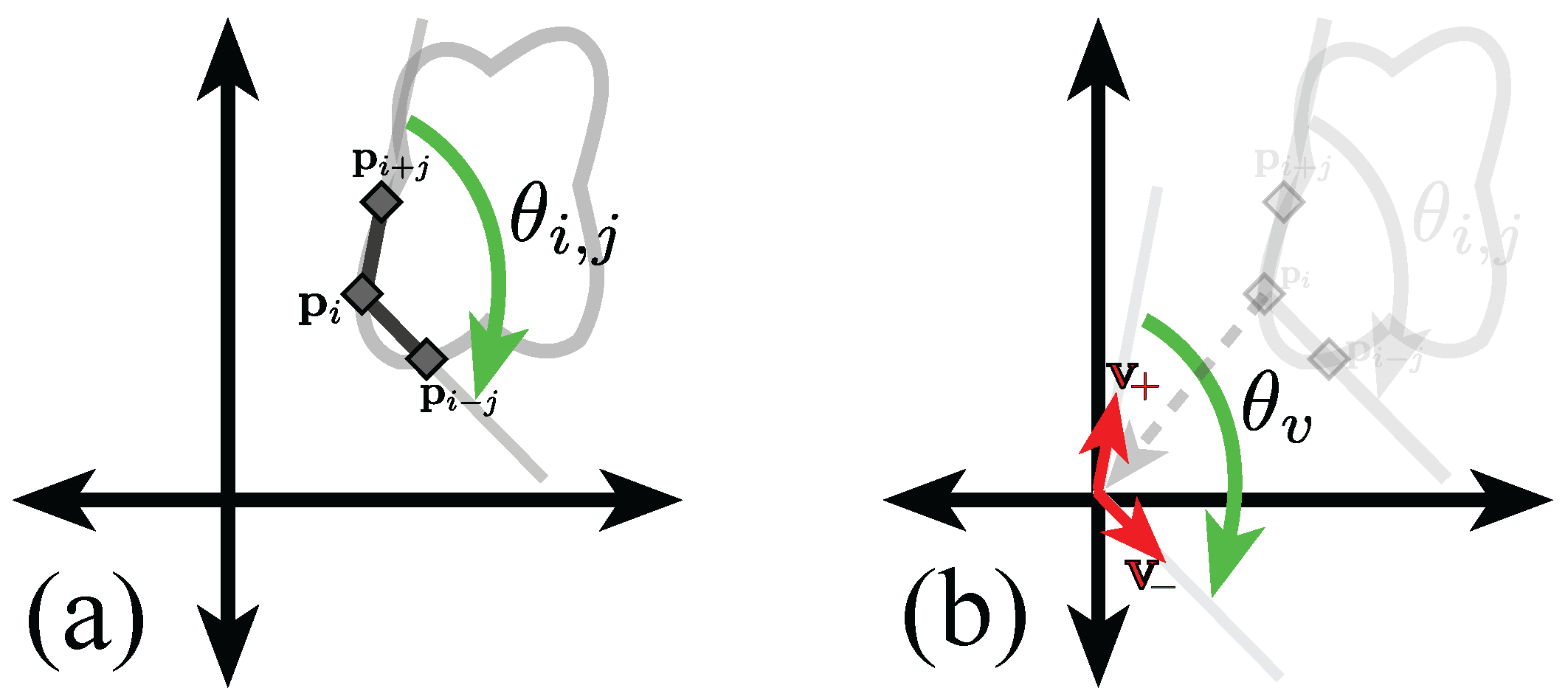
For clarification purposes, a brief mathematical derivation of the inner angle of point , with separation j, is presented, with an explanatory diagram shown in Figure 5.
Let , the jth previous and following positions in the boundary are , respectively. Let the vectors be defined as , and . The angle, , adjacent to the origin and measured from to will be equal to the inner angle of the ith point, . Finding the angle is done through Equation (1).
Given the previous definition, a more accurate description of the types of junctions is defined in this work as follows,
Definition 2 (Bend and corner junctions).
A bend is a junction in which the inner point angle for most separation distances is greater than 180 degrees. Conversely, a corner is a junction in which most of its inner point angles are acute, i.e, less than 180 degrees.
Figure 6 and Figure 7 show examples of the calculation of an inner angle for a given point in a clump boundary, the calculation is the same for single objects. For simplicity, the detection of junctions will be described extensively for the case of bends, as in [17]. Then, the modifications to detect corners will be outlined. By visual inspection, it can be noticed that the inner angle of a junction would be greater than 180 degrees for a number of separations j. This number of separations will be referred to as the depth of the junction. Thus, the method consists of computing the inner angle at every point , and on every separation j.
Definition 3 (Anglegram matrix).
The anglegram matrix is defined as the values of the inner angles of each point i and per separation j, that is .
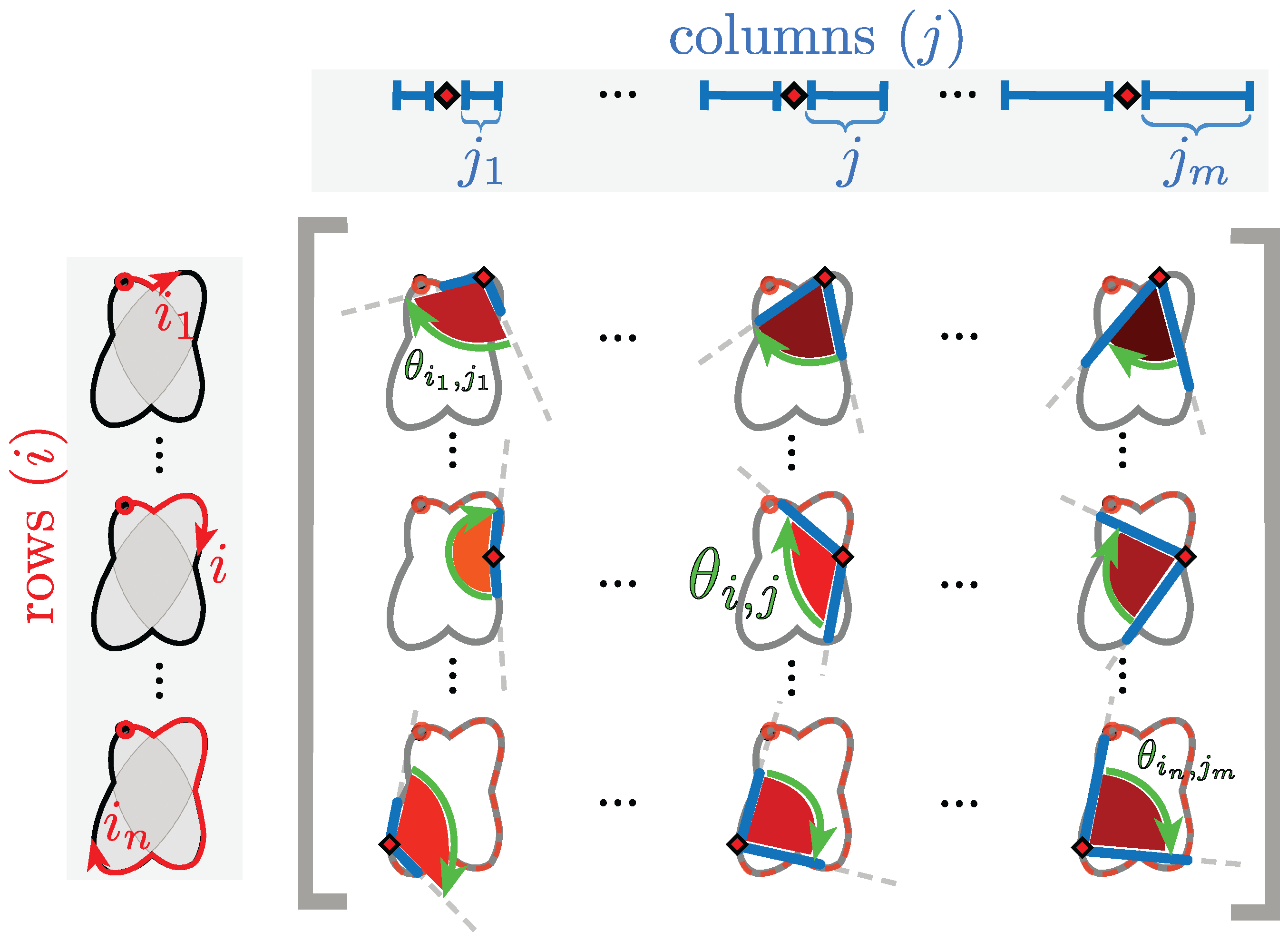
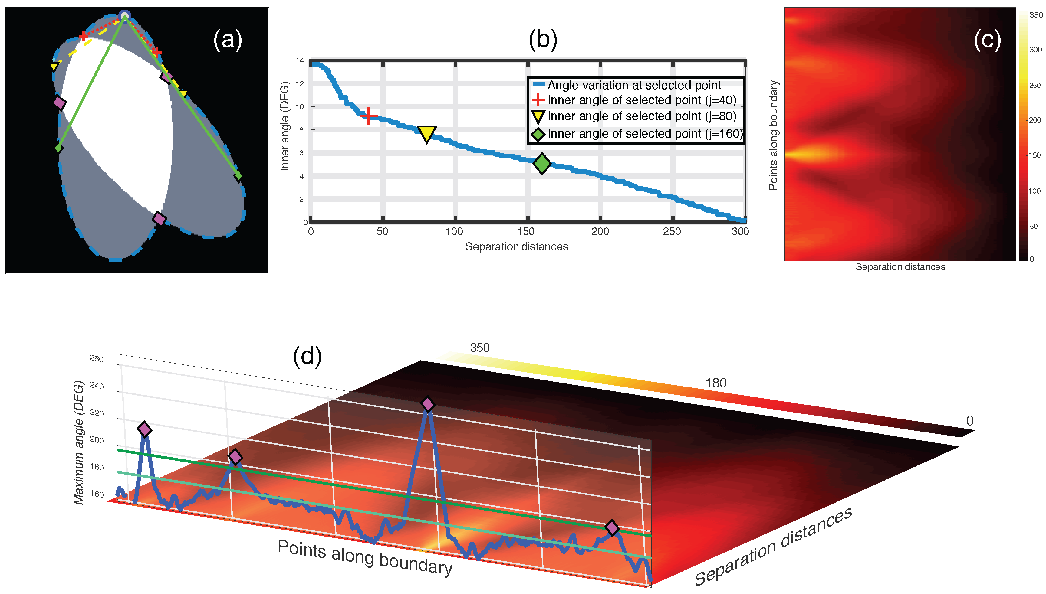
In the anglegram, the columns represent the separation distance and the rows represent each point in the boundary. This process is depicted in the diagram of Figure 6. Furthermore, Figure 7 contains an example of this construction in a synthetic case, where (b) shows a single row of the anglegram, whose values correspond to a single point (blue ○) and three instances of the inner point calculation at different separations (red+, yellow ∇ and green ⋄).
Criteria to Detect Junctions from the Anglegram
The local maxima on a projection over the horizontal dimension of the anglegram is related to the position of the junctions of the boundary and the depth of the junction. Each row, , corresponds to the inner angles of point , therefore taking a summary of the rows would yield a measurement of the general inner angles of each point. For this work, the maximum intensity projection , Figure 7d, was compared with the mean, median and area under the curve, but the maximum provided the best results (data not shown). To account for quantisation errors in the boundaries extracted from the clumps, an averaging filter of size was applied to the anglegram matrix, , before the calculation of . The local maxima of the 1D projection were found by using the function findpeaks from Matlab®, which identifies local maxima of the input vector by choosing points of which its two neighbours have a lower value. Due to quantisation noise in , the parameters MinPeakDistance and MinPeakHeight were set to empirically consistent values. First, MinPeakDistance, which restricts the function to find local maxima with a minimum separation, was set to 25. Furthermore, the parameter MinPeakHeight was set to .
To detect corners, two alterations were implemented: (i) resizing the anglegram to have 64 rows to reduce noise; and (ii) taking the mIP of the first half columns, as the final columns are lower by the definition of the inner point angle measurements. An extra condition was added to avoid over-detecting corners in circles: when detecting over four corners with a mean value greater than 120 degrees, the corners detected are discarded.
2.4. Segmentation of Overlapping Regions
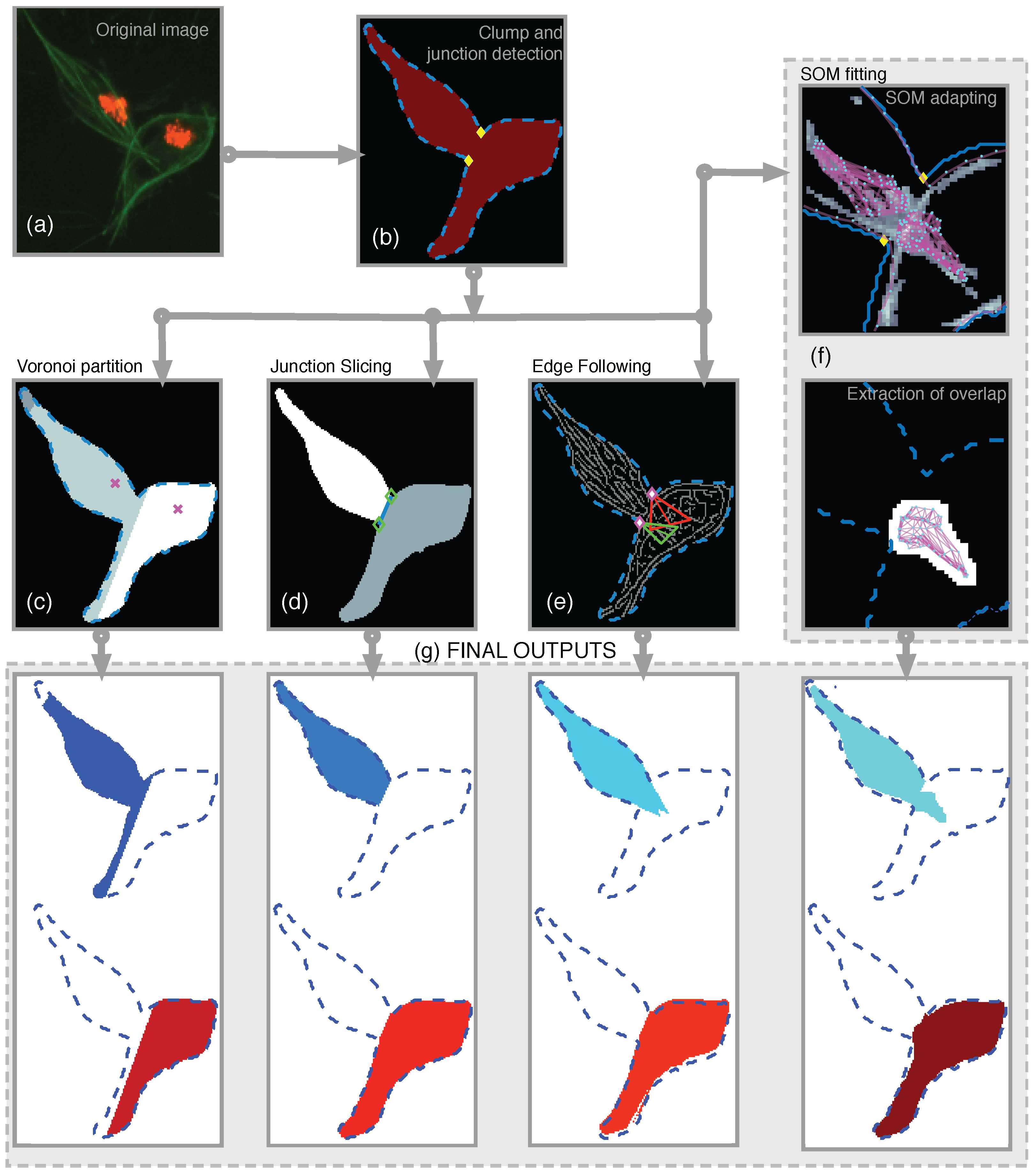
This section describes the comparison of methodologies to segment clumps into overlapping cells. Initially, as a benchmark, a simple partition of the clump based on Voronoi partitioning [18] was developed. Then, the three methods, which incorporate the information from the junctions into a segmentation output were used. The methods differed in the way the junctions’ information was incorporated into a complete segmentation. Junction Slicing (JS) and Edge Following (EF) involved the explicit use of the junctions’ position, while the proposed self-organising map (SOM) fitting involved the information of junctions into creating a custom SOM that adapts to the overlapping section of the data. In this work, only the cases where two junctions were found were examined in detail. A diagram showing all methods presented and the data flow is presented in Figure 8.
2.4.1. Voronoi Partition
This method was included as a lower-bound benchmark for comparisons against with the proposed methods. It consists of a naïve approach to the problem that does not include any information from the green channel. The image area was partitioned, using Voronoi tessellations [18]. The partition of the space was based on the centroids of the detected nuclei from the image’s red channel. The clumps detected on the green channel were divided based on the Voronoi partition.
2.4.2. Junction Slicing (JS)
This method partitioned the clump with the line that joined two junctions. For each junction detected, each of the two adjacent segments of the boundary of the clump would correspond to one of the different objects within the clump. Since the points in the boundary are ordered, starting at one point and moving alongside in a clockwise manner, then the segment that appeared before a detected junction would correspond to one cell, whereas the segment that appeared after the junction would correspond to the other cell. For cases where only two junctions were found, the problem of selecting which pair of junctions will be joined becomes trivial. However, considering a case like the one presented on Figure 7a, where four junctions would appear, different combinations of the boundary segments could yield different candidates of segments.
2.4.3. Edge Following (EF)
In order to obtain the edge information, the Canny [19] algorithm was used on the green channel of the image. The algorithm consists of finding the local maxima of the image gradient. In this work, the parameter of the standard deviation was set to . The trend of the two adjacent segments leading to the junction was defined by approximating the tangent line of the boundary at the junction point. The definition of the tangent line was taking an average slope of the secant lines leading up to the detected junction. The tangent line was extended, and a region of interest (ROI) was defined by a triangle where the approximated tangent line goes along the vertex and the adjacent angle corresponds to 20 degrees to each side of the tangent line (Figure 8). The ROI defined for each of the adjacent line segments was then intersected with the edge information of the image, resulting in a set of binary line segments, which were labelled. Labelling of the binary line segments allowed for individual analysis of each line. Each line detected was analysed in terms of its orientation and size, preserving the one that has the most similar orientation to the extended line segment. Binary line segments with a change in direction were split by removing the strongest corners, detected through the corner detection algorithm by Harris and Stephens [15]. The lines found by both ROIs on each junction were then used as new coordinates to add to the boundary of the corresponding cell.
2.4.4. Self-organising Maps (SOM) Fitting
This work proposes an alternative implementation of the self-organising maps [20] that adapts itself to the overlapped area. For this SOM, a custom network was defined, as well as the input data and additional rules to the definition of the step-size parameter, . Let a Network , where are nodes assigned to positions in the plane and are some edges linking the some of the nodes in . Each node has an identifier, position, and a speed parameter, related to the movement of each node. The input data was determined by the positions and normalised intensity values of the image, i.e., . Values in that were selected by an Otsu’s threshold [13], and were located within a bounding box that contains the junctions. Given an input, the algorithm proposed by Kohonen [20] follows two basic steps: identifying the closest node in the network to the input, shown in Equation (2), and update the positions of the nodes inside a neighbourhood, determined by a distance to the winner node , (3),
where refers to the distance from node i to node j in the shortest path determined by the edges . In this work, the parameter was determined the intensity level of the image, I, and the speed parameter of the node. The proposed formula for the parameter is shown in Equation (4),
where is , or 1, depending on where the node resides in the topology. The network was defined by taking a subset of the boundary points in in a ring topology, and then adding two networks in a grid topology to each side of the line joining two junctions. The three networks are independent from each other. Thus, , if was located in the boundary of the clump, and , if it was one of the grid networks. The assumption is that the network taken from would be closer to the actual cell, and therefore it should not move abruptly, whereas the networks inside the clump will adjust and adapt to the shape of the overlapping area between the cells. In order to finalise the network final state into a segmentation, the external network was taken as a new clump and it was partitioned by the same line used in the junction slicing (JS) method. Finally, the area formed by the inner network that adapted to the overlapping section of the cell was dilated with a square element and then attached to both partitions of the new clump. Figure 8f displays the main steps of the SOM fitting method described.
3. Results
Experiments were performed on synthetic data of both overlapping and single objects, allowing the determination of limits of the junction detection methodologies presented in this work. The methodologies include the use of the anglegram matrix [17], explained in Section 2.3. The junction detection, of both bends and corners, is presented for the synthetic images. Then, for the macrophages data, the junction detection is presented and compared against the Harris junction detector [15], which was applied on the binary images using the detectHarrisFeatures in Matlab®. Finally, the results of the proposed segmentation techniques of the overlapping cells (Section 2.4) are shown, starting with the detection of objects explains in Section 2.2.2.
3.1. Bend Detection in Overlapping Objects
Images of overlapping ellipses with varying ranges of angles and separations were analysed. Based on the corresponding value in the maximum intensity projection (MIP) of the anglegram matrix, given the methodology explained in Section 2.3, the junctions that were correctly detected on the synthetic data had a range of angles [–] degrees; whilst the missed junctions had a range of [162–] degrees. This indicates that very wide angles, close to a straight line are easy to miss. The overlap region of [188–192] degrees deserves a further investigation outside the scope of this paper. A correct detection would place the junction within 5 pixels of the known intersection of the boundaries. A subset of the tested synthetic ellipses with their detected junctions (bends) is depicted in Figure 9.
3.2. Corner Detection in Single Objects
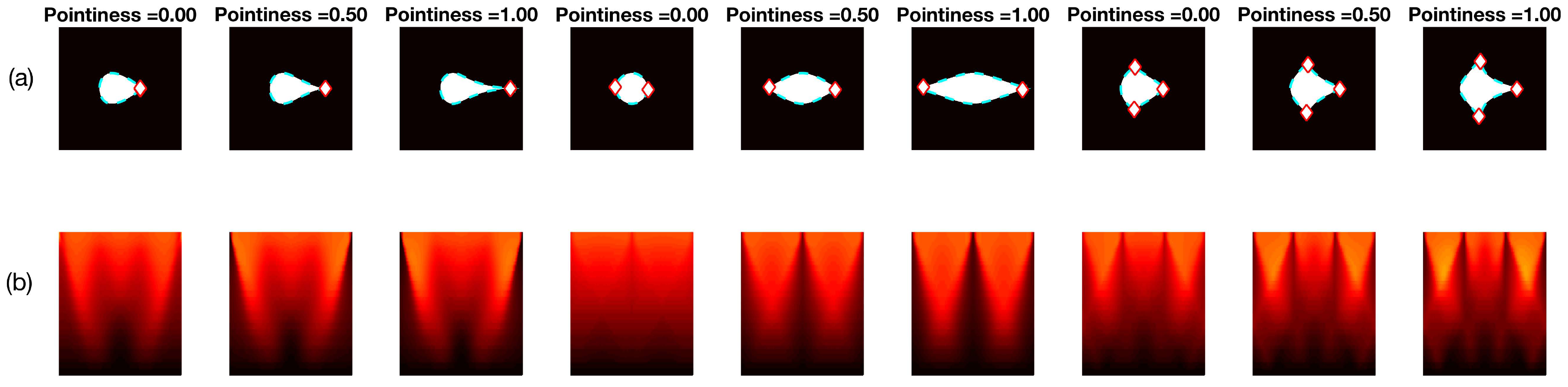
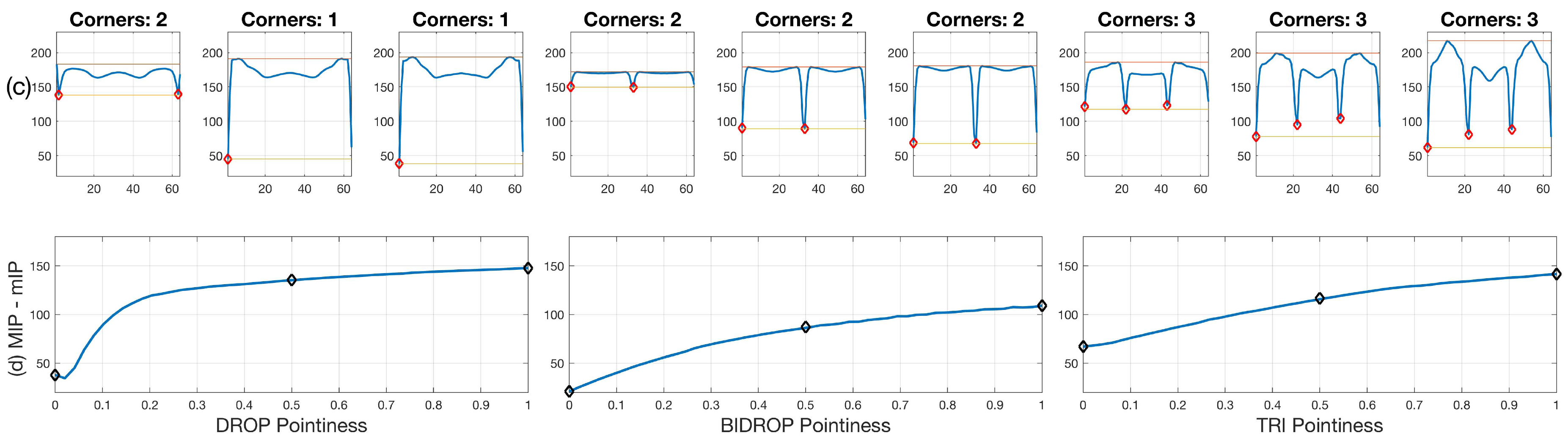
Two different sets of synthetic images were analysed, based on the descriptions in Section 2.2.3. The first experiment, involving Figure 10 shows the different sharpness level (pointiness) of the basic shapes, respectively: drop, bi-drop (or croissant) and tridrop. Each figure presents the relationship of the shape and pointiness it has with the anglegram. For each basic shape, three instances of the shape with varying pointiness values are shown (a). The boundaries are depicted in a dotted line (cyan - -) and the corners in red (⋄). The anglegram matrix for the displayed shape is presented in (b). The values of the anglegram can range from 0 to 360 degrees. In (c), the minimum intensity projection (mIP) of the anglegram is shown, where the horizontal axis represents the points along the boundary and the vertical axis represents the angle in degrees. Maximum and minimum values of the mIP are shown as solid lines. The positions where the corners were detected are depicted in red (⋄). The minimum and maximum values of the mIP are displayed as horizontal lines for visualisation purposes. Finally, in (d), the difference between the maximum and minimum values of the mIP for 50 different values of pointiness is shown. This difference seems to be growing proportionally to the pointiness level. The values of the displayed shapes in the top row are highlighted (⋄).
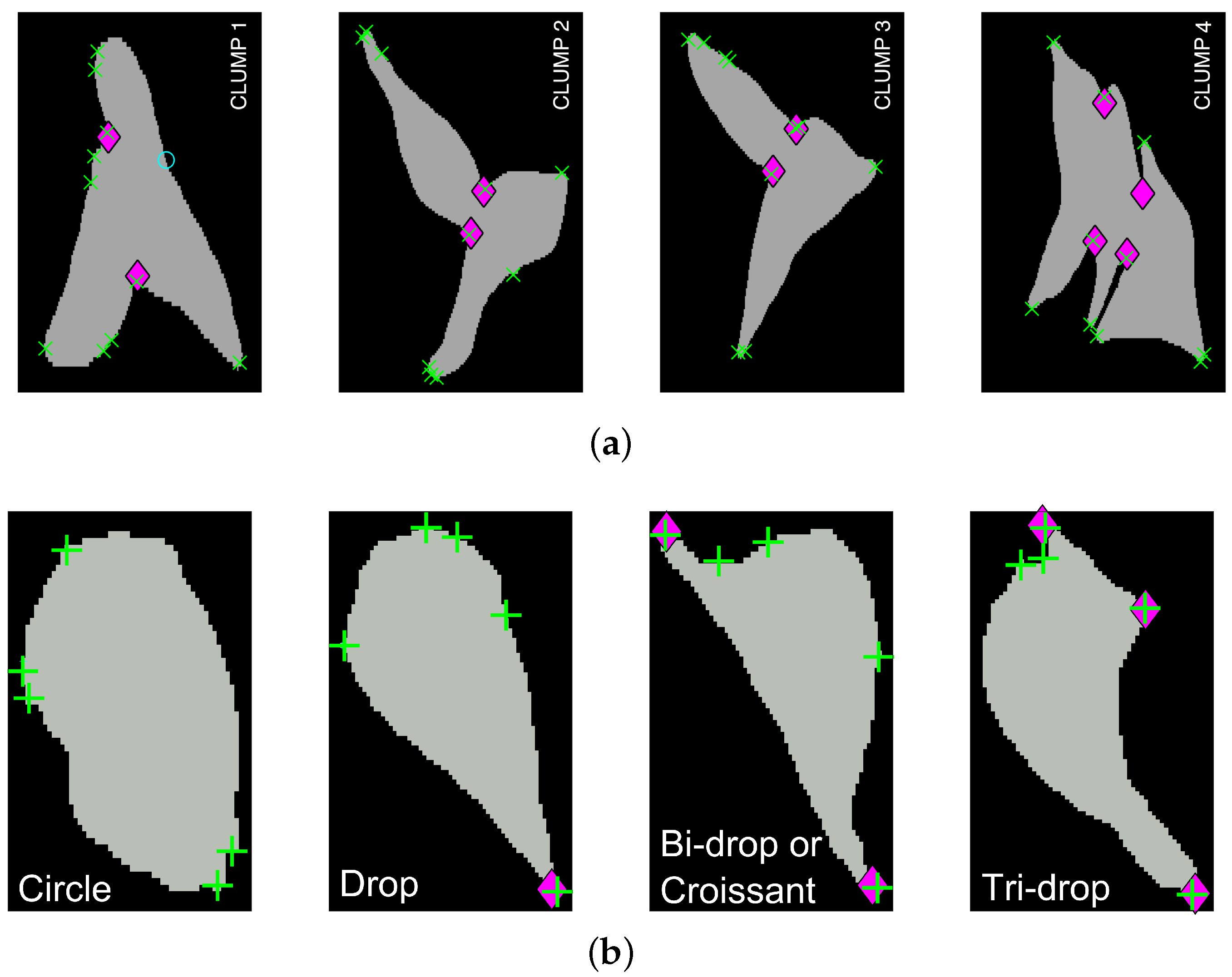
For four overlapping clumps, which can be seen in Figure 1a, junctions (bends) detected by the anglegram algorithm were compared qualitatively against the Harris corner detector [15], as can be seen on Figure 11a. Conversely, a similar comparison for the corner detection method of the four basic shapes is shown in Figure 11b.
Detection of Objects and Segmentation of Clumps
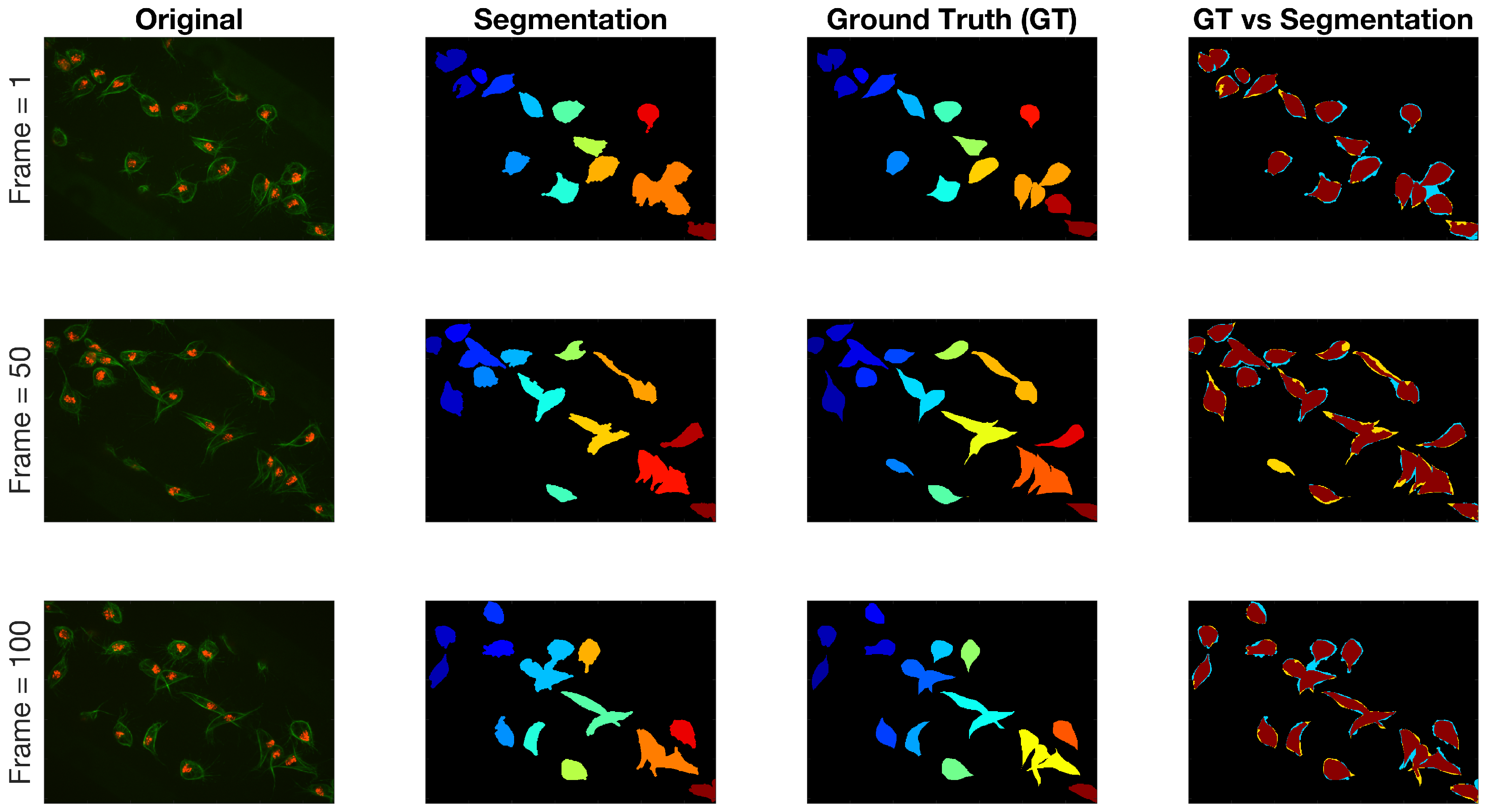
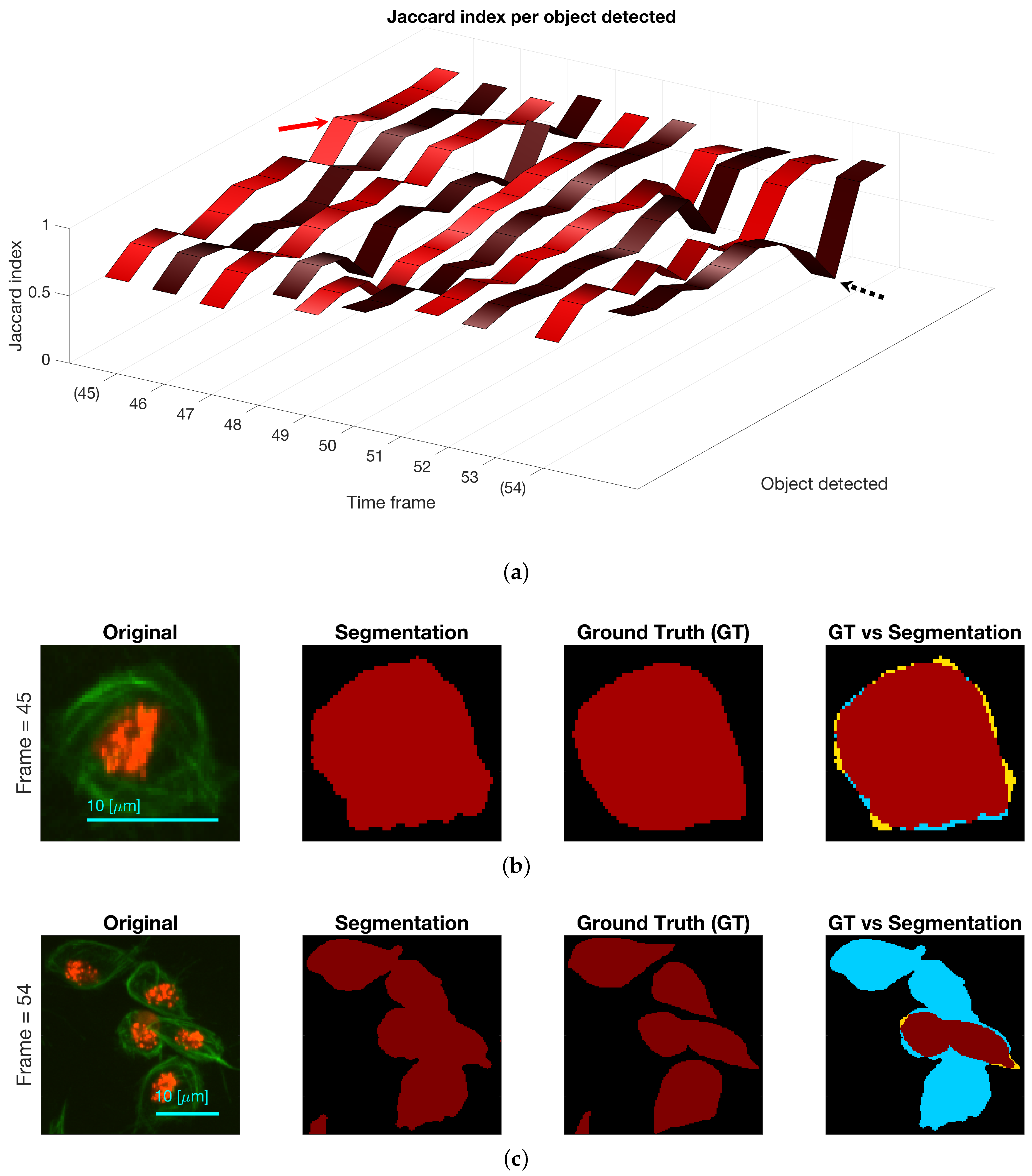
Regarding the results for the detection of objects, Figure 12 shows the detection of objects in the green channel (whether overlapping exists or not) on three representative frames of the dataset. A comparison with the ground truth (GT) is made on the far most right column, where black shows the background, yellow represent the false negatives, blue the false positives and red the true positives. The Jaccard Index per detected object was computed for all objects in the available frames. The results are shown in Figure 13, top, where the frame numbers are outlined along the axis. Two arrows were added to the figure to point a high Jaccard value (red), shown in the middle column of the figure and a notably low one (black - -), which corresponds to the bottom column.
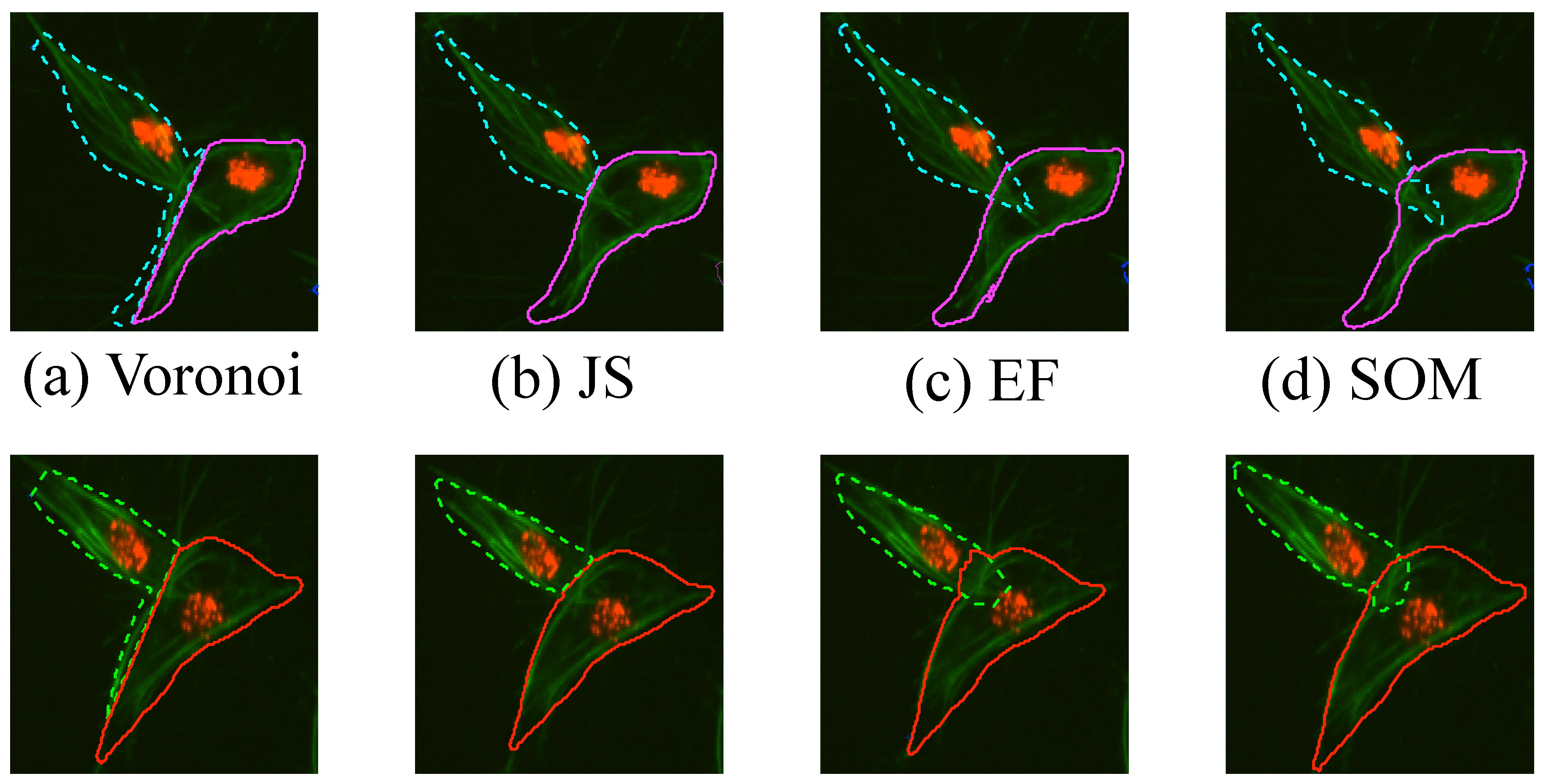
The results obtained for one frame of overlapping cells examined in detail are shown in Figure 14, which are two clumps that look similar throughout the images. Finally, a comparison with manually segmented ground truth was performed in ten frames. In order to have the best results shown for each of the methods, the input clumps used were taken from the ground truth images. Four methods of the segmentation of overlapping cells were explored, these methods are explained thoroughly in Section 2.4. Briefly, the segmentation methods are a naïve segmentation based in Voronoi tessellations [18]; then three methods that use the information from the detected junctions (bends): Junction Slicing (JS), Edge Following (EF) and Self-organising Maps (SOM). The Jaccard Similarity Index [21], recall and precision [22] statistics were computed for both clumps on all the frames and all the methods described, box plots of the results are shown in Figure 15 and summarised in Table 1. Table 2 presents a statistical analysis of the results presented in Table 1. The Wilcoxon Signed Rank test [23] was implemented to compare the results per measurement, for example Precision(Voronoi) vs. Precision(JS). The test was chosen as an alternative to a traditional t-test, without the need to assume the distribution of the measured values.
4. Discussion
Preliminary work using thresholding techniques [7], active contours [9,14] or multilevel set methods [11] did not provide satisfactory segmentation of the overlapping cells in single frames, as these techniques could only detect clusters of overlapping objects without distinction between them (data not shown). Statistical shape analysis methods have improved significantly from [24] to the recent [25]. However, newer techniques have not been applied to detect overlapping and would probably have to undergo further research. In [17], a method to segment overlapping cells by analysing the boundary of an overlapping clump was presented. In this paper, the method presented in [17] was extended by introducing the analysis of a single (non-overlapping) object. Its main advantage is to present a way to find relevant junctions from a boundary based on the angles alongside it, whether they are obtuse (bends) or acute (corners).
Limitations when detecting bends were found in the angle ranges of [188–192] degrees. The junction can be missed if the junction is not deep enough, this concept is clarified in Section 2.3. Figure 9 shows a correct detection on most of the cases presented, except in the upper left corner. The case of a separation of 0 pixels and an angle of 10 degrees shows one of the limitations, with an overdetection of junctions. In other cases, the junctions found would fall out of the 5 pixels range—and be classed as erroneous—or be missed altogether. The ellipses seem appropriate as a synthetic model for the overlapping of cells, since the segmented images (Figure 12) in most cases do not present irregular boundaries, which would alter the anglegram causing false detections. Figure 10 shows the performance of the method to detect corners when the only variation is in the pointiness. The method was able to detect the correct number of corners except in the case of a drop where two corners were detected. Figure 11 shows the junctions detected by the anglegram would not require further post-processing to select the useful junctions, unlike the Harris algorithm outputs. Since the junctions of interest would correspond to the intersection of the boundaries of the underlying cells, the assessment of them can be done qualitatively. Consistent with synthetic tests, limitations were observed in CLUMP 1, Figure 11a, where a junction was missed by both methods. This limitation depends on cell positions and is transferred to the underlying segmentation methods. Regardless of the overlapping the detection of objects in the green channel, Figure 12 and Figure 13, present some errors that need to be addressed, since the following methods depend on the detection of cells and clumps to be accurate. Table 1 shows a better performance from all three junction-based methods compared to the Voronoi partition. Furthermore, the percentile box sizes in Figure 15 show that the EF method (yellow) is less consistent than the SOM method (white).
5. Conclusions
In this work, the information extracted by the anglegram through the experimental results demonstrate the promise of the method to produce correct segmentations of overlapping cells, Figure 14. Single shape determination was presented as well, providing a baseline for shape analysis. Future work involves at least two foreseeable paths for development. In the case of bend detection, further experimentation is ongoing applying these techniques to cases where more than two main junctions are detected, such as the one presented in Figure 7a and cases where more than two cells are present in the clump. In the case of corners, a classification problem is being considered for shape identification and to provide a standardised scale to compare pointiness in shapes. This analysis would allow a connection of the shape’s pointiness to the migration patterns of the cells. In addition, the extension of the anglegram matrix as a prior to a probabilistic modelling of the position of the junctions and the overall shape is being considered.
Acknowledgments
This work was funded by a Doctoral Studentship granted by the School of Mathematics, Computer Science and Engineering at City, University of London.
Author Contributions
J.A.S.-L. and C.C.R.-A. conceived and designed the experiments; J.A.S.-L. performed the experiments; J.A.S.-L. , C.C.R.-A. and G.S. analysed the data; B.S. contributed the materials and motivation for this work; J.A.S.-L. wrote the paper and J.A.S.-L., C.C.R.-A., G.S. and B.S. revised the paper.
Conflicts of Interest
The authors declare no conflict of interest. The founding sponsors had no role in the design of the study; in the collection, analyses, or interpretation of data; in the writing of the manuscript, and in the decision to publish the results.
Abbreviations
The following abbreviations are used in this manuscript:
| EF | Edge Following |
| JS | Junction Slicing |
| MIP | Maximum Intensity Projection |
| mIP | Minimum Intensity Projection |
| ROI | Region of interest |
| SOM | Self-organising maps |
References
- Martinez, F.O.; Sica, A.; Mantovani, A.; Locati, M. Macrophage activation and polarization. Front. Biosci. J. Virtual Libr. 2008, 13, 453–461. [Google Scholar] [CrossRef]
- Wood, W.; Martin, P. Macrophage Functions in Tissue Patterning and Disease: New Insights from the Fly. Dev. Cell 2017, 40, 221–233. [Google Scholar] [CrossRef] [PubMed]
- Pocha, S.M.; Montell, D.J. Cellular and molecular mechanisms of single and collective cell migrations in Drosophila: Themes and variations. Ann. Rev. Genet. 2014, 48, 295–318. [Google Scholar] [CrossRef] [PubMed]
- Stramer, B.; Moreira, S.; Millard, T.; Evans, I.; Huang, C.Y.; Sabet, O.; Milner, M.; Dunn, G.; Martin, P.; Wood, W. Clasp-mediated microtubule bundling regulates persistent motility and contact repulsion in Drosophila macrophages in vivo. J. Cell Biol. 2010, 189, 681–689. [Google Scholar] [CrossRef] [PubMed] [Green Version]
- Maška, M.; Ulman, V.; Svoboda, D.; Matula, P.; Matula, P.; Ederra, C.; Urbiola, A.; España, T.; Venkatesan, S.; Balak, D.M.W.; et al. A benchmark for comparison of cell tracking algorithms. Bioinformatics (Oxford) 2014, 30, 1609–1617. [Google Scholar] [CrossRef] [PubMed]
- Ulman, V.; Maška, M.; Magnusson, K.E.G.; Ronneberger, O.; Haubold, C.; Harder, N.; Matula, P.; Matula, P.; Svoboda, D.; Radojevic, M.; et al. An objective comparison of cell-tracking algorithms. Nat. Methods 2017, 14, 1141–1152. [Google Scholar] [CrossRef] [PubMed]
- Henry, K.M.; Pase, L.; Ramos-Lopez, C.F.; Lieschke, G.J.; Renshaw, S.A.; Reyes-Aldasoro, C.C. PhagoSight: An Open-Source MATLAB® Package for the Analysis of Fluorescent Neutrophil and Macrophage Migration in a Zebrafish Model. PLoS ONE 2013, 8, e72636. [Google Scholar] [CrossRef] [PubMed]
- Dufour, A.; Shinin, V.; Tajbakhsh, S.; Guillén-Aghion, N.; Olivo-Marin, J.C.; Zimmer, C. Segmenting and tracking fluorescent cells in dynamic 3-D microscopy with coupled active surfaces. IEEE Trans. Image Process. 2005, 14, 1396–1410. [Google Scholar] [CrossRef] [PubMed]
- Chan, T.F.; Vese, L.A. Active contours without edges. IEEE Transa. Image Process. 2001, 10, 266–277. [Google Scholar] [CrossRef] [PubMed]
- Plissiti, M.E.; Nikou, C. Overlapping Cell Nuclei Segmentation Using a Spatially Adaptive Active Physical Model. IEEE Transa. Image Process. 2012, 21, 4568–4580. [Google Scholar] [CrossRef] [PubMed]
- Lu, Z.; Carneiro, G.; Bradley, A.P. An Improved Joint Optimization of Multiple Level Set Functions for the Segmentation of Overlapping Cervical Cells. IEEE Transa. Image Process. 2015, 24, 1261–1272. [Google Scholar]
- Reyes-Aldasoro, C.C.; Aldeco, A.L. Image segmentation and compression using neural networks. In Advances in Artificial Perception and Robotics; CIMAT: Guanajuato, Mexico, 2000; pp. 23–25. [Google Scholar]
- Hannah, I.; Patel, D.; Davies, R. The use of variance and entropic thresholding methods for image segmentation. Pattern Recognit. 1995, 28, 1135–1143. [Google Scholar] [CrossRef]
- Caselles, V.; Kimmel, R.; Sapiro, G. Geodesic Active Contours. Int. J. Comput. Vis. 1997, 22, 61–79. [Google Scholar] [CrossRef]
- Harris, C.; Stephens, M. A Combined Corner and Edge Detector. In Proceedings of the 4th Alvey Vision Conference Alvety Vision Club, University of Manchester, Manchester, UK, 31 August–2 September 1988; pp. 147–151. [Google Scholar]
- Lindeberg, T. Junction detection with automatic selection of detection scales and localization scales. In Proceedings of the 1st International Conference on Image Processing, Austin, TX, USA, 13–16 November 1994; Volume 1, pp. 924–928. [Google Scholar]
- Solís-Lemus, J.A.; Stramer, B.; Slabaugh, G.; Reyes-Aldasoro, C.C. Segmentation of Overlapping Macrophages Using Anglegram Analysis. In Communications in Computer and Information Science, Proceedings of the Medical Image Understanding and Analysis, Edinburgh, UK, 11–13 July 2017; Springer: Cham, Switzerland, 2017; pp. 792–803. [Google Scholar]
- Okabe, A.; Boots, B.; Sugihara, K.; Chiu, S.N.; Kendall, D.G. Algorithms for Computing Voronoi Diagrams. In Spatial Tessellations; John Wiley & Sons, Inc.: Hoboken, NJ, USA, 2000; pp. 229–290. [Google Scholar]
- Canny, J. A Computational Approach to Edge Detection. IEEE Trans. Pattern Anal. Mach. Intell. 1986, 8, 679–698. [Google Scholar] [CrossRef] [PubMed]
- Kohonen, T. The self-organizing map. Neurocomputing 1998, 21, 1–6. [Google Scholar] [CrossRef]
- Jaccard, P. Étude comparative de la distribution florale dans une portion des Alpes et des Jura. Bull. Soc. Vaud. Sci. Nat. 1901, 37, 547–579. [Google Scholar]
- Fawcett, T. An Introduction to ROC Analysis. Pattern Recognit. Lett. 2006, 27, 861–874. [Google Scholar] [CrossRef]
- Hollander, M.; Wolfe, D.A.; Chicken, E. The One-Sample Location Problem. In Nonparametric Statistical Methods; John Wiley & Sons, Inc.: Hoboken, NJ, USA, 2015; pp. 39–114. [Google Scholar]
- Cootes, T.F.; Taylor, C.J.; Cooper, D.H.; Graham, J. Active Shape Models-Their Training and Application. Comput. Vis. Image Underst. 1995, 61, 38–59. [Google Scholar] [CrossRef]
- Gooya, A.; Lekadir, K.; Castro-Mateos, I.; Pozo, J.M.; Frangi, A.F. Mixture of Probabilistic Principal Component Analyzers for Shapes from Point Sets. IEEE Trans. Pattern Anal. Mach. Intell. 2017, PP. [Google Scholar] [CrossRef] [PubMed]
Sample Availability: Samples of the data and the code used to compute the anglegram algorithm are available at https://github.com/alonsoJASL/matlab.anglegram, or upon request to the corresponding author. Also, the code to generate ground truth is available in https://github.com/alonsoJASL/matlab.manualSegmentation. |
Figure 1.
Two representative time frames displaying examples of cell shapes and overlapping. (a) Full frame with (red) squares highlighting the cells that display the aforementioned shapes; (b) Detail of each cell; (c) Presents the full frame with (red) squares highlighting all regions where instances of overlapping cells (clumps) are shown and labelled for easy reference; (d) Detail of CLUMP 2, present in (c). Bars: 10 μm. (c,d) are reproduced with permission from [17].

Figure 2.
Example of the ground truth at a representative time frame. The ground truth for both red (nuclei) and green (microtubules) channels is shown in coloured lines. The frame is shown in grey scale to allow for a better visualisation of the lines in the ground truth.
Figure 2.
Example of the ground truth at a representative time frame. The ground truth for both red (nuclei) and green (microtubules) channels is shown in coloured lines. The frame is shown in grey scale to allow for a better visualisation of the lines in the ground truth.

Figure 3.
Overview of the range of paired ellipses investigated. The pairs presented on this image represent a small sample of the ellipses that were tested by the method presented. The overlapped region can be seen in white and the areas that are not overlapping are shown in grey. The boundary of the central ellipse is highlighted in cyan while the second ellipse’s boundary is presented in red.

Figure 4.
Synthetic generation of random basic shapes. Per shape, 200 cases were generated. The control points are shown in blue (·). The mean shapes are presented in magenta (−); and the mean control points are represented in black (⋄).
Figure 4.
Synthetic generation of random basic shapes. Per shape, 200 cases were generated. The control points are shown in blue (·). The mean shapes are presented in magenta (−); and the mean control points are represented in black (⋄).


Figure 5.
Graphical representation of the calculation of the inner point angle of point at separation j. (a) Representation of the inner angle of point at separation j. Notice that the points in the boundary are taken in clockwise order; (b) Representation of the translation vectors . Full explanation in text.

Figure 6.
Explanation of inner angle of a point in the construction of the anglegram. The diagram shows a representation of nine arbitrary entries of the anglegram matrix. Each entry corresponds to an inner point angle at a specific separation. In the diagram, as in the matrix, the rows (i) correspond to a single point alongside the boundary (red ⋄) that start at a specific point (marked ○); the columns (j) correspond to the separation from the point i⋄ and from there the angle is taken. Each corresponding entry, , of the anglegram matrix is marked with a green arrow, furthermore, each angle is shaded to match the colour map used in the anglegram in Figure 7.

Figure 7.
Junction detection on overlapping objects through the maximum intensity projection of the anglegram matrix. (a–c) Representation of inner point angle calculation and generation of the anglegram matrix. (a) Represents a synthetic clump with its boundary outlined (blue - -), where a point (blue ○) in the boundary will have various inner point angles per separation j; All the inner point angles for the highlighted point are displayed in (b); (c) Shows the anglegram matrix, and the definition of is represented in (d) along the boundary points. Detection of junctions are shown with ⋄ markers (magenta). Notice the two horizontal lines representing and . [17] Reproduced with permission.

Figure 8.
Illustration of all the methods developed and the workflow to obtain results. (a) shows the detail of CLUMP 2 in the original frame. Clumps are detected and the boundary was extracted. With the boundary information, the anglegram was calculated and the junctions were detected (b). On the second row, a diagram to the methods were presented. From left to right, the (c) Voronoi partition, (d) Junction Slicing (JS), (e) Edge Following (EF) and (f) SOM fitting. In (g) the outputs from each method for both cells within the detected clump are shown. [17] Reproduced with permission.

Figure 9.
Junction (bends) detected for varying angles and separation distances. Five rows show angles ranging from 10 to 90 degrees and eight columns showing different separation distances from 0 to 160 pixels. Images in grey are cases where there is no overlap. The boundary of the clumps is shown in cyan (- -), with the first point in the boundary marked (⋄). The junctions detected by the method are marked in magenta ().

Figure 10.
Pointiness assessment of the drop, bidrop and tridrop shapes, see full explanation in text. For each shape presented, three instances of the shape are shown with varying pointiness values; the relationship of the anglegram and the pointiness is shown. The columns are arranged in triads corresponding to each of the basic shapes. Notice that, in all cases, the difference between the maximum and minimum values of the mIP (solid lines in third row) grows proportionally to the pointiness level.


Figure 11.
Qualitative comparison of junction detection via anglegram (magenta ⋄) versus the Harris corner detector (green +). The strongest corners from the Harris detector per clump are displayed. (a) Only CLUMP 1 has a missing junction (cyan ○), it should be noticed how difficult detection of the junction would be. [17] Reproduced with permission. (b) Each basic shape in the data is represented from a segmented frame. Refer to Section 2.3 for a full explanation of the corner detection algorithm.

Figure 12.
Qualitative comparison of segmentation technique against the ground truth on three different time frames in the dataset. The columns from left to right present the original image, the manual segmentation (GT), the result of the segmentation described in Section 2.4 and finally the comparison between both binary images. Regarding the colours in the final column: black is the background, yellow represent the false negatives, blue the false positives and red the true positives.

Figure 13.
(a) Comparison of the Jaccard index for each object detected, whether it is a clump or not, at each of the ten frames with available ground truth. Two frames are highlighted (45 and 54) and arrows point at values in the ribbon. (b) Depiction of cell in frame 45 that achieved a high Jaccard index in Top row (red arrow). (c) Depiction of clump detected in frame 54, and its comparison with the ground truth. The black dotted arrow in the top row show the Jaccard index value of the clump shown. Regarding the colours in the segmentation comparison: black is the background, yellow represent the false negatives, blue the false positives and red the true positives.

Figure 14.
Qualitative comparison of different segmentation methods in one frame. The segmentation results for (a) the Voronoi method, (b) Junction Slicing (JS), (c) Edge Following (EF) and (d) SOM fitting are shown. Top and Bottom rows represent the results for CLUMP 2 and CLUMP 3 respectively [17]. Reproduced with permission.

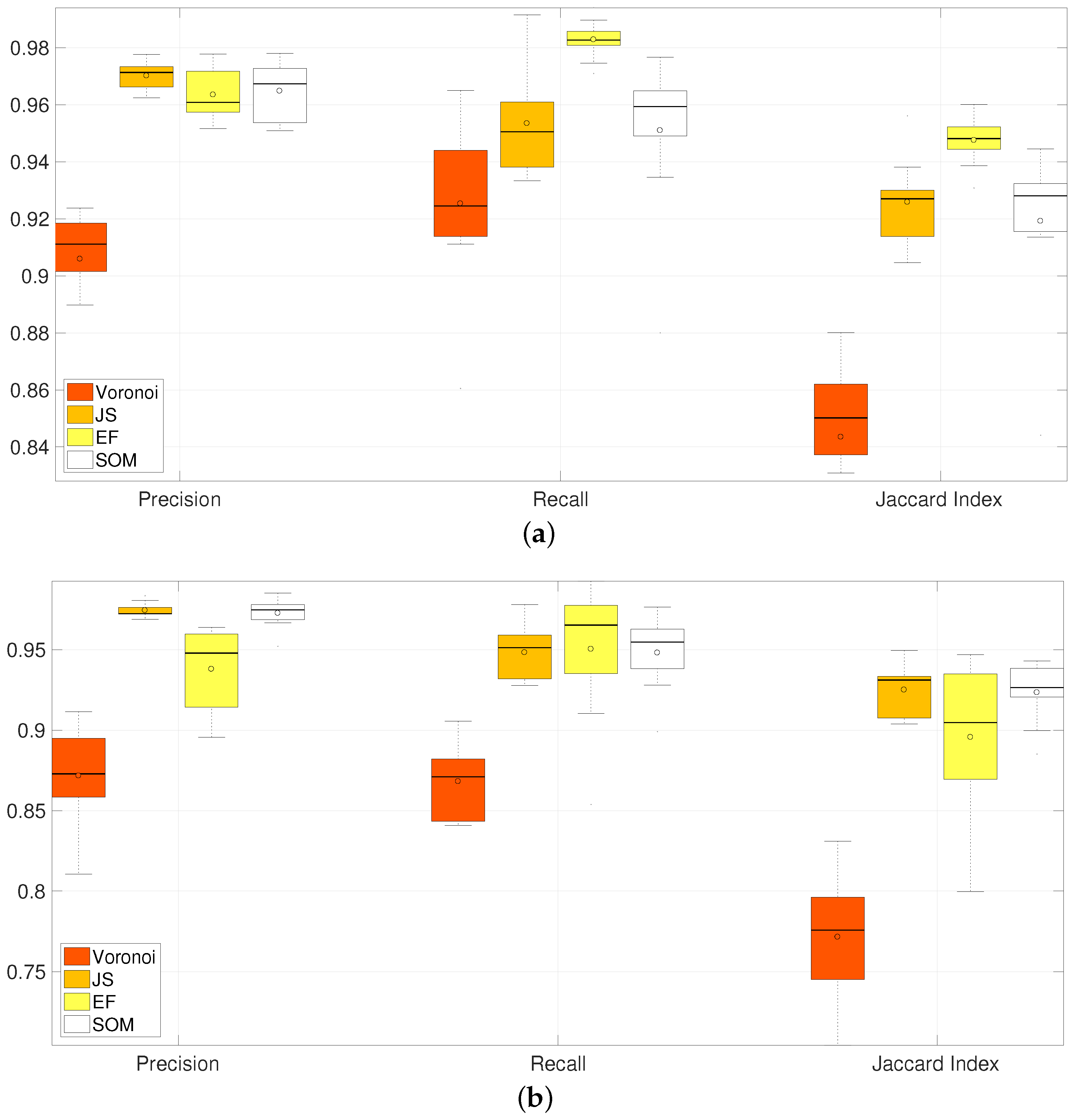
Figure 15.
Comparison of Precision, Recall and Jaccard Index for all methods of segmentation of overlapping in clumps 2 and 3. Horizontal axis correspond to the box plots from the different methods and their summarised performance in the metrics computed. Three groups corresponding to Precision, Recall and Jaccard Index contain four box plots; which, from left to right, correspond to Voronoi, JS, EF and SOM methods. Table 1 summarises the information on this image. [17] Reproduced with permission. (a) CLUMP 2. Y-axis ranges from ; (b) CLUMP 3. Y-axis ranges from .


Table 1.
Comparison of mean values of Precision, Recall and Jaccard Index for clumps 2 and 3 over 10 frames. This table summarises the results in Figure 14. Highest results are highlighted.
Table 1.
Comparison of mean values of Precision, Recall and Jaccard Index for clumps 2 and 3 over 10 frames. This table summarises the results in Figure 14. Highest results are highlighted.
| CLUMP 2 | CLUMP 3 | |||||
|---|---|---|---|---|---|---|
| Precision | Recall | Jaccard Index | Precision | Recall | Jaccard Index | |
| Voronoi | 0.906 | 0.925 | 0.843 | 0.872 | 0.868 | 0.771 |
| JS | 0.970 | 0.953 | 0.926 | 0.974 | 0.948 | 0.925 |
| EF | 0.964 | 0.983 | 0.948 | 0.938 | 0.950 | 0.896 |
| SOM | 0.965 | 0.951 | 0.919 | 0.973 | 0.948 | 0.923 |
Table 2.
Statistical analysis of results presented in Table 1. The Wilcoxon Signed Rank test [23] was implemented to compare the results per measurement (Voronoi, JS, EF and SOM). The table presents the p-values on the paired test for each of the pairs, (first and second columns). Tests where the null hypothesis could not be rejected are highlighted.
| CLUMP 2 | CLUMP 3 | ||||||
|---|---|---|---|---|---|---|---|
| Precision | Recall | Jaccard Index | Precision | Recall | Jaccard Index | ||
| Voronoi vs. | JS | ||||||
| EF | |||||||
| SOM | |||||||
| JS vs. | EF | ||||||
| SOM | |||||||
| EF vs. | SOM | ||||||
© 2017 by the authors. Licensee MDPI, Basel, Switzerland. This article is an open access article distributed under the terms and conditions of the Creative Commons Attribution (CC BY) license (http://creativecommons.org/licenses/by/4.0/).
Share and Cite
MDPI and ACS Style
Solís-Lemus, J.A.; Stramer, B.; Slabaugh, G.; Reyes-Aldasoro, C.C. Segmentation and Shape Analysis of Macrophages Using Anglegram Analysis. J. Imaging 2018, 4, 2. https://0-doi-org.brum.beds.ac.uk/10.3390/jimaging4010002
AMA Style
Solís-Lemus JA, Stramer B, Slabaugh G, Reyes-Aldasoro CC. Segmentation and Shape Analysis of Macrophages Using Anglegram Analysis. Journal of Imaging. 2018; 4(1):2. https://0-doi-org.brum.beds.ac.uk/10.3390/jimaging4010002
Chicago/Turabian StyleSolís-Lemus, José Alonso, Brian Stramer, Greg Slabaugh, and Constantino Carlos Reyes-Aldasoro. 2018. "Segmentation and Shape Analysis of Macrophages Using Anglegram Analysis" Journal of Imaging 4, no. 1: 2. https://0-doi-org.brum.beds.ac.uk/10.3390/jimaging4010002
Note that from the first issue of 2016, this journal uses article numbers instead of page numbers. See further details here.