A Non-Structural Representation Scheme for Articulated Shapes

Department of Computer Engineering, Middle East Technical University, Ankara 06800, Turkey
*
Author to whom correspondence should be addressed.
J. Imaging 2018, 4(10), 115; https://0-doi-org.brum.beds.ac.uk/10.3390/jimaging4100115
Submission received: 4 September 2018
/
Revised: 27 September 2018
/
Accepted: 2 October 2018
/
Published: 8 October 2018
Abstract
:Articulated shapes are successfully represented by structural representations which are organized in the form of graphs of shape components. We present an alternative representation scheme which is equally powerful but does not require explicit modeling or discovery of structural relations. The key element in our scheme is a novel multi scale pixel-based distinctness measure which implicitly quantifies how rare a particular pixel is in terms of its geometry with respect to all pixels of the shape. The spatial distribution of the distinctness yields a partitioning of the shape into a set of regions. The proposed representation is a collection of size normalized probability distribution of the distinctness over regions over shape dependent scales. We test the proposed representation on a clustering task.
1. Introduction
Shape is a distinguishing attribute of an object frequently utilized in image processing and computer vision applications. Measuring the similarity of objects via their shapes is a challenging task due to high within-class and low between-class variations. Within-class variations may be due to transformations such as rotation, scaling, and motion of limbs or independent motion of parts called articulations. Among within-class variations, articulations pose a particular challenge in the sense that articulations can not be modeled as global transformation groups. Hence, one can not define proper global descriptors that are invariant to articulations. Nevertheless, shapes of objects that articulate (referred to as articulated shapes) can be successfully represented by structural representations which are organized in the form of graphs of shape components. These components can be branches or critical points of the shape skeleton, subsets of the shape interior (commonly referred as parts), or fragments of shape boundary (commonly referred as contour fragments). Among many works in the literature that address shape similarity via structural representations, some examples are [1,2,3,4,5,6,7,8]. Skeleton based structural representations are the the most common ones; extensive literature reviews can be found in several works, e.g., [2,9].
In this work, we develop a novel representation scheme for articulated shapes. The representation scheme is not structural, i.e., it does not explicitly model components and their relationships. Our main argument against structural representations is that it is challenging to extract components and their structural relationships. Moreover, measuring similarity of shapes through their structural representations requires finding a correspondence between a pair of graphs, which is an intricate process necessitating advanced algorithms.
The strength of our representation lies in two factors. First, multiple characterizations of the shape are extracted based on descriptive and complementary shape scales. Second, each point in the shape communicates to the remaining points in the shape, thereby gaining an emergent role with respect to the remaining. We call this emergent role distinctness. The distinctness yields a partitioning of the shape into a set of regions, and the shape regions are described via size normalized probability distribution of the distinctness associated with their constituent points. Ultimately, our final representation is a collection of size normalized probability distribution of the distinctness over regions and over scales.
In order to evaluate the new representation, we use it for shape clustering. The clustering results obtained on three articulated shape datasets show that our method performs comparable to state of the art methods utilizing component graphs or trees, even though we are not explicitly modeling component relations.
Clustering or unsupervised grouping of shapes is a fundamental problem addressed in the literature. In [10], hierarchical clustering is applied where the closest pair of clusters is merged at each step. A common structure skeleton graph is constructed for each cluster and the distance between the clusters is determined by matching their associated graphs. In [11], spectral clustering is employed for fusing the similarity measures obtained via skeleton-based and contour-based shape descriptors. In [12], the distance of shapes is measured using a new shape descriptor obtained by extending a contour-based descriptor to the shape interior and multi-objective optimization is applied to determine both the number of clusters and an optimal clustering result. In [13], shape is represented via the distances from the centroid of the shape to the boundary points and a nonlinear projection algorithm is applied to group together similar shapes. In [14], geodesic path constructed between differential geometric representations of the shape boundaries is used for hierarchical clustering of shapes. In [15], elastic properties of the shape boundaries are considered and clustering is applied based on the elastic geodesic distance with dynamic programming alignment. In [16], a new distance measure that is defined between a single shape and a group of shapes is utilized in a soft k-means like clustering of shapes.
2. The Method
2.1. The Proposed Representation and Its Construction
We explain the process in four steps. First, we construct a multi-scale feature for each pixel where the scales are determined as multiples of a shape dependent number (Section 2.1.1). As we consider a large number of scales (say 30), this gives a high dimensional representation. The values at all pixels are computed simultaneously via a relaxation procedure meaning that the pixels influence each other. In this respect, and its multiples implicitly determine the extent of interaction among neighboring pixels.
Second, we vary how we select the shape dependent number in order to obtain several high dimensional representations (Section 2.1.2). The motivation here is to robustly capture the proper shape scale. A novelty in the way we vary is the introduction of two complementary base shape scales (Section 2.1.2).
Third, at each , we form feature matrix , where each row represents the feature vector computed for a shape pixel and m is the total number of shape pixels. D is later decomposed into a low-rank matrix L and a sparse matrix S. The norm of the corresponding vector in the matrix S is the key element for our representation, namely distinctness (of the respective shape pixel) (Section 2.1.3).
Fourth, spatial distribution of the distinctness is used to partition the shape into a set of regions and region-wise normalized distinctness density functions (probability density for distinctness) are estimated (Section 2.1.4). The collection of regional distinctness density functions form the final representation.
2.1.1. Construction of the High-Dimensional Feature Space
Consider a planar shape discretized using a grid of dimension . We construct a 30-dimensional feature vector for each shape pixel , where and . In order to compute the feature component at each slot k for , we first solve a linear system of equations in which the feature value of each shape pixel is related with the feature values of its four-neighboring pixels via (1) and we then normalize the obtained values as in (2).
is solved only for the shape pixels, and it is considered 0 for the pixels outside the shape. is a scalar parameter which controls the dependence between the feature value of each shape pixel and the feature values of its four-neighbors.
In Figure 1 (left), we show the features computed for a one-dimensional signal using three different values of corresponding to , , and 1 multiples of the signal length. We normalize each feature to have the maximum value of 1 (see Figure 1 (right)). We observe that the feature values monotonically increase towards the center.
By varying , we obtain a collection of features each encoding a different degree of local interaction between the shape pixels and their surroundings. We determine for as , where represents the extent of the maximum interaction between the shape pixels and their surroundings. We organize the 30 features for each pixel in the form of a matrix , where m is the total number of shape pixels.
2.1.2. Complementary Shape Scales and Multiple High-Dimensional Feature Spaces
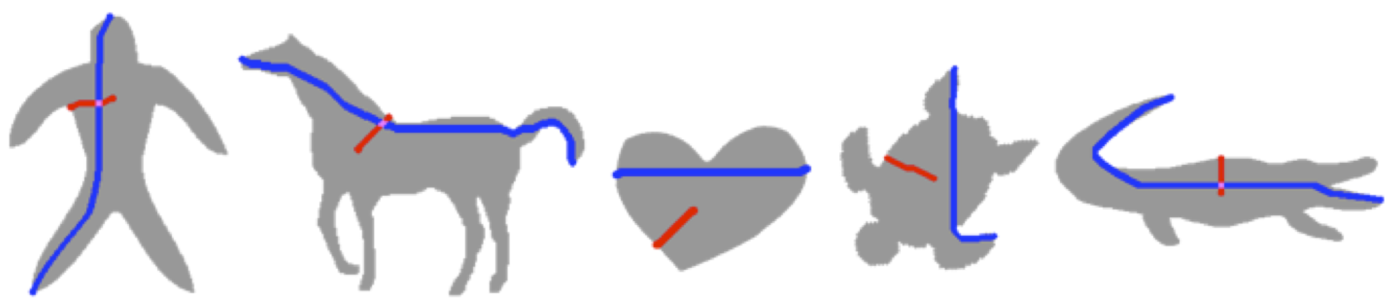
The question is how to select . In order to represent different shapes in a common feature space, we should determine for each shape individually in terms of a shape scale. But, how do we compute the proper shape scale? Our solution is to utilize two complementary base shape scales which are related with thickness of the shape body and the maximum distance between the shape extremities. The first scale R is computed as the maximum value of the shape’s distance transform, which gives the distance of each shape point from the nearest boundary. The second scale G is computed as the maximum value of the pairwise geodesic distances between the boundary points, where the geodesic distance between a pair of points depends on the shortest path connecting them through the shape domain.
As shown in Figure 2, R and G provide characteristic shape information which can be used to define the extent of the local interactions between the shape pixels during the feature space construction. We construct six different feature spaces, for which is selected as multiples of R or G.
2.1.3. Computing Distinctness
Recall that we organized the feature vectors in the form of a matrix , where each row represents the feature vector computed for a shape pixel. The matrix D is decomposed into a low-rank matrix L and a sparse matrix S via Robust Principal Component Analysis (RPCA), which seeks to solve the following convex optimization problem:
where denotes the sum of the singular values of the matrix, is the sum of the absolute values of all matrix entries, and is the weight of penalizing denseness of the sparse matrix S. Various algorithms are proposed to solve the optimization problem in (3). We use the inexact augmented Lagrange multipliers method for RPCA [17], which is efficient and highly accurate. We choose , as suggested by the available implementation of [17].
The low rank component L is expected to encode correlations among the shape pixels via their feature values, whereas the sparse component S is expected to encode their discriminations as it contains the residuals stemming from less frequent feature configurations. Thus, we define the distinctness of each shape pixel as the norm of the corresponding vector in the matrix S. The shape pixels whose feature components vary more are found to be more distinct.
The shape articulations are associated with larger distinctness since they are thinner compared to the shape body and the constant value coming from the shape boundary is propagated faster in these regions during the feature computation. We use these characteristics of the distinctness to partition shapes into a set of regions.
2.1.4. The Final Representation
A simple thresholding based on the mean distinctness yields two disjoint sets. With the exception of isolated tiny regions or thin strips near boundary, the two disjoint sets correspond to central (below-mean) and peripheral (above-mean) regions, respectively. We will denote them with C and P. At a large , P might be a single connected component. As decreases, C grows. The mean value based thresholding readily provides quite an intuitive split of the shape domain.
For consistency, we need to eliminate above-mean locations that appear in the inner regions and below-mean locations that occur in the outer regions. These are misclassified pixels: Whereas the above-mean locations that appear in the inner regions are misclassified as belonging to P, the below-mean locations that appear in the outer regions are misclassified as belonging to C. Thus, we perform an adaptive morphological processing. Specifically, we sequentially dilate P and then C by adaptively choosing the radius of the structuring element at each pixel as the shortest distance of the pixel to the nearest boundary. Before the adaptive dilation, a pre-correction step to correct misclassified the inner pixels is useful. This is because we are performing dilation on P before C. In our implementation, we detected a misclassified component as the above-mean component of which minimum distance to the boundary is more than a quarter of the shape radius R. The adaptive dilation process corrects misclassified locations to a large extent. Whereas the adaptive dilation of P removes below-mean components in P and merges nearby above-mean components, the adaptive dilation of the new C (pixels surviving P dilation) merges nearby below-mean components, reducing the number of connected components in C. The dilation of C has a side effect. It generally causes the split of P into subsets corresponding to different limbs. Of course due to boundary roughness (noise or texture), the process may also create distractive small components.
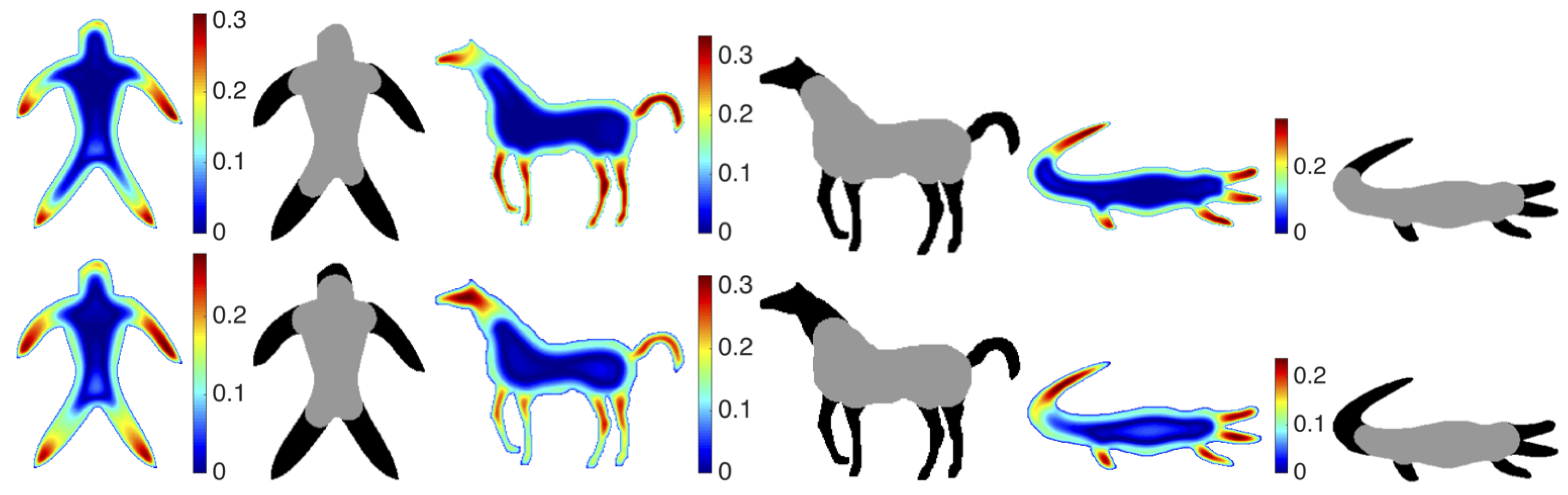
Hence, a secondary correction process is further useful. The purpose is to eliminate very small peripheral regions and to force the shape to have a single center unless it is composed of multiple blobs of comparable size. In our implementation, in the the secondary correction process, below-mean components that are smaller than of the area of the largest below-mean component are marked as peripheral, and above-mean components that are smaller than of the shape area are marked as central. In Figure 3, results for two values are shown. At the selected scales, surviving regions seem to be quite intuitive.
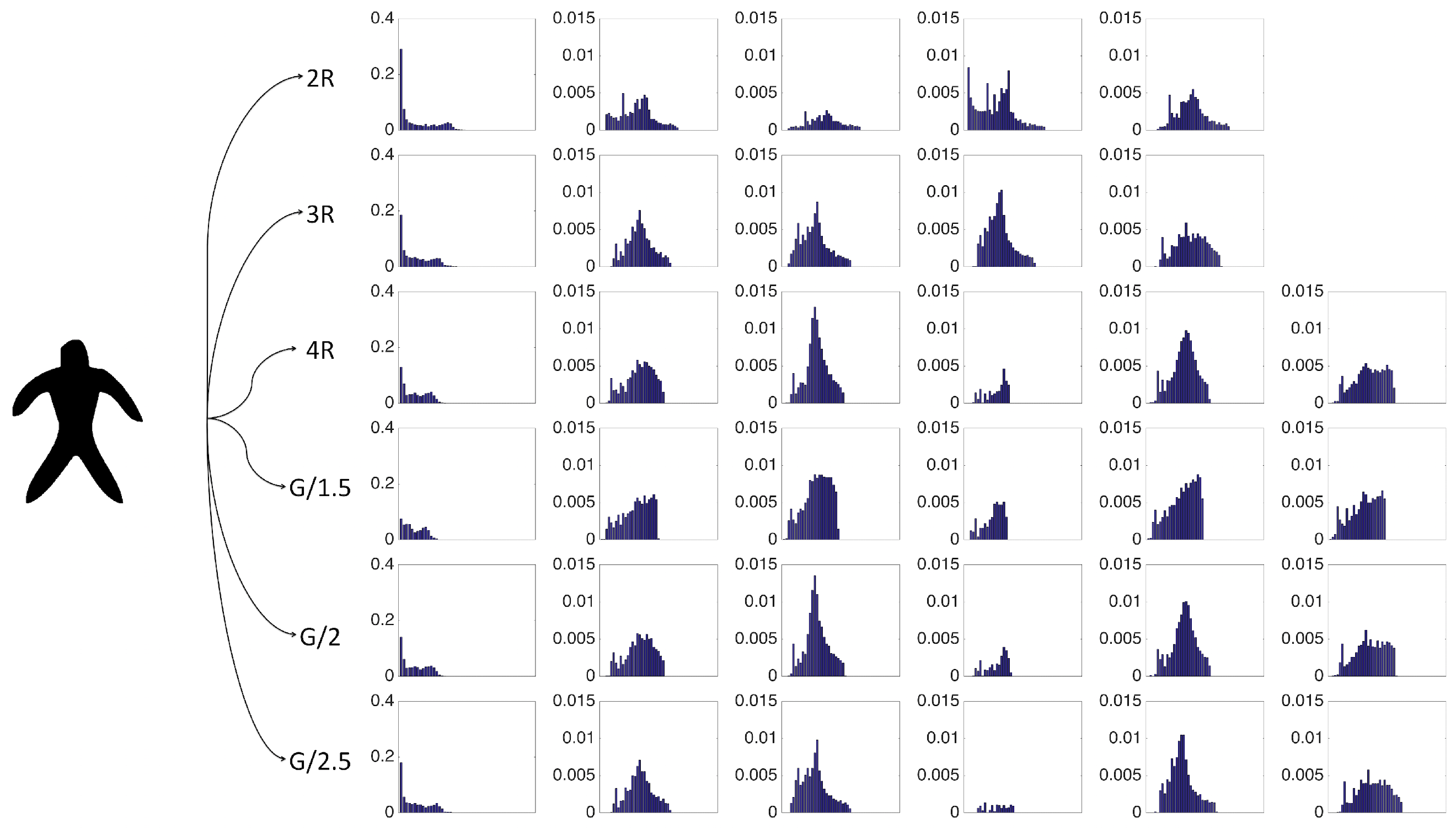
The final representation is a collection of regions-wise normalized density functions. A single distribution is constructed for the central region, whereas separate distributions are constructed for each of the surviving peripheral regions. The region-wise normalization is performed by making the cumulative probability equal to the ratio of the respective region area to the total shape area. The scales are determined by choosing as , , , , , and . A demonstration is given in Figure 4. Notice that values based on R are increasing as they are multiplied with factors larger than 1, whereas values based on G are decreasing as they are divided. This is not a coincidence: R corresponds to an inner shape scale implying the minimum extent of interaction required between the shape pixels, whereas G corresponds to an outer scale implying the maximum extent of interaction.
2.2. Clustering Shapes
We use pairwise dissimilarities derived from our shape representation as features for clustering. Let the number of shapes in the dataset be N. Then, N × N dissimilarity matrix (whose construction is described in Section 2.2.1) enables to associate each shape with an N-dimensional feature vector of which components denote pairwise dissimilarities between the respective shape and all the N shapes in the dataset. We map all NN-dimensional feature vectors to a plane using t-Distributed Stochastic Neighbor Embedding (t-SNE) [18], which is a powerful dimensionality reduction tool. It captures the local structure of the data points in the original dimension and maps them to nearby points in the reduced dimension space.
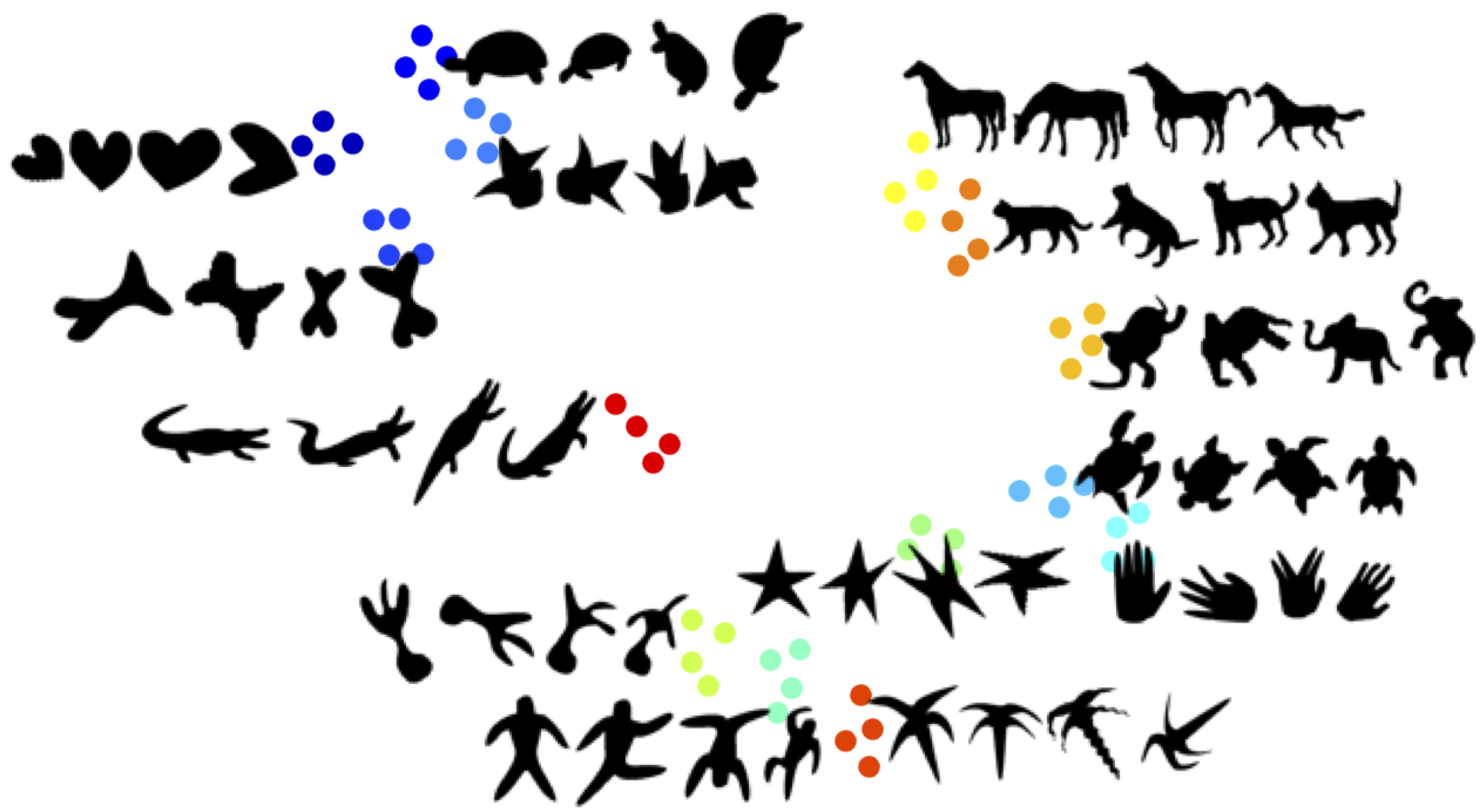
In Figure 5, we show the t-SNE mapping result for the dataset [3] where the within category variations are due to transformations such as rotation, scaling, and deformations of articulations. We see that the shapes from the same category cluster together and the shapes from the similar categories (e.g., horse and cat shapes) are close to each other.
Given two-dimensional coordinates of the shapes obtained via t-SNE mapping, we once more compute the pairwise distances; this time, between the points in the plane. Then we apply affinity propagation [19] to partition the dataset into a number of clusters (which is chosen as equal to the number of categories in the set). The affinity propagation is a relaxation procedure for exchanging real-valued messages between the data points until a high-quality set of exemplars and corresponding clusters gradually emerges. The default affinity is negated Euclidean distance. We experiment with several other distances.
2.2.1. Measuring Pairwise Shape Dissimilarity
The dissimilarity between a pair of shapes at a given scale is defined as the cost of the optimal assignment between the shape regions (using the normalized distinctness density functions). We use Hungarian matching for solving the optimal assignment problem. We do not assume any relation between the regions of each shape. Hungarian matching aims to find a one-to-one correspondence between the regions of the two shapes leaving some regions unmatched. The cost of assigning two regions is simply taken as the distance between their normalized density functions. The cost of leaving a region unmatched is taken as the norm of its normalized density function. We experimented with different distance metrics (Section 3), and the norm is computed suitably. For example, if the metric is city block, the cost becomes the proportion of the unmatched parts area. We define the final pairwise shape dissimilarity as a weighted average of the dissimilarities deduced from the six scales. The dissimilarities via the scales depending on R are weighted as three times the dissimilarities via the scales depending on G. The non-uniform weighting is due to that R is more reliable than G, since the shape body is a more stable structure compared to the articulations.
3. Experimental Evaluation
In order to evaluate clustering results, we used Normalized Mutual Information (NMI). NMI measures the degree of agreement between the ground-truth category partition and the obtained clustering partition by utilizing the entropy measure. Let denote the number of shapes in cluster i and category j, denote the number of shapes in cluster i, and denote the number of shapes in category j. Then, NMI can be computed as follows:
where I is the number of clusters, J is the number of categories, and N is the total number of shapes. Notice that a high value of NMI indicates that the obtained clustering result matches well with the ground-truth category partition. We experimented with three shape datasets [2,3,5]. These are the most articulated datasets in the literature. The first dataset [3] consists of 14 shape categories each with 4 shapes, the second dataset [2] consists of 30 categories each with 6 shapes, and the third dataset [5] consist of 50 categories each with 20 shapes.
The easiest method of estimating a probability density function is constructing a histogram; an alternative is kernel density estimation (KDE). For comparing probability distributions, a proper distance should be used. Nevertheless, for simplicity we will use city block distance. To make sure that our choices for density estimation method and comparison metric are good, we performed an experiment to compare the chosen combination against the remaining three alternatives. Of course, for experiments, we also need to choose a metric for the final affinity propagation process. We considered four different metrics, hence experimented with settings for each of the 3 datasets (yielding a total of NMIs (Table 1)). Results support the following conclusions. First, for probability distribution estimation, there is no significant difference between the two methods; hence, it is wiser to choose the simpler one, i.e., estimating via histogram (Observe that NMI values only slightly decrease when kernel density estimation is used). Second, for histogram comparison, city block distance is a better alternative. For histogram construction, the bin size is set to 0.01.
A side observation is that all four tested metrics for the affinity propagation seemed to perform comparably. In the next experiment, we enlarged the set of possibilities to 12. NMIs are reported in Table 2. With the exception of distance, the metrics seemed to perform comparably.
3.1. Comparison to State of the Art Methods
In Table 3, we compare NMIs of the state of the art methods of which performances are reported for the considered datasets. The CSD (common structure discovery) [10] employs hierarchical clustering; a common shape structure is constructed each time two clusters are merged into a single cluster. Building a common shape structure requires matching skeletons. The method (skeleton+spectral) [11] combines the skeleton path distance [4] with spectral clustering. The performance of these two skeleton-based methods decreases for the third dataset which contains unarticulated shape categories such as face category. For this data set, the highest performance is obtained via the method (contour+spectral) [11] which uses the shape context descriptor [20]. As the shape context descriptor [20] is not robust to articulations, its performance is lower for the highly articulated first and second datasets. We also report averaged NMIs. In each of the two groups, the first column is the ordinary average whereas the second and third are weighted averages. The weighting is according to total number of categories and total number of shapes, respectively. Our distinctness based method accurately clusters the first set. For the second and the third dataset, respectively, NMIs are at least 99% and 95% of the best score.
Notice that the method in the fifth row (combining Inner Distance Shape Context (IDSC) descriptor IDSC [22] with normalized cuts) exhibits obviously inferior performance. The NMIs are taken from [10]. IDSC is not a structural method; the core idea is to build histogram descriptors from pairwise geodesic distance measurements among all boundary points. The expectation is that geodesic distances will be articulation invariant. There are also several other geodesic distance based shape descriptors, one of which is the so called eccentricity transform [23]. To compare our distinctness based representation to the geodesic distance based representation in [23], we performed 36 tests by varying the choice of metric and the dataset. The results are summarized in in Table 4. Each reported statistics is estimated using 6 NMIs. There seems to be a clear performance difference between the two representations. In order to make sure the observed difference in performance is significant in the sense that it can not be explainable via within group variation as in use of different metric (as in Table 2), we performed p-test. Based on the p-test, the probability of observing the observed difference in mean due to within group variance is calculated to be zero (Table 5). Dataset specific values are obtained by pooling the standard deviations for distinctness (Table 2) and for eccentricity. We used the available implementation of the eccentricity transform given in [24] and selected the parameters as . These are the parameter values reported in [23].
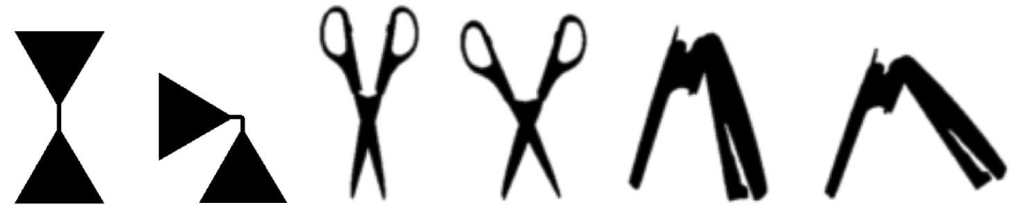
An articulated object is a union of parts and junctions. In the literature, some authors define articulations as transformations that are rigid when restricted to a part. Bending invariant geodesic distance based measures seem to work in a restricted setting when joints are small compared to parts and part transformation are rigid. Figure 6 shows few sample shapes on which the geodesic distance based methods (e.g., [22,23]) are tested.
3.2. Representing Shapes Using a Single Histogram for Distinctness
In our proposed scheme, each shape is represented by a collection of regional histograms. A simpler alternative is to skip the partitioning step and represent the shape using a single histogram estimated using all of the distinctness values. In Table 6, we report the clustering performance when shapes are represented by a single global histogram instead of a collection of regional histograms. For each of the three sets, the higher performance is marked as bold. Even when the shape is represented only using a single histogram, the discrepancy outperforms eccentricity.
4. Summary and Conclusions
We proposed a new representation along with a clustering scheme to group articulated shapes in terms of similarity. The proposed representation is based on a novel multi-scale, pixel-wise distinctness measure. Our experiments show that the distinctness density (both region-wise or global) is a robust descriptor. A distinctness based clustering scheme is shown to perform comparably to the state of the art methods based on structural representations; the scheme even outperforms as the degree of articulations/deformations increase. In comparison to geodesic-distance based representations, proposed representation brings significant performance improvement. As a side property, the spatial distribution of the distinctness provides easy partitioning of the shape domain into regions. Though at some scales these regions seem to be intuitive, at some other scales they do not. At some scales, there may be only a single region. We remark that we neither intend to obtain shape segmentation nor intend to obtain part hierarchy; the key point is that the distinctness implicitly codes structural relations.
Author Contributions
A.G. and S.T. contributed to the design and development of the proposed method and to the writing of the manuscript. A.G. contributed additionally to the software implementation and testing of the proposed method.
Funding
This research was funded by TUBITAK grant number 112E208.
Conflicts of Interest
The authors declare no conflict of interest. The funding sponsors had no role in the design of the study; in the collection, analyses, or interpretation of data; in the writing of the manuscript, and in the decision to publish the results.
Abbreviations
| 2D | Two-dimensional |
| RPCA | Robust Principal Component Analysis |
| t-SNE | t-Distributed Stochastic Neighbor Embedding |
| NMI | Normalized Mutual Information |
References
- Akimaliev, M.; Demirci, M.F. Improving skeletal shape abstraction using multiple optimal solutions. Pattern Recognit. 2015, 48, 3504–3515. [Google Scholar] [CrossRef]
- Aslan, C.; Erdem, A.; Erdem, E.; Tari, S. Disconnected skeleton: Shape at its absolute scale. IEEE Trans. Pattern Anal. Mach. Intell. 2008, 30, 2188–2203. [Google Scholar] [CrossRef] [PubMed]
- Aslan, C.; Tari, S. An axis-based representation for recognition. In Proceedings of the 2005 International Conference on Computer Vision, Beijing, China, 17–20 October 2005. [Google Scholar]
- Bai, X.; Latecki, L. Path Similarity Skeleton Graph Matching. IEEE Trans. Pattern Anal. Mach. Intell. 2008, 30, 1282–1292. [Google Scholar] [CrossRef] [PubMed] [Green Version]
- Baseski, E.; Erdem, A.; Tari, S. Dissimilarity between two skeletal trees in a context. Pattern Recognit. 2009, 42, 370–385. [Google Scholar] [CrossRef] [Green Version]
- Super, B.J. Knowledge-based part correspondence. Pattern Recognit. 2007, 40, 2818–2825. [Google Scholar] [CrossRef]
- Wang, C.; Lai, Z. Shape decomposition and classification by searching optimal part pruning sequence. Pattern Recognit. 2016, 54, 206–217. [Google Scholar] [CrossRef]
- Yang, C.; Tiebe, O.; Shirahama, K.; Grzegorzek, M. Object matching with hierarchical skeletons. Pattern Recognit. 2016, 55, 183–197. [Google Scholar] [CrossRef]
- Saha, P.K.; Borgefors, G.; di Baja, G.S. A survey on skeletonization algorithms and their applications. Pattern Recognit. Lett. 2016, 76, 3–12. [Google Scholar] [CrossRef]
- Shen, W.; Wang, Y.; Bai, X.; Wang, H.; Latecki, L. Shape clustering: Common structure discovery. Pattern Recognit. 2013, 46, 539–550. [Google Scholar] [CrossRef]
- Bai, S.; Liu, Z.; Bai, X. Co-spectral for robust shape clustering. Pattern Recognit. Lett. 2016, 83, 388–394. [Google Scholar] [CrossRef]
- Liu, R.; Wang, R.; Yu, X.; An, L. Shape automatic clustering-based multi-objective optimization with decomposition. Mach. Vis. Appl. 2017, 28, 497–508. [Google Scholar] [CrossRef]
- Yankov, D.; Keogh, E. Manifold Clustering of Shapes. In Proceedings of the Sixth International Conference on Data Mining (ICDM’06), Hong Kong, China, 18–22 December 2006. [Google Scholar]
- Srivastava, A.; Joshi, S.H.; Mio, W.; Liu, X. Statistical shape analysis: Clustering, learning, and testing. IEEE Trans. Pattern Anal. Mach. Intell. 2005, 27, 590–602. [Google Scholar] [CrossRef] [PubMed]
- Mio, W.; Srivastava, A.; Joshi, S. On Shape of Plane Elastic Curves. Int. J. Comput. Vis. 2007, 73, 307–324. [Google Scholar] [CrossRef]
- Lakaemper, R.; Zeng, J. A Context Dependent Distance Measure for Shape Clustering. In Advances in Visual Computing; Bebis, G., Boyle, R., Parvin, B., Koracin, D., Remagnino, P., Porikli, F., Peters, J., Klosowski, J., Arns, L., Chun, Y.K., et al., Eds.; Springer: Berlin/Heidelberg, Germany, 2008; pp. 145–156. [Google Scholar]
- Lin, Z.; Chen, M.; Ma, Y. The augmented Lagrange multiplier method for exact recovery of corrupted low-rank matrices. arXiv, 2010; arXiv:1009.5055. [Google Scholar]
- van der Maaten, L.; Hinton, G. Visualizing High-Dimensional Data Using t-SNE. J. Mach. Learn. Res. 2008, 9, 2579–2605. [Google Scholar]
- Frey, B.J.; Dueck, D. Clustering by Passing Messages Between Data Points. Science 2007, 315, 972–976. [Google Scholar] [CrossRef] [PubMed] [Green Version]
- Belongie, S.; Malik, J.; Puzicha, J. Shape matching and object recognition using shape contexts. IEEE Trans. Pattern Anal. Mach. Intell. 2002, 24, 509–522. [Google Scholar] [CrossRef] [Green Version]
- Erdem, A.; Torsello, A. A Game Theoretic Approach to Learning Shape Categories and Contextual Similarities. In Structural, Syntactic, and Statistical Pattern Recognition; Hancock, E.R., Wilson, R.C., Windeatt, T., Ulusoy, I., Escolano, F., Eds.; Springer: Berlin/Heidelberg, Germany, 2010; pp. 139–148. [Google Scholar]
- Ling, H.; Jacobs, D.W. Shape Classification Using the Inner-Distance. IEEE Trans. Pattern Anal. Mach. Intell. 2007, 29, 286–299. [Google Scholar] [CrossRef] [PubMed] [Green Version]
- Ion, A.; Artner, N.M.; Peyré, G.; Kropatsch, W.G.; Cohen, L.D. Matching 2D and 3D articulated shapes using the eccentricity transform. Comput. Vis. Image Underst. 2011, 115, 817–834. [Google Scholar] [CrossRef] [Green Version]
- Peyre, G. Toolbox Fast Marching. 2009. Available online: https://www.mathworks.com/matlabcentral/fileexchange/6110-toolbox-fast-marching?s_tid=prof_contriblnk (accessed on 12 April 2016).
Figure 1.
Features computed for a one-dimensional signal using three different values of the parameter (left) and normalized features (right).
Figure 1.
Features computed for a one-dimensional signal using three different values of the parameter (left) and normalized features (right).

Figure 2.
R and G correspond to the thickness of the shape body (red) and the maximum distance between the shape extremities (blue), respectively.
Figure 2.
R and G correspond to the thickness of the shape body (red) and the maximum distance between the shape extremities (blue), respectively.

Figure 3.
Distinctness values (color coded) and the corresponding mean-value based partitioning (gray vs. black) for three shapes via the feature spaces constructed for (top row) and (bottom row). As decreases, gray regions grow.
Figure 3.
Distinctness values (color coded) and the corresponding mean-value based partitioning (gray vs. black) for three shapes via the feature spaces constructed for (top row) and (bottom row). As decreases, gray regions grow.

Figure 4.
The final representation as a collection of size normalized probability distributions over regions over six scales. The first distribution at each scale describes the central region. There is no ordering between the remaining distributions describing the peripheral regions.
Figure 4.
The final representation as a collection of size normalized probability distributions over regions over six scales. The first distribution at each scale describes the central region. There is no ordering between the remaining distributions describing the peripheral regions.

Figure 5.
t-SNE mapping of the shapes from the dataset [3] where the points with the same color denote the shapes from the same category.
Figure 5.
t-SNE mapping of the shapes from the dataset [3] where the points with the same color denote the shapes from the same category.

Figure 6.
Some sample shapes on which geodesic distance based methods are tested. In the literature, some authors [22,23] define articulations as transformations that are rigid when restricted to a part.


Table 1.
Comparing (HIS + City block) against the other three options. The experiment is repeated for four varying choices of metric for affinity propagation.
Table 1.
Comparing (HIS + City block) against the other three options. The experiment is repeated for four varying choices of metric for affinity propagation.
| ChebychevP | EuclideanP | |||||
|---|---|---|---|---|---|---|
| Set 1 | Set 2 | Set 3 | Set 1 | Set 2 | Set 3 | |
| HIS + City block + p = 2 | 1.0000 | 0.9651 | 0.9203 | 1.0000 | 0.9553 | 0.9172 |
| HIS + Euclidean + p = 2 | 1.0000 | 0.9464 | 0.8953 | 1.0000 | 0.9484 | 0.8958 |
| KDE + City block + p = 2 | 1.0000 | 0.9476 | 0.9025 | 1.0000 | 0.9476 | 0.9053 |
| KDE + Euclidean + p = 2 | 0.9453 | 0.9495 | 0.8817 | 0.9678 | 0.9454 | 0.8868 |
| HIS + City block + p = 1 | 0.9839 | 0.9651 | 0.9205 | 1.0000 | 0.9651 | 0.9177 |
| HIS + Euclidean + p = 1 | 0.9839 | 0.9367 | 0.8953 | 1.0000 | 0.9477 | 0.8941 |
| KDE + City block + p = 1 | 1.0000 | 0.9553 | 0.9015 | 1.0000 | 0.9575 | 0.9027 |
| KDE + Euclidean + p = 1 | 0.9453 | 0.9482 | 0.8872 | 0.9678 | 0.9482 | 0.8901 |
Table 2.
Normalized mutual information (NMI) values for different affinity propagation distances.
| p = 2 | p = 1 | |||||
|---|---|---|---|---|---|---|
| Set 1 | Set 2 | Set 3 | Set 1 | Set 2 | Set 3 | |
| EuclideanP | 1.0000 | 0.9553 | 0.9172 | 1.0000 | 0.9651 | 0.9177 |
| Standardized EuclideanP | 0.9839 | 0.9528 | 0.9170 | 0.9839 | 0.9528 | 0.9129 |
| MahalanobisP | 0.9534 | 0.9528 | 0.9142 | 0.9534 | 0.9528 | 0.9091 |
| City blockP | 0.9839 | 0.9560 | 0.9102 | 0.9839 | 0.9651 | 0.9109 |
| ChebychevP | 1.0000 | 0.9651 | 0.9203 | 0.9839 | 0.9651 | 0.9205 |
| CosineP | 0.9031 | 0.8428 | 0.7530 | 0.9031 | 0.8504 | 0.7601 |
| max | 1.0000 | 0.9651 | 0.9203 | 1.0000 | 0.9651 | 0.9205 |
| mean | 0.9707 | 0.9374 | 0.8886 | 0.9681 | 0.9419 | 0.8885 |
| std | 3.7% | 4.7% | 6.7% | 3.5% | 4.5% | 6.3% |
| std excluding CosineP | 1.9% | 0.5% | 0.4% | 1.7% | 0.7% | 0.5% |
Table 3.
Comparison of our clustering results with the state of the art methods using NMI. The best scores are marked as bold. Red and blue colors in the last two rows indicate a clustering result of which NMI is 99% and 95% of the best score.
Table 3.
Comparison of our clustering results with the state of the art methods using NMI. The best scores are marked as bold. Red and blue colors in the last two rows indicate a clustering result of which NMI is 99% and 95% of the best score.
| Set 1 | Set 2 | Set 3 | Avg (Set 1, Set 2) | Avg (Set 1, Set 2, Set 3) | |||||
|---|---|---|---|---|---|---|---|---|---|
| CSD [10] | 0.9734 | 0.9694 | 0.8096 | 0.9714 | 0.9707 | 0.9703 | 0.9175 | 0.8850 | 0.8403 |
| Skeleton+spectral [11] | 0.9426 | 0.9746 | 0.9154 | 0.9586 | 0.9644 | 0.9670 | 0.9442 | 0.9383 | 0.9253 |
| Contour+spectral [11] | 0.9418 | 0.9264 | 0.9676 | 0.9341 | 0.9313 | 0.9301 | 0.9453 | 0.9506 | 0.9604 |
| Skeleton+learning [21] | - | - | 0.8722 | - | - | - | - | - | - |
| IDSC+Ncuts [10,22] | 0.5660 | 0.5423 | 0.5433 | 0.5542 | 0.5498 | 0.5479 | 0.5505 | 0.5464 | 0.5442 |
| Our method (Euclidean) | 1.0000 | 0.9651 | 0.9177 | 0.9826 | 0.9762 | 0.9734 | 0.9609 | 0.9451 | 0.9283 |
| Our method (Chebychev2) | 1.0000 | 0.9651 | 0.9203 | 0.9826 | 0.9762 | 0.9734 | 0.9618 | 0.9465 | 0.9304 |
Table 4.
Distinctness versus eccentricity [23]. Each reported statistics is estimated using 6 NMIs. In each comparison, the higher performance is marked as bold.
Table 4.
Distinctness versus eccentricity [23]. Each reported statistics is estimated using 6 NMIs. In each comparison, the higher performance is marked as bold.
| Set 1 | Set 2 | Set 3 | |||||||
|---|---|---|---|---|---|---|---|---|---|
| Min | Max | Mean | Min | Max | Mean | Min | Max | Mean | |
| Eccentricity p = 2 | 0.7332 | 0.8227 | 0.7985 | 0.7588 | 0.8599 | 0.8360 | 0.6143 | 0.7457 | 0.7177 |
| Distinctness p = 2 | 0.9031 | 1.0000 | 0.9707 | 0.8428 | 0.9651 | 0.9374 | 0.7530 | 0.9203 | 0.8886 |
| Eccentricity p = 1 | 0.7309 | 0.8227 | 0.7981 | 0.7582 | 0.8620 | 0.8406 | 0.6088 | 0.7497 | 0.7180 |
| Distinctness p = 1 | 0.9031 | 1.0000 | 0.9681 | 0.8504 | 0.9651 | 0.9419 | 0.7601 | 0.9205 | 0.8885 |
Table 5.
p-test for NMI differences. Pooled standard deviations are used.
| 99% CI | 99% CI | |||||
|---|---|---|---|---|---|---|
| Min Δ | Max Δ | Mean Δ | (12 Sample) | (1 Sample) | p-Value (Mean) | |
| set 1 () | 0.131 | 0.217 | 0.171 | 0.024 | 0.084 | 0.000 |
| set 2 () | 0.084 | 0.110 | 0.101 | 0.027 | 0.095 | 0.000 |
| set 3 () | 0.139 | 0.185 | 0.171 | 0.038 | 0.131 | 0.000 |
Table 6.
Single histogram distinctness. For each of the three sets, the higher performance is marked as bold.
Table 6.
Single histogram distinctness. For each of the three sets, the higher performance is marked as bold.
| Set 1 | Set 2 | Set 3 | |
|---|---|---|---|
| Distinctness (single histogram) | 0.9678 | 0.9175 | 0.8381 |
| Eccentricity | 0.8227 | 0.8620 | 0.7413 |
© 2018 by the authors. Licensee MDPI, Basel, Switzerland. This article is an open access article distributed under the terms and conditions of the Creative Commons Attribution (CC BY) license (http://creativecommons.org/licenses/by/4.0/).
Share and Cite
MDPI and ACS Style
Genctav, A.; Tari, S. A Non-Structural Representation Scheme for Articulated Shapes. J. Imaging 2018, 4, 115. https://0-doi-org.brum.beds.ac.uk/10.3390/jimaging4100115
AMA Style
Genctav A, Tari S. A Non-Structural Representation Scheme for Articulated Shapes. Journal of Imaging. 2018; 4(10):115. https://0-doi-org.brum.beds.ac.uk/10.3390/jimaging4100115
Chicago/Turabian StyleGenctav, Asli, and Sibel Tari. 2018. "A Non-Structural Representation Scheme for Articulated Shapes" Journal of Imaging 4, no. 10: 115. https://0-doi-org.brum.beds.ac.uk/10.3390/jimaging4100115
Note that from the first issue of 2016, this journal uses article numbers instead of page numbers. See further details here.