Incorporating Surface Elevation Information in UAV Multispectral Images for Mapping Weed Patches

 , , ,
, , ,
Abstract
:1. Introduction
2. Materials and Methods
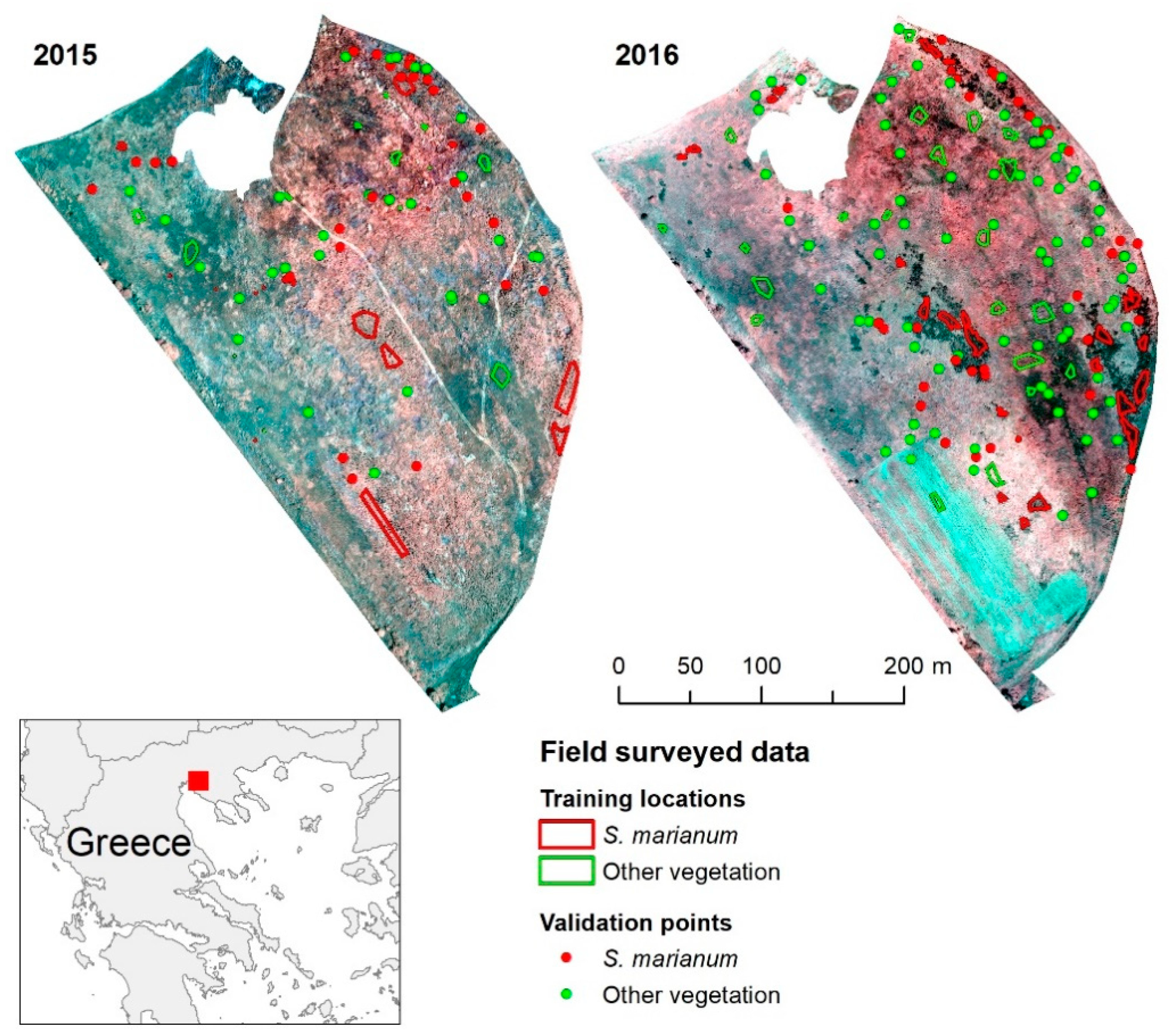
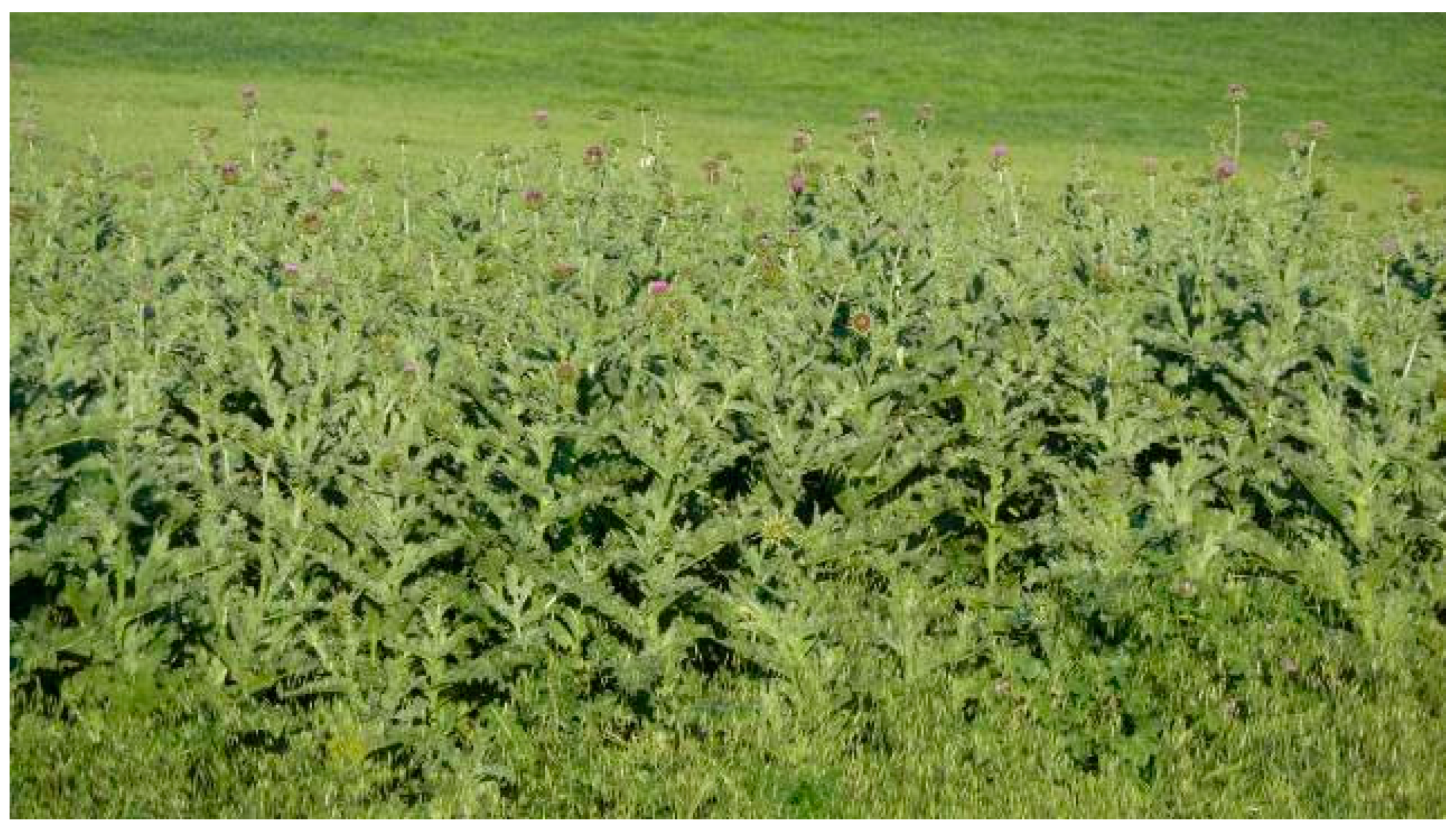
2.1. Study Area
2.2. Data
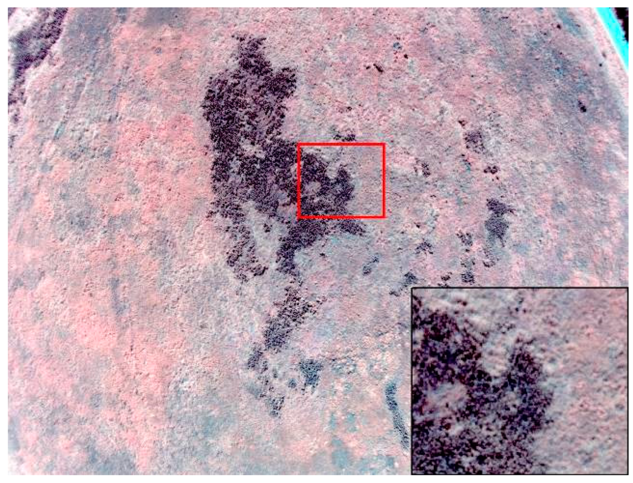
2.2.1. UAV Data
2.2.2. In-Situ Data
2.3. Digital Image Processing and Geographic Analysis
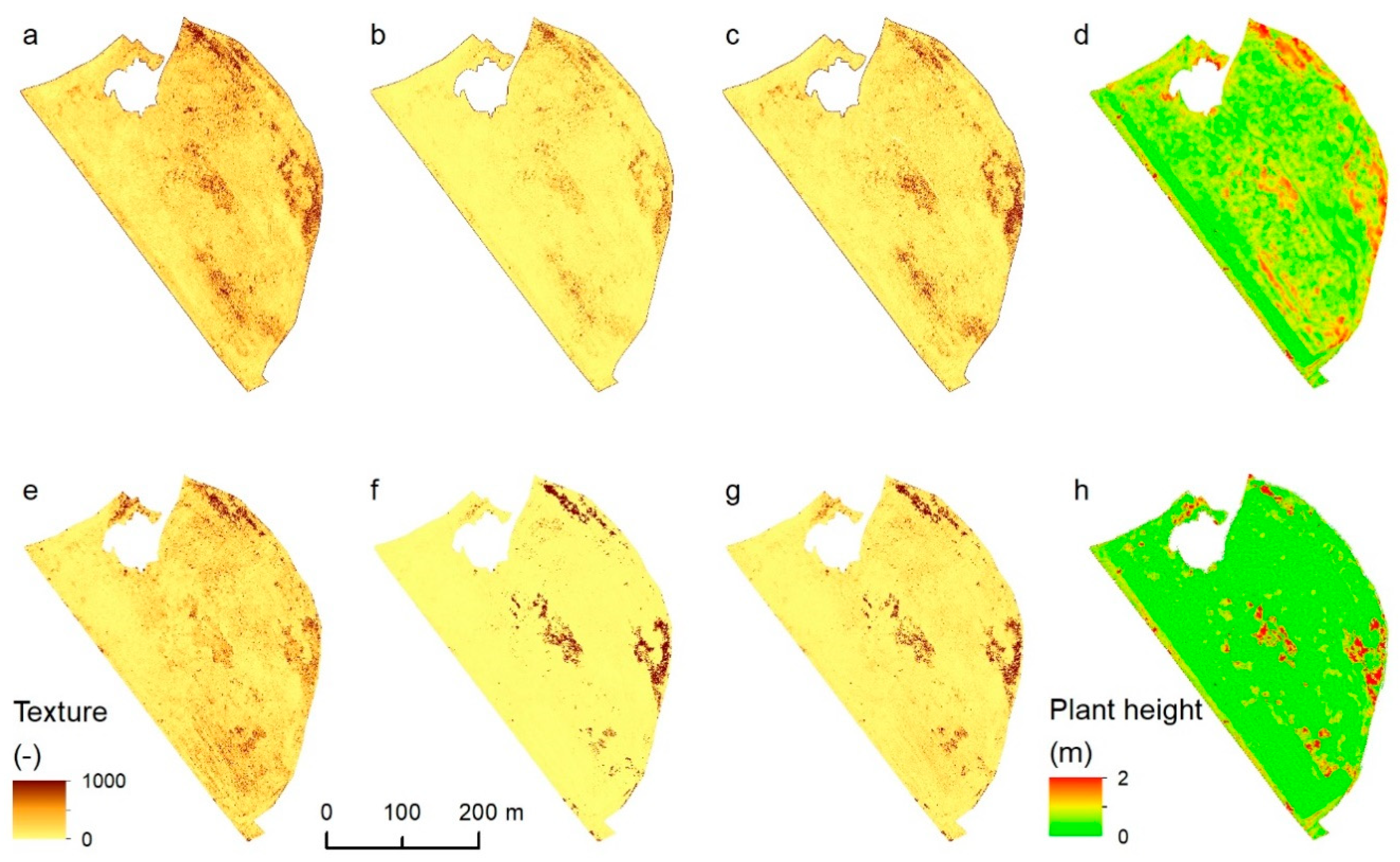
2.3.1. Surface Elevation Information and Texture
2.3.2. Image Classification and Accuracy Assessment
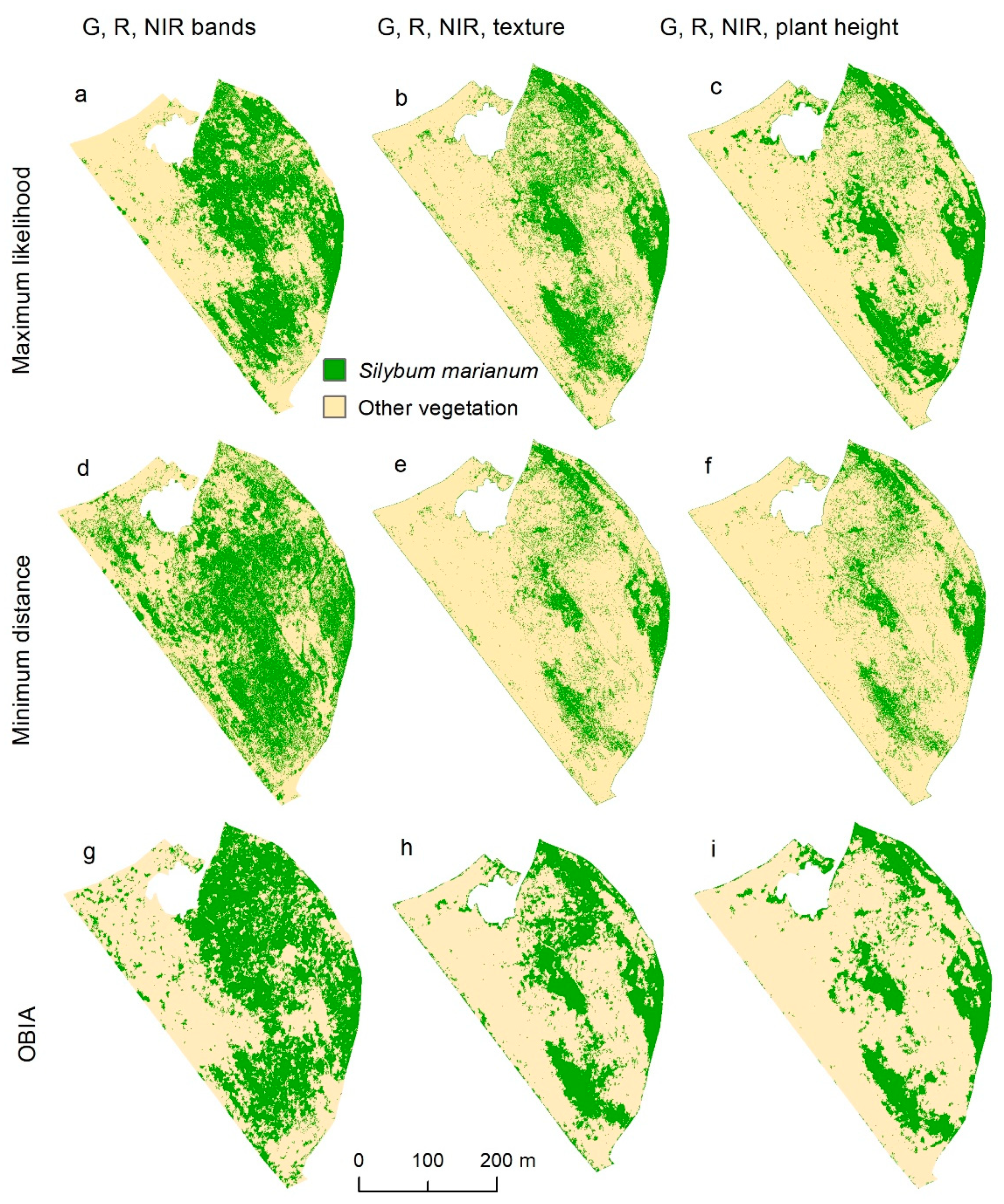
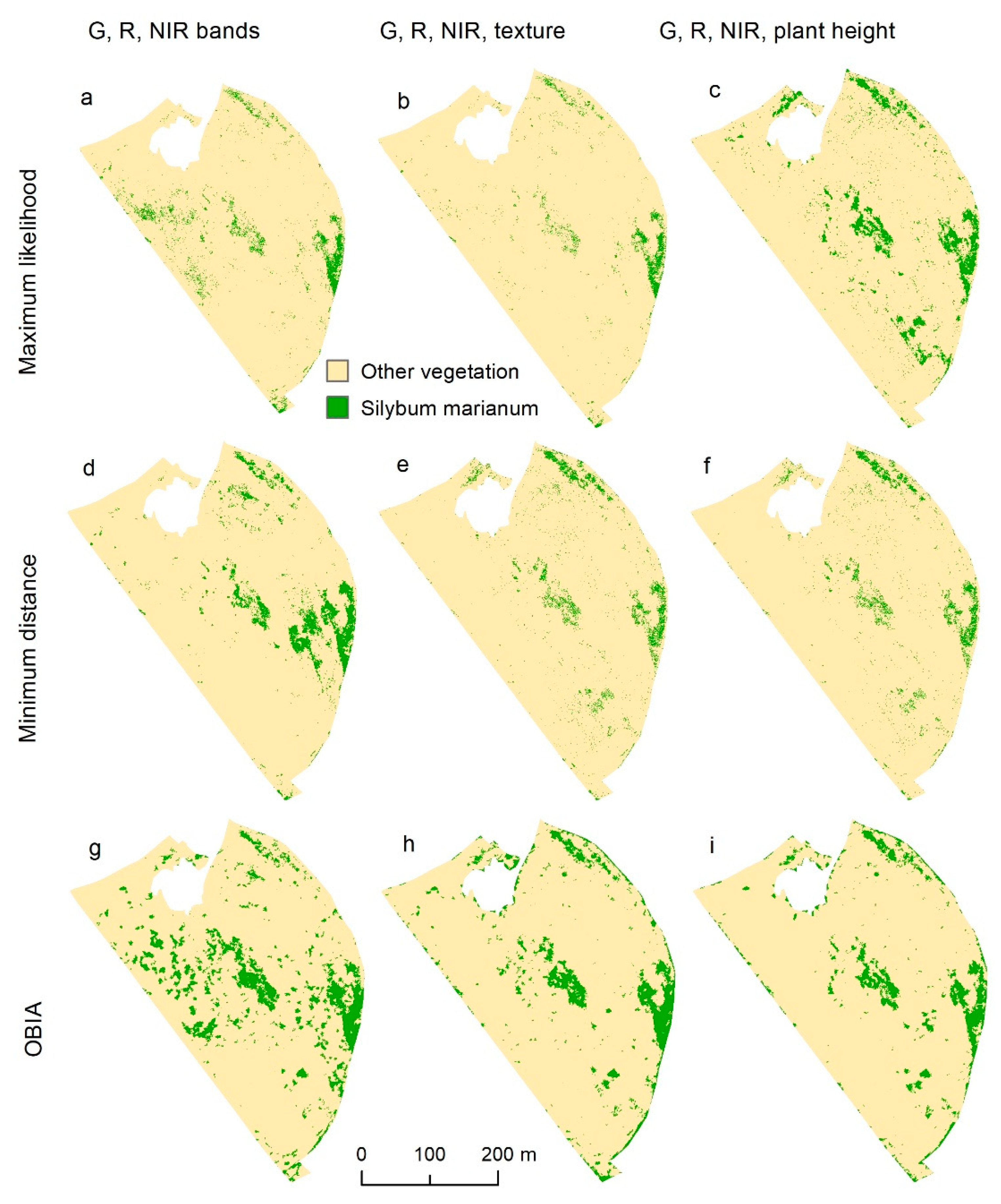
- The maximum likelihood (ML) algorithm is based on the assessment of the likelihood of a pixel belonging to a specific category. This method uses the data of the training areas for the assessment of the class centres, and the coexistence of the spectral classes are used to estimate probabilities. In addition to average values, the variability of reflectance values of each spectral class is considered.
- The minimum distance (MD) algorithm uses the median vectors of each pure pixel class from training areas (centre of each spectral class) and calculates the Euclidean distance of each unknown pixel to each centre. Pixels are classified to the nearest centre unless a standard deviation or threshold is set.
- For the object-based image analysis (OBIA), the commercial software eCognition Developer 9.0 (Trimble GeoSpatial, Munich, Germany) was used. To create the object-oriented environment, segmentation was applied using the ‘multiresolution segmentation’ algorithm on a 40 scale, which was more appropriate after testing for the size of the weed patches. The parameters for determining object homogeneity, that is, shape and compactness, were assigned the values 0.1 and 1, respectively, which produced objects in a more meaningful way [23]. Classification of objects was done using the nearest neighbour algorithm [24]. The in-situ collected samples were assigned into objects that defined the classes of interest. The mean values of each input layer were used appropriately as the features for each respective case of object-based classification. The algorithm uses the distance between the features’ range of values for the object being classified with the features’ range of values for the classes of interest, to define the membership degree to each class and eventually assign the object to a class.
3. Results
4. Discussion
5. Conclusions
Author Contributions
Funding
Acknowledgments
Conflicts of Interest
References
- Anderson, W. Weed Science, 3rd ed.; Waveland Press Inc.: Long Grove, IL, USA, 1996. [Google Scholar]
- Puri, V.; Nayyar, A.; Raja, L. Agriculture drones: A modern breakthrough in precision agriculture. J. Stat. Manag. Syst. 2017, 20, 507–518. [Google Scholar] [CrossRef]
- Peña, J.M.; Torres-Sánchez, J.; de Castro, A.I.; Kelly, M.; López-Granados, F. Weed mapping in early-season maize fields using object-based analysis of unmanned aerial vehicle (UAV) images. PLoS ONE 2013, 8, e77151. [Google Scholar] [CrossRef] [PubMed]
- Torres-Sánchez, J.; Peña, J.; de Castro, A.; López-Granados, F. Multi-temporal mapping of the vegetation fraction in early-season wheat fields using images from UAV. Comput. Electron. Agric. 2014, 103, 104–113. [Google Scholar] [CrossRef] [Green Version]
- Thorp, K.; Tian, L. A review on remote sensing of weeds in agriculture. Precis. Agric. 2004, 5, 477–508. [Google Scholar] [CrossRef]
- Castaldi, F.; Pelosi, F.; Pascucci, S.; Casa, R. Assessing the potential of images from unmanned aerial vehicles (UAV) to support herbicide patch spraying in maize. Precis. Agric. 2017, 18, 76–94. [Google Scholar] [CrossRef]
- Peña, J.; Torres-Sánchez, J.; Serrano-Pérez, A.; de Castro, A.; López-Granados, F. Quantifying efficacy and limits of unmanned aerial vehicle (UAV) technology for weed seedling detection as affected by sensor resolution. Sensors 2015, 15, 5609–5626. [Google Scholar] [CrossRef] [PubMed]
- Tamouridou, A.A.; Alexandridis, T.K.; Pantazi, X.E.; Lagopodi, A.L.; Kashefi, J.; Moshou, D. Evaluation of UAV imagery for mapping silybum marianum weed patches. Int. J. Remote Sens. 2017, 38, 2246–2259. [Google Scholar] [CrossRef]
- Pantazi, X.E.; Tamouridou, A.A.; Alexandridis, T.K.; Lagopodi, A.L.; Kashefi, J.; Moshou, D. Evaluation of hierarchical self-organising maps for weed mapping using UAS multispectral imagery. Comput. Electron. Agric. 2017, 130, 224–230. [Google Scholar] [CrossRef]
- Pérez-Ortiz, M.; Peña, J.M.; Gutiérrez, P.A.; Torres-Sánchez, J.; Hervás-Martínez, C.; López-Granados, F. Selecting patterns and features for between-and within-crop-row weed mapping using UAV-imagery. Expert Syst. Appl. 2016, 47, 85–94. [Google Scholar] [CrossRef]
- Gebhardt, S.; Kühbauch, W. A new algorithm for automatic rumex obtusifolius detection in digital images using colour and texture features and the influence of image resolution. Precis. Agric. 2007, 8, 1–13. [Google Scholar] [CrossRef]
- López-Granados, F.; Torres-Sánchez, J.; Serrano-Pérez, A.; de Castro, A.I.; Mesas-Carrascosa, F.-J.; Peña, J.-M. Early season weed mapping in sunflower using UAV technology: Variability of herbicide treatment maps against weed thresholds. Precis. Agric. 2016, 17, 183–199. [Google Scholar] [CrossRef]
- Küng, O.; Strecha, C.; Beyeler, A.; Zufferey, J.-C.; Floreano, D.; Fua, P.; Gervaix, F. The Accuracy of Automatic Photogrammetric Techniques on Ultra-Light UAV Imagery; UAV-g 2011-Unmanned Aerial Vehicle in Geomatics; ETH: Zurich, Switzerland, 2011. [Google Scholar]
- Zarco-Tejada, P.J.; Diaz-Varela, R.; Angileri, V.; Loudjani, P. Tree height quantification using very high resolution imagery acquired from an unmanned aerial vehicle (UAV) and automatic 3d photo-reconstruction methods. Eur. J. Agron. 2014, 55, 89–99. [Google Scholar] [CrossRef]
- Colomina, I.; Molina, P. Unmanned aerial systems for photogrammetry and remote sensing: A review. ISPRS J. Photogramm. Remote Sens. 2014, 92, 79–97. [Google Scholar] [CrossRef]
- Li, W.; Niu, Z.; Chen, H.; Li, D.; Wu, M.; Zhao, W. Remote estimation of canopy height and aboveground biomass of maize using high-resolution stereo images from a low-cost unmanned aerial vehicle system. Ecol. Indic. 2016, 67, 637–648. [Google Scholar] [CrossRef]
- Holman, F.H.; Riche, A.B.; Michalski, A.; Castle, M.; Wooster, M.J.; Hawkesford, M.J. High throughput field phenotyping of wheat plant height and growth rate in field plot trials using UAV based remote sensing. Remote Sens. 2016, 8, 1031. [Google Scholar] [CrossRef]
- Bendig, J.; Yu, K.; Aasen, H.; Bolten, A.; Bennertz, S.; Broscheit, J.; Gnyp, M.L.; Bareth, G. Combining UAV-based plant height from crop surface models, visible, and near infrared vegetation indices for biomass monitoring in barley. Int. J. Appl. Earth Observ. Geoinf. 2015, 39, 79–87. [Google Scholar] [CrossRef]
- De Castro, A.I.; Torres-Sánchez, J.; Peña, J.M.; Jiménez-Brenes, F.M.; Csillik, O.; López-Granados, F. An automatic random forest-OBIA algorithm for early weed mapping between and within crop rows using UAV imagery. Remote Sens. 2018, 10, 285. [Google Scholar] [CrossRef]
- Mink, R.; Dutta, A.; Peteinatos, G.G.; Sökefeld, M.; Engels, J.J.; Hahn, M.; Gerhards, R. Multi-temporal site-specific weed control of Cirsium arvense (L.) scop. And rumex crispus L. In maize and sugar beet using unmanned aerial vehicle based mapping. Agriculture 2018, 8, 65. [Google Scholar] [CrossRef]
- Cochran, W.G. Sampling Techniques, 3rd ed.; Wiley: New York, NY, USA, 1977. [Google Scholar]
- Fitzpatrick-Lins, K. Comparison of sampling procedures and data analysis for a land-use and land-cover map. Photogramm. Eng. Remote Sens. 1981, 47, 343–351. [Google Scholar]
- Li, Q.; Wang, C.; Zhang, B.; Lu, L. Object-based crop classification with Landsat-Modis enhanced time-series data. Remote Sens. 2015, 7, 16091–16107. [Google Scholar] [CrossRef]
- Trimble. Trimble Documentation: E-Cognition Developer 9.0 User Guide; Trimble: Munich, Germany, 2014; p. 258. [Google Scholar]
- Congalton, R.G. A review of assessing the accuracy of classifications of remotely sensed data. Remote Sens. Environ. 1991, 37, 35–46. [Google Scholar] [CrossRef]
- Alexandridis, T.; Tamouridou, A.A.; Pantazi, X.E.; Lagopodi, A.; Kashefi, J.; Ovakoglou, G.; Polychronos, V.; Moshou, D. Novelty detection classifiers in weed mapping: Silybum marianum detection on UAV multispectral images. Sensors 2017, 17, 2007. [Google Scholar] [CrossRef] [PubMed]
- David, L.C.G.; Ballado, A.H. Vegetation indices and textures in object-based weed detection from UAV imagery. In Proceedings of the 2016 6th IEEE International Conference on Control System, Computing and Engineering (ICCSCE), Penang, Malaysia, 25–27 November 2016; pp. 273–278. [Google Scholar]
- Tamouridou, A.; Alexandridis, T.; Pantazi, X.; Lagopodi, A.; Kashefi, J.; Kasampalis, D.; Kontouris, G.; Moshou, D. Application of multilayer perceptron with automatic relevance determination on weed mapping using UAV multispectral imagery. Sensors 2017, 17, 2307. [Google Scholar] [CrossRef] [PubMed]
- DiTomaso, J.M.; Healy, E.A. Weeds of California and Other Western States; UCANR Publications: Berkeley, CA, USA, 2007; Volume 3488. [Google Scholar]
- López-Granados, F. Weed detection for site-specific weed management: Mapping and real-time approaches. Weed Res. 2011, 51, 1–11. [Google Scholar] [CrossRef]


| Input Data (Classifier) | Overall Accuracy (%) | Kappa Statistic (−) | User’s Accuracy (S. marianum) (%) | Producer’s Accuracy (S. marianum) (%) | User’s Accuracy (Other Vegetation) (%) | Producer’s Accuracy (Other Vegetation) (%) |
|---|---|---|---|---|---|---|
| 19/05/2015 | ||||||
| G, R, NIR (ML) | 70.37 | 0.41 | 65.52 | 76 | 76 | 65.5 |
| G, R, NIR (MD) | 70.37 | 0.4 | 69.57 | 64 | 70.9 | 75.8 |
| G, R, NIR (OBIA) | 57.4 | 0.17 | 52.6 | 80 | 68.7 | 37.3 |
| G, R, NIR, texture (ML) | 79.63 | 0.71 | 75 | 84 | 96.1 | 86.2 |
| G, R, NIR, texture (MD) | 87.04 | 0.73 | 87.5 | 84 | 86.6 | 89.6 |
| G, R, NIR, texture (OBIA) | 75.9 | 0.53 | 66.6 | 96 | 94.4 | 58.6 |
| G, R, NIR, plant height (ML) | 87.04 | 0.71 | 77.78 | 95 | 92.3 | 82.7 |
| G, R, NIR, plant height (MD) | 87.04 | 0.73 | 87.5 | 84 | 86.6 | 89.6 |
| G, R, NIR, plant height (OBIA) | 75.92 | 0.52 | 68.75 | 88 | 86.3 | 65.5 |
| 22/04/2016 | ||||||
| G, R, NIR (ML) | 79.85 | 0.5 | 100 | 43.75 | 76.1 | 100 |
| G, R, NIR (MD) | 82.09 | 0.58 | 83.33 | 62.5 | 81.6 | 93 |
| G, R, NIR (OBIA) | 88.81 | 0.75 | 88.37 | 79.16 | 89 | 94.1 |
| G, R, NIR, texture (ML) | 79.85 | 0.5 | 100 | 43.75 | 76.1 | 100 |
| G, R, NIR, texture (MD) | 95.52 | 0.9 | 100 | 87.5 | 93.4 | 100 |
| G, R, NIR, texture (OBIA) | 92.53 | 0.83 | 93.18 | 85.41 | 92.2 | 96.5 |
| G, R, NIR, plant height (ML) | 93.28 | 0.85 | 89.8 | 91.67 | 95.3 | 94.2 |
| G, R, NIR, plant height (MD) | 94.78 | 0.88 | 97.67 | 87.5 | 93.4 | 98.8 |
| G, R, NIR, plant height (OBIA) | 91.79 | 0.81 | 97.43 | 79.16 | 89.4 | 98.8 |
© 2018 by the authors. Licensee MDPI, Basel, Switzerland. This article is an open access article distributed under the terms and conditions of the Creative Commons Attribution (CC BY) license (http://creativecommons.org/licenses/by/4.0/).
Share and Cite
Zisi, T.; Alexandridis, T.K.; Kaplanis, S.; Navrozidis, I.; Tamouridou, A.-A.; Lagopodi, A.; Moshou, D.; Polychronos, V. Incorporating Surface Elevation Information in UAV Multispectral Images for Mapping Weed Patches. J. Imaging 2018, 4, 132. https://0-doi-org.brum.beds.ac.uk/10.3390/jimaging4110132
Zisi T, Alexandridis TK, Kaplanis S, Navrozidis I, Tamouridou A-A, Lagopodi A, Moshou D, Polychronos V. Incorporating Surface Elevation Information in UAV Multispectral Images for Mapping Weed Patches. Journal of Imaging. 2018; 4(11):132. https://0-doi-org.brum.beds.ac.uk/10.3390/jimaging4110132
Chicago/Turabian StyleZisi, Theodota, Thomas K. Alexandridis, Spyridon Kaplanis, Ioannis Navrozidis, Afroditi-Alexandra Tamouridou, Anastasia Lagopodi, Dimitrios Moshou, and Vasilios Polychronos. 2018. "Incorporating Surface Elevation Information in UAV Multispectral Images for Mapping Weed Patches" Journal of Imaging 4, no. 11: 132. https://0-doi-org.brum.beds.ac.uk/10.3390/jimaging4110132