Estimating Full Regional Skeletal Muscle Fibre Orientation from B-Mode Ultrasound Images Using Convolutional, Residual, and Deconvolutional Neural Networks ^†

Abstract

This paper presents an investigation into the feasibility of using deep learning methods for developing arbitrary full spatial resolution regression analysis of B-mode ultrasound images of human skeletal muscle. In this study, we focus on full spatial analysis of muscle fibre orientation, since there is an existing body of work with which to compare results. Previous attempts to automatically estimate fibre orientation from ultrasound are not adequate, often requiring manual region selection, feature engineering, providing low-resolution estimations (one angle per muscle) and deep muscles are often not attempted. We build upon our previous work in which automatic segmentation was used with plain convolutional neural network (CNN) and deep residual convolutional network (ResNet) architectures, to predict a low-resolution map of fibre orientation in extracted muscle regions. Here, we use deconvolutions and max-unpooling (DCNN) to regularise and improve predicted fibre orientation maps for the entire image, including deep muscles, removing the need for automatic segmentation and we compare our results with the CNN and ResNet, as well as a previously established feature engineering method, on the same task. Dynamic ultrasound images sequences of the calf muscles were acquired (25 Hz) from 8 healthy volunteers (4 male, ages: 25–36, median 30). A combination of expert annotation and interpolation/extrapolation provided labels of regional fibre orientation for each image. Neural networks (CNN, ResNet, DCNN) were then trained both with and without dropout using leave one out cross-validation. Our results demonstrated robust estimation of full spatial fibre orientation within approximately 6° error, which was an improvement on previous methods.

1. Introduction

In this paper, we compare four different methods, feature engineering, standard convolutional neural networks (networks consisting only of convolutional, pooling and fully connected layers, hereafter referred to as CNN), residual convolutional neural networks (networks consisting only of convolutional, pooling, identity residual connections and fully connected layers, hereafter referred to as ResNet) and deconvolutional neural networks (CNN as an image encoder with a decoder consisting of deconvolutional and max-unpooling layers, hereafter referred to as DCNN), for estimating full spatial resolution muscle fibre orientation in multiple deep muscle layers, directly from B-mode ultrasound images. We provide proof of principal that deep learning methods are a robust, generalized and feasible method for arbitrary full spatial resolution regression analysis, given ground truth labels, within the domain of skeletal muscle ultrasound analysis. Relevant applications of this method include predicting strain maps, motion maps, twitch localisation or muscle/feature segmentation. In recent years, ultrasound has become a valuable and ubiquitous clinical and research tool for understanding the changes which take place within muscle in ageing, disease, atrophy and exercise. Ultrasound has been proposed [1,2] as a non-invasive alternative to intramuscular electromyography (iEMG) for measuring twitch frequency, useful for early the diagnosis of motor neuron disease (MND). Ultrasound has also recently demonstrated application to rehabilitative biofeedback [3]. Other computational techniques have been developed for muscle-ultrasound analysis which would allow estimation of changes in muscle length during contraction [4] and changes in fibre orientation and length [5,6,7,8,9]. Regional muscle fibre orientation and length change when muscle is under active (generated internally through contraction) and/or passive (generated externally through joint movements or external pressure) strain [10,11]. Muscle fibre orientation is one of the main identifying features of muscle state [12].

Previous attempts to automatically estimate fibre orientation directly from B-mode ultrasound images are inadequate, typically requiring manual region identification, a priori feature engineering, and/or typically providing low resolution estimates (i.e., one angle for an entire muscle region). All previous methods depend on some parameterization of features such as Gabor wavelets [5,6], and/or edge detectors and vessel enhancement filters [5,6,7,8,9,13,14,15]. In all cases, parameters are empirically chosen and/or are based on assumptions about how the descriptive features will present within an image. In the studies we are aware of, parameters are chosen presumptuously or empirically rather than tuned with a multiple-fold cross-validation set. Since the authors unanimously write that results are sensitive to parameter changes, the assumption is that real world performance may not be as optimistic as reported. Further, to our knowledge, nobody has attempted the deep (more challenging) muscles.

Zhou and colleagues [16] developed a method based on the Revoting Hough Transform (RVHT), which provides an estimate of the overall fibre orientation in a single muscle, the gastrocnemius in the calf. Based upon the incorrect assumption that the fibre paths are straight lines, they use the RVHT to detect an empirically predetermined number of lines within a manually defined region of interest and then take the median orientation of all detected lines as the overall orientation of the fibres. The approach of Zhou and colleagues is fundamentally limited to detecting straight lines, whereas muscle fibres do not always present that way. When observing muscle fibres using ultrasound, there are many other features which can appear as straight lines (blood vessels, noise/dropout, artefacts/reflections, skin/fat layers, connective tissues, etc.). These fundamental facts are a strong limiting factor to the potential of methods such as the RVHT and the Radon Transform [8].

Rana and colleagues [6] introduced a method which potentially allowed estimation of local orientation, although after suggesting this, the mean of local orientations is used to produce another method which provides an estimate of the overall fibre orientation. Local orientations were identified by convolving a bank of Gabor Wavelet filters with a processed version of the image. They compare their proposed method with manual annotations from 10 experts and the Radon Transform, which like the Hough Transform (or RVHT) is a method which can be used for detecting straight lines in images. Both the Radon Transform and Wavelet methods require a pre-processing step described as vessel enhancement filtering, which enhances anisotropic features within the image. The vessel enhancement method is parametric, where parameters were chosen empirically with no cross-validation or evaluation of results over varying parameters. Their results showed that the Radon Transform was not significantly different to the expert annotations, whereas the Wavelet method was significantly different. Other than significance values, the only accessible results they report are mean differences (1.41°) between the Wavelet method and the expert annotations of real images and mean differences between both the Radon and Wavelet method applied to synthetic images with known orientations (<0.06°). Although the Wavelet method performed comparatively poorly, the authors rightly suggest that this approach has potential to allow tracking of fibre paths throughout the muscle, whereas Radon and Hough Transform methods do not.

Namburete and colleagues [7] expanded upon the methods of Rana and colleagues [6], developing the hypothesis that regional fibre orientation can be tracked using local orientated Gabor Wavelets and vessel enhancement filters, for the first time going beyond linear approximations to the overall orientation. The proposed extension is to convolve the local orientations with a median filter, which effectively smooths the local orientations. The fibre trajectories are then tracked between the muscle boundaries on a continuous coordinate system with linear (following the dominant orientation in a local 15 × 15-pixel region centred on the current fibre track) steps of 15 pixels. Finally, curvature is quantified using the Frenet-Serret curvature formula [17]. Namburete’s method differs significantly from all preceding methods because it provides an estimation of local fibre orientation, rather than a more global estimate. However, the authors do not provide an estimate of the error for example when comparing to expert annotations; instead they evaluate errors on synthetic images with known orientations, which are trivial. Further, they do not apply this method to the deeper muscles, which are even more challenging.

Several important problems have been identified as unaddressed from a review of previous methods for estimating full regional fibre orientation in multiple layers of muscle; most commonly, the lack of error evaluation on real data, estimating overall fibre orientation and not local orientation, limited application to superficial muscles only and presumptuous justification for chosen parameters. We propose to address these problems by introducing advanced machine learning methods and cross-validation against expert annotation of real data. In recent years the popularity of machine learning (in particular neural networks) has surged since a number of successive algorithmic, methodological and computational hardware developments were introduced [18,19,20,21,22]. The application of machine learning to estimating local fibre orientations has thus far not been considered. We extend our preliminary investigations into deep learning [23] by introducing and comparing deconvolution networks (DCNN) as a way of minimizing parameters in the final regression layer for learning full spatial orientation maps, without the need for segmentation such as [24]. In recent years, the development of deconvolutional neural networks (DCNN) and variants of DCNN (FCN, U-Net) allows robust regression (heatmaps [25,26,27]) or classification (semantic segmentation [28,29]) of pixel level labels in full resolution images, without any feature engineering or pre-processing (i.e., all parameters are learned from data and cross-validated against held-out validation and test sets). It is common knowledge that standard CNN architectures lose precise position information through the max-pooling operation layers. We propose the DCNN architecture as proposed in [28,30], which uses max-unpooling layers to recover the spatial information lost during max-pooling.

The next section describes training of three neural network architectures: CNN as a baseline deep learning technique, ResNet to add complexity and allow possibility of position encoding and DCNN to explicitly recover precise position information to reconstruct the fibre orientation maps. For reference to existing literature, we implement a version of the wavelet method described by Namburete and colleagues [7], since no data are presented on the accuracy of their method on real ultrasound images. All networks were trained with leave one out cross-validation, with and without dropout (50%). For the wavelet method, we tuned some of the parameters to optimize results for each specific muscle segment. We note here that an alternative approach to the methods of Namburete would be to apply wavelets in the frequency domain, but it is not within the scope of this paper to develop that method.

2. Materials and Methods

2.1. Deep Learning Software

All neural network software was developed from scratch by the authors using C/C++ and CUDA-C (Nvidia Corporation, Santa Clara, CA, USA). No libraries other than the standard CUDA libraries (runtime version 8.0 cuda.h, cuda_runtime.h, curand.h, curand_kernel.h, cuda_occupancy.h and device_functions.h) and the C++ 11 standard library were used. All 48 neural networks were trained on an Intel Xeon CPU E5-2697 v3 (2.60 GHz), 64GB (2133 MHz), Nvidia with a single GTX 1080 Ti GPU.

2.2. Data Acquisition

These experiments were approved by the Research Ethics Committee of the Faculty of Science and Engineering, Manchester Metropolitan University (MMU). Participants gave (written) informed consent to these experiments, which conformed to the standards set by the latest revision of the Declaration of Helsinki. Experiments were performed at the Cognitive Motor Function laboratory, in the School of Healthcare Science, Healthcare Science Research Institute, MMU, Manchester, UK.

Ultrasound image data were recorded at 25 Hz (AlokaSSD-5000 PHD, 7.5 MHz) from the calf muscles (medial gastrocnemius and soleus) of 8 healthy volunteers (4 male, ages: 25–36, median 30) during dynamic maximum isometric voluntary contractions. Image settings were constant across participants. Images represented a 6 × 5 cm (horizontal × vertical axes) cross-section of the calf muscles. Volunteers lay prone on a physio bed with their right ankle strapped to an immobilised pedal. Volunteers were asked to push their toes down against the pedal as hard as they could. A dynamometer (Cybex) recorded the torque at 100 Hz at the ankle during the contraction. Matlab (Matlab, R2013a, The MathWorks Inc., Natick, MA, USA) was used to acquire ultrasound frames and a hardware trigger was used to initiate recording at the start of each trial.

2.3. Generating Ground Truth

Following data collection, we extracted all frames beginning one frame before contraction started and ending with the frame when contraction peaked, where initial and peak contraction were identified manually. This resulted in a total of 504 images containing spatiotemporal variations in both fibre orientation and muscle thickness. Two experts were asked to manually identify fibre paths in all muscles/compartments in all images by marking polylines (connected straight line segments—typically 20–30 per muscle/compartment). The same experts were asked to identify the boundaries of the medial gastrocnemius (superficial muscle) and the boundaries and internal compartments (where visible) of the Soleus (deep muscle) by marking polylines along the boundaries and visible intramuscular compartments.

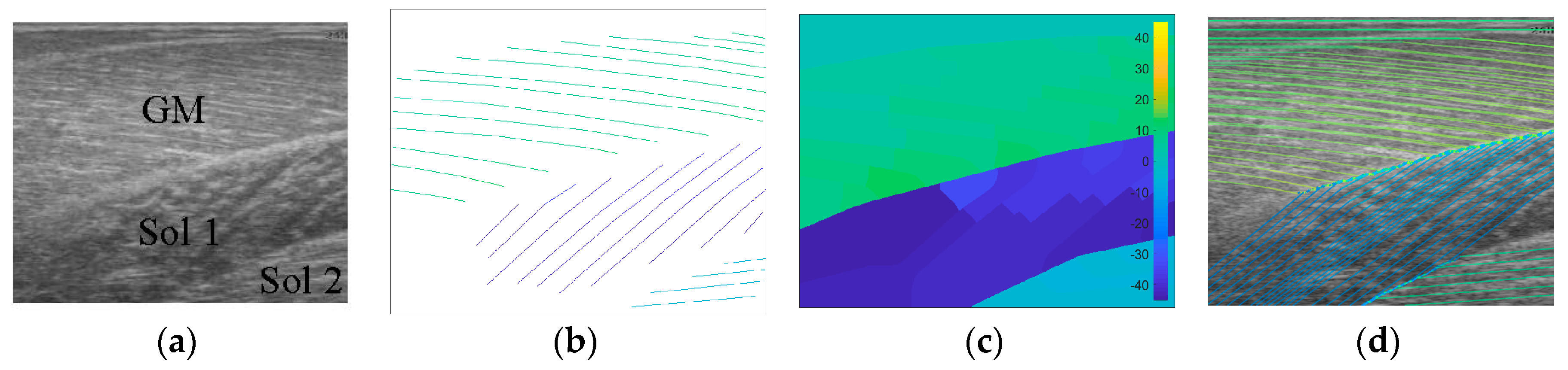
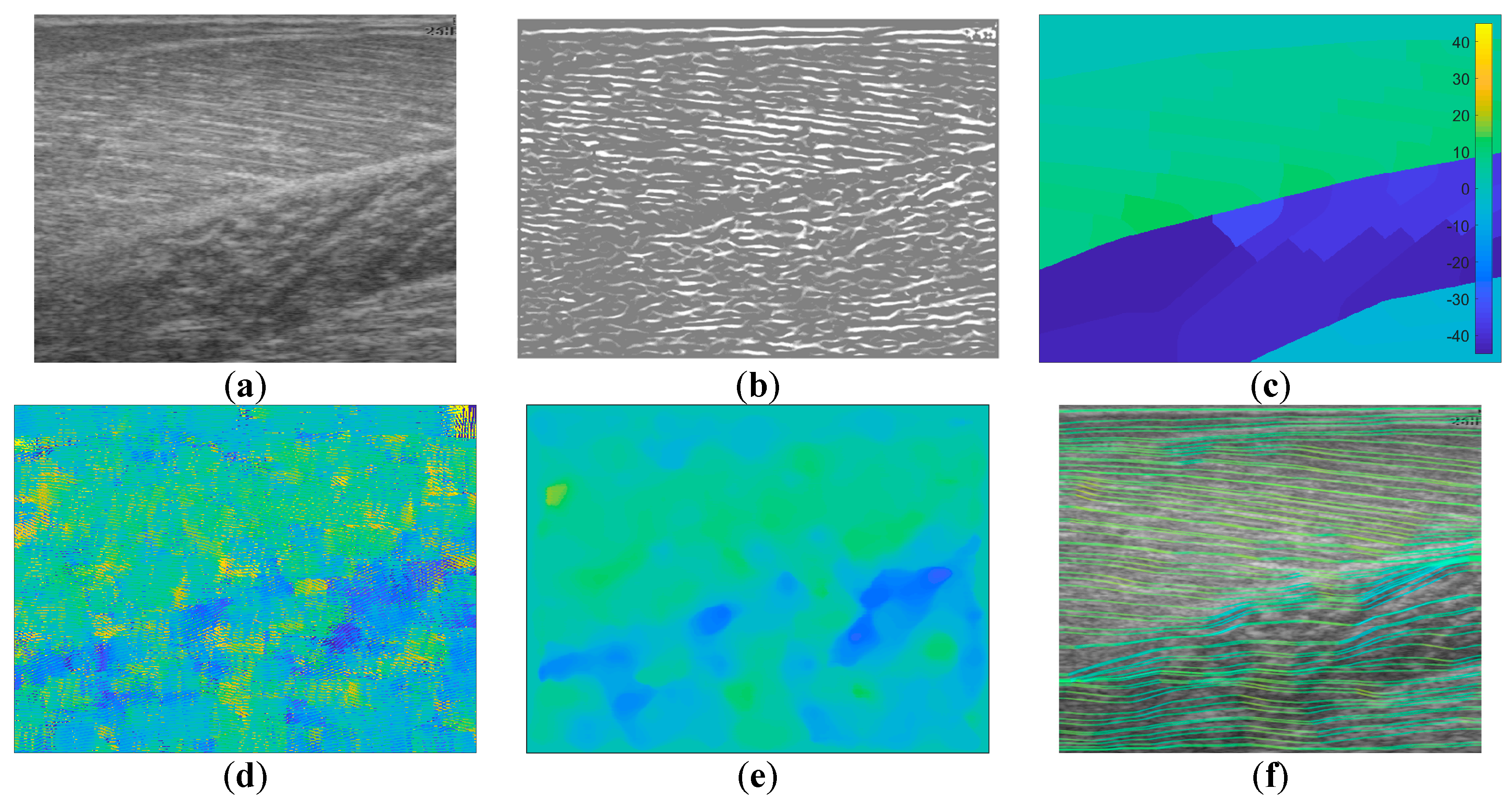
To create labels for each pixel, first a blank image (matrix of zeros with equal dimensions to the ultrasound image) was created. Then, the angles along each of the annotated fibre lines were calculated and for each pixel under the lines the calculated angle was stored. The result was an image of mostly zeroes and a few angled lines, where the value of the non-zero pixels represents the local angle of the line intersecting each pixel. Then, within each muscle/compartment (defined by the experts), nearest neighbour interpolation was used to fill the gaps between lines, followed by nearest neighbour extrapolation to fill the muscle/compartment. Between muscles/compartments, nearest neighbour interpolation was also used to fill the gaps. All other pixels (outside muscle, e.g., skin) were set to zero (see Figure 1). Following, additional data were created to introduce variation in the data/labels and help prevent over-fitting, by randomly (uniform) rotating each image and corresponding labels/angles between −5° and 5°, thus doubling the size dataset to 1008.

2.4. Wavelet Filter Bank Method

The wavelet method was implemented faithful to the original paper [7]. A bank of 180 Gabor wavelet filters was generated spanning 0°–179° in 1° increments using,

$$g\left(x,y\right)=e^{\left(\frac{{\left(x-k-1\right)}^2{\left(y-k-1\right)}^2}{-dk}\right)}\cos \left(\frac{2\pi \left(\left(x-k-1\right)\cos \left(\alpha \right)-\left(y-k-1\right)\sin \left(\alpha \right)\right)}{f}\right)$$

(1)

where k is the half-width of the kernel size (k = 20 pixels = 2.2717 mm), d is a damping term (d = 51.243), α is the orientation and f is the spatial frequency (f = 7). Initially, all parameters were set as originally described in [7] and after a first analysis, some parameters (f and k) were varied (f = 9, f = 11, f = 13, k = f × 3 − 1) to give some scope to the potential of this method on real data. Vessel enhancement was performed using a Matlab version of the Frangi multiscale vessel enhancement filter [31] which can be found here [32]. 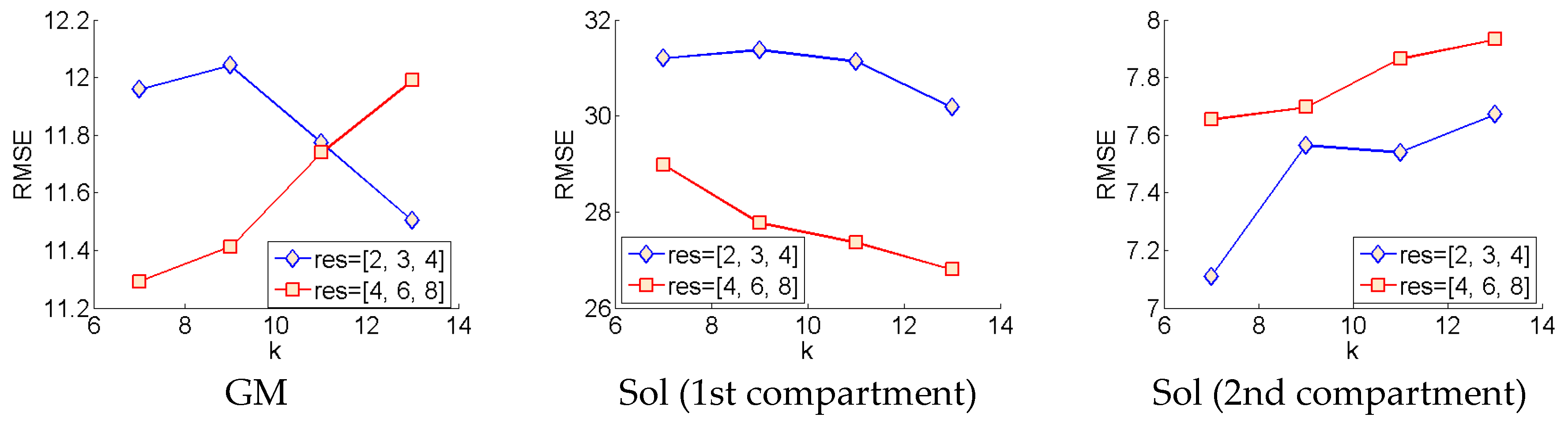Following [7], filtering was performed at 3 sigma scales parameter in the code), 2, 3 and 4. Following a first analysis, a second analysis was done at sigma scales, 4, 6 and 8, for all variants of the Gabor wavelet filters described above.

To analyse an image, the image was filtered with the vessel enhancement filter and then convolved with the entire wavelet filter bank. At each spatial location in the image, we take the α corresponding to the filter with the highest convolution in that location. The result is a map of local orientations (Figure 4). Following [7], the image was then convolved with a 35 × 35 median filter resulting in the final map of local fibre orientations.

2.5. Deconvolution Neural Network Method

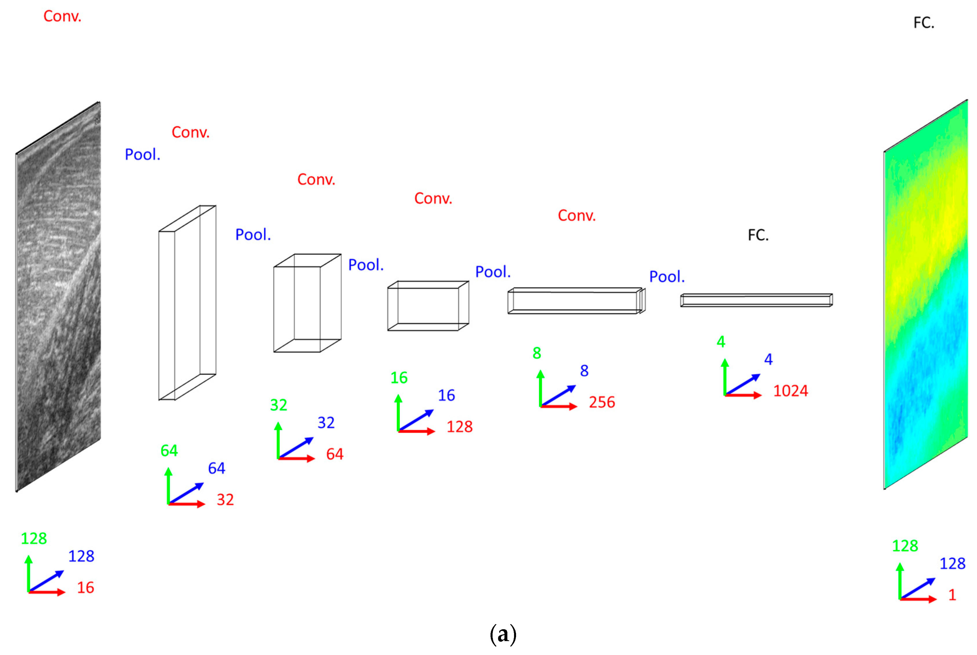
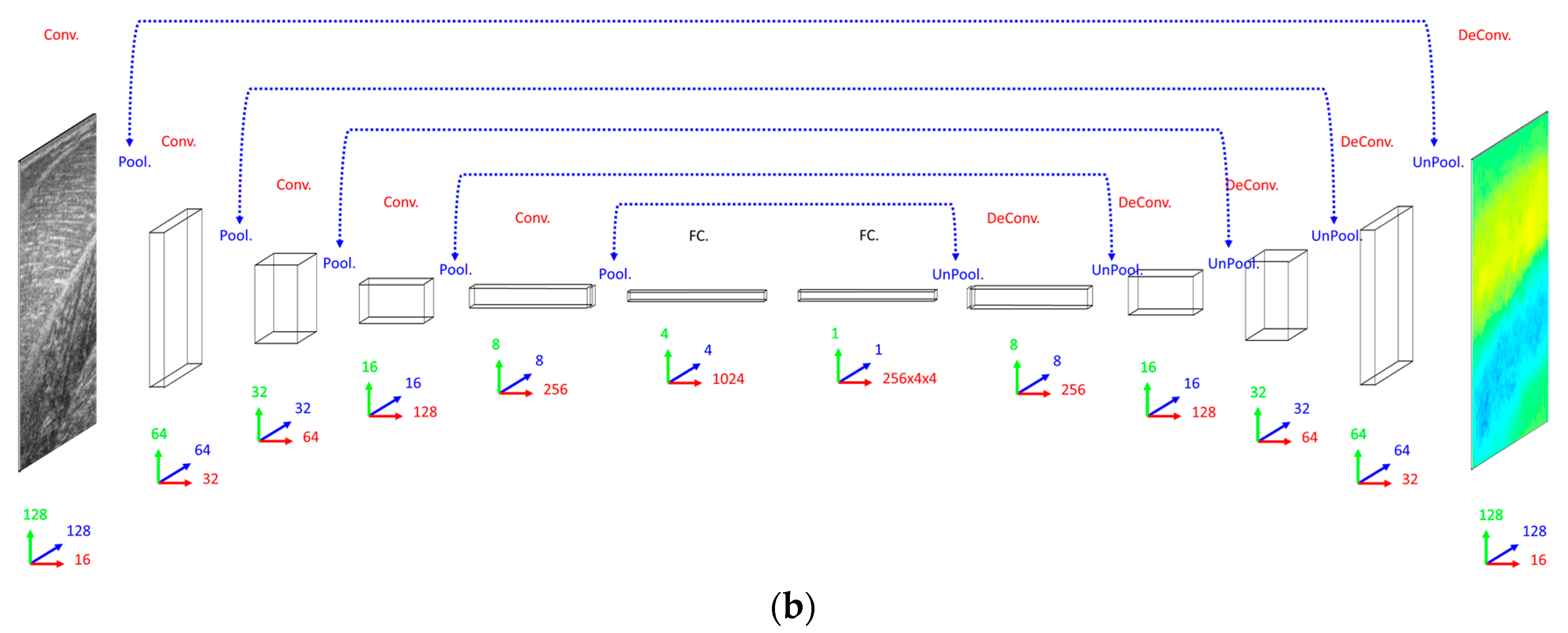
Our primary concern when deciding on a DCNN architecture (number of layer and units per layer) was having a complex enough model to learn the training set. The DCNN implemented 16 convolutional filters in the input layer, with 4 additional convolutional layers, each with double the number of filters in the preceding convolutional layer. Our secondary concern was training time, since we planned to execute an 8-fold cross-validation. Therefore, both input images and labels were down-sampled (bilinear interpolation) to 128 × 128 pixels. Between convolutional layers, the spatial dimensions were down-sampled (max-pooling) by a factor of 2. A dense fully connected layer of 1024 nodes was fully connected to an initial up-sampling (2 × 2 max-un-pooling) layer, followed by a deconvolution layer. An additional 4 up-sampling with deconvolutional layers following, completes the network architecture, with the final layer being a full 128 × 128 resolution regression map. Every layer consisted of rectified linear units (ReLU), with the exception of the final (output) layer, which consisted of linear units (see Figure 2).

2.6. Convolutional and Residual Neural Network Methods

When deciding on a CNN/ResNet architecture we opted for the same convolutional architecture as the DCNN, with the exception that the ResNet had a factor of 5 additional convolutional layers, ensuring that our primary concern was met by performing empirical tests on small fractions of training data. Following our previous work [23], for the ResNet, we multiplied the number of convolutional layers in between max-pooling layers by 5, where every other layer we added identity residual connections. Every other aspect of the CNN and ResNet architecture remained the same as the DCNN with the obvious exception of the output layer, which was a dense fully connected layer of linear regression nodes immediately following the 1024 fully connected nodes, rather than deconvolution and up-sampling layers (see Figure 2).

2.7. Training and Cross-Validation

All networks were trained by minimizing mean square error (MSE) between the labels and the output layer using online stochastic gradient descent (batch size of 1 sample). To optimize and test generalization (estimated real-world performance), leave one person out cross-validation was performed on 2 DCNNs, 2 ResNets and 2 CNNs with different dropout parameter settings (0%, 50%), where dropout was enabled in the fully connected layers only. The weights of the neural networks were initialized using Xavier initialization [33]. To train the CNN, ResNet and DCNN we used learning rates of 5 × 10⁻⁶, 2.5 × 10⁻⁶ and 2.5 × 10⁻², respectively. Weight gradient momentum of 9.5 × 10⁻¹ was applied to all networks, which were trained for 100 full batch iterations using stochastic online gradient descent (minibatch = 1). All learning parameters were chosen empirically on a small fraction of the training data. The neural networks were trained 8 distinct times (one for each person), each time reinitializing the networks and leaving a different person out for testing and randomly splitting the remaining data (7 people) into validation and training sets (50% split). Prior to training, the pixels of the input images were normalized over the training (otherwise they were not processed in any way before analysis) set to zero mean and unit variance and pixels of the output images were divided by a constant (45) so that most of the pixels (angles) fell between −1 and +1. Validation and test errors were observed periodically and the test error observed at the lowest validation error (early stopping method) gave results for the validation set and the test set (estimated real-world generalization error). Test results for all held-out participants were combined to reveal the performance of the optimal CNN, ResNet and DCNN.

3. Results

Following model optimization of the wavelet and DCNN methods, both methods were compared against the ground truth labels using a range of error measures, thus making the work accessible and comparable to others. In Section 3.1 and Section 3.2 results are presented respectively for the wavelet method and the DCNN method. With respect to data ranges, within the GM muscle, the maximum range of angles within a single muscle region was 34.84°, whereas the maximum range of angles over all participants was 76.58°. Within the Sol muscle (compartment 1), the maximum range of angles within a single muscle region was 35.02°, whereas the maximum range of angles over all participants was 64.92°. Within the Sol muscle (compartment 2), the maximum range of angles within a single muscle region was 65.15°, whereas the maximum range of angles over all participants was 79.05°.

3.1. Wavelet Method

The wavelet method was evaluated using the optimal parameters (within the range of parameters investigated) for each muscle/compartment, separately. To find the optimal parameters within each muscle, the local orientation over each pixel identified by the wavelet method was compared to each pixel of the ground truth by root mean square error (RMSE) (see Figure 3). Within the parameters we investigated, for the GM muscle, smaller wavelet filters resulted in smaller RMSE for the higher-resolution Frangi filter (res = [4,6,8]), conversely larger wavelet filters result in smaller RMSE for the lower-resolution Frangi filter. Within the parameters we investigated, the first compartment of the Sol muscle yields best results with the higher-resolution Frangi filter and larger wavelet filters. Conversely, within the parameters we investigated, the second compartment of the Sol muscle yields best results for smaller wavelet filters and lower-resolution Frangi filter. The models with the lowest RMSE were compared to ground truth using mean difference (MD) and mean absolute error (MAE), to be compared with the DCNN method (Section 3.2).

For the optimal models within each muscle/compartment, the deviations of predicted local fibre orientations from ground truth were much too high to be useful in any real context, particularly in the Sol (compartment 1) muscle, which reports an optimal RMSE of over 26° (see Figure 3). Discrepancies were much lower in the GM and Sol (compartment 2) muscles at 11.3° and 7.1°, respectively. Visual comparisons were also made by comparing the wavelet analysis, presented as a heat-map, to the ground truth, also presented as a heat-map (see Figure 4). Visual comparison revealed quite sporadic agreement between wavelet predictions and ground truth. Visual comparison also revealed that any agreement between wavelet predictions and ground truth was not only heavily dependent on the presence of well-defined muscle fibre tracts, but also on the ability of the Frangi filter to extract those features (Figure 4).

3.2. DCNN Method

The deep learning methods were evaluated using the optimal models as identified by cross-validation (see Figure 5). The output heat-map from the optimal neural networks were compared to the ground truth using mean difference (MD) and mean absolute error (MAE), to be compared with the wavelet method (see

Table 1. Table of results per muscle/compartment. This table shows results computed by comparing predictions of each method, over all pixels (128 × 128 = 16,384), to the ground truth.

Muscle	Error Measure	Namburete, et al. [7]	CNN [23]	ResNet [23]	DCNN (Proposed)
GM	MD 1	7.57° ± 8.37°	6.67° ± 10.21°	6.75° ± 11.06°	3.27° ± 10.10°
	MAE 2	8.23° ± 7.72°	8.08° ± 9.13°	8.68° ± 9.61°	6.87° ± 8.09°
	RMSE 3	11.29°	12.19°	12.96°	10.62°
Sol 1	MD 1	−22.84° ± 14.01°	−10.18° ± 9.37°	−11.28° ± 9.63°	−5.67° ± 10.59°
	MAE 2	23.09° ± 13.61°	11.19° ± 8.14°	12.06° ± 8.63°	9.01° ± 7.94°
	RMSE 3	26.80°	13.84°	14.83°	12.01°
Sol 2	MD 1	1.61° ± 6.92°	6.07° ± 8.76°	6.08° ± 7.87°	6.17° ± 9.57°
	MAE 2	5.03° ± 5.01°	8.76° ± 8.55°	7.86° ± 6.09°	8.94° ± 7.05°
	RMSE 3	7.11°	10.66°	9.95°	11.39°

¹ Mean difference = $\frac{1}{n}{\displaystyle \sum }{x}_i-y_i$. ² Mean absolute error = $\frac{1}{n}{\displaystyle \sum }\left|x_i-y_i\right|$. ³ Root mean square error = $\sqrt{\frac{1}{n}{\displaystyle \sum }{\left(x_i-y_i\right)}^2}$.

). Visual comparisons were also made by comparing the neural networks’ predicted heat-maps to the ground truth heat-maps (see Figure 6). The most immediate result of visual comparisons was the ability of the DCNN to “colour-code” the correct regions; the GM and Sol (compartment 1) muscles typically present with opposing fibre orientations, with negative angles in the Sol muscle and positive angles in the GM muscle. In almost all images the DCNN was able to identify the Sol and GM muscles by predicting correct signs of the angles for each compartment. This was broadly true for entire muscle regions, even where there were no visibly identifiable fibres (see Figure 6). The CNN and ResNet models showed more difficulty in identifying regions and features of this drawback are visible in the graphics presented in Figure 6; horizontal striping patterns can be seen in the heatmaps, indicating the networks learned templates for each muscle position, which implies that if it has not seen an example muscle of a certain shape/thickness before, it will not generalize to it—whereas the DCNN has a lot of built in position invariance due to deconvolution and up-sampling via the max pooling argmax.

Further to quantitative (Table 1) and visual (Figure 6) analysis, we present additional time-series data for a representative test participant (Figure 7). The DCNN (and the other three method) estimates regional fibre orientation independently for each frame. Figure 7 shows estimates of sequential frames for a representative test participant. The temporal variation in fibre orientation represents the changes during muscle contraction very well in GM, but less well for the Sol 1 and 2 compartments. The continuity of the fibre angle between frames demonstrates the potential usefulness of this method to estimate time-varying behaviour, in real-time, without the accumulation of error (drift) that results from inter-frame tracking methods.

4. Discussion

In this paper, we presented an investigation into the feasibility of using deep learning methods for developing arbitrary full spatial resolution regression analysis of B-mode ultrasound images of human skeletal muscle. Four different methods were compared, feature engineering, convolutional neural networks (CNN), residual convolutional neural networks (ResNet) and deconvolutional neural networks (DCNN), for estimating full spatial resolution muscle fibre orientation in multiple deep muscle layers, directly from B-mode ultrasound images. The efficacy of this work has shown that the deep learning methods are feasible and particular deep learning methods, DCNNs, work best due to the spatial organization of the output regression map, which intelligently reduces the number of free parameters, preventing over-fitting. The previous established approach, wavelets, lacked accuracy and is limited in application, due to an inherent inability to ignore spurious fibre structures and the requirement for accurate segmentation to apply different wavelet frequencies within different regions.

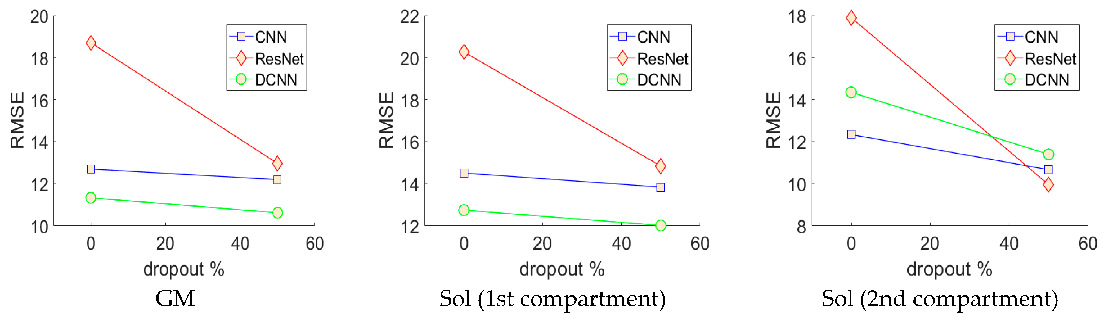
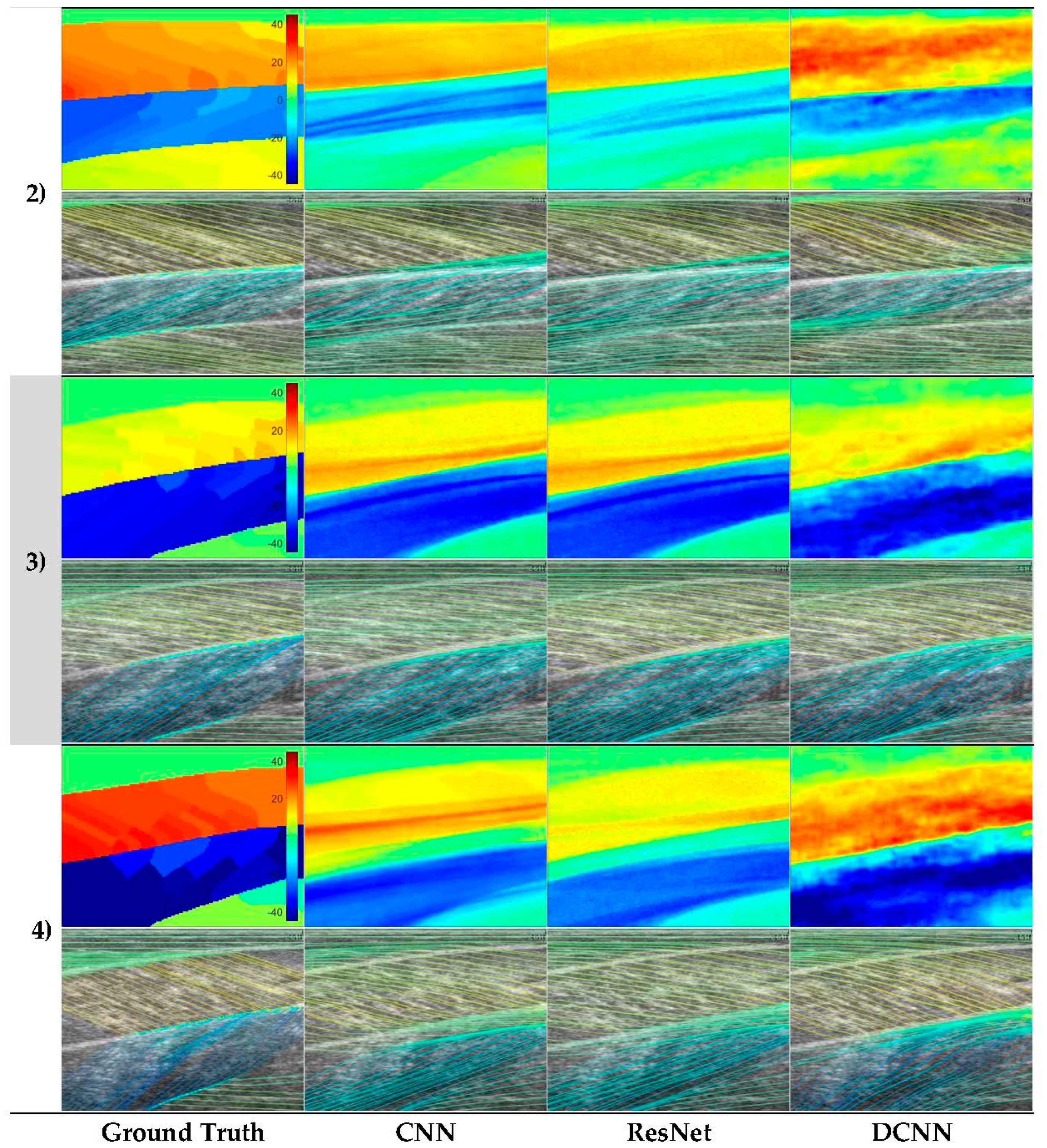
Analysis of each deep learning method revealed the strength of the approach and moreover, the strength of the DCNN approach. Both CNN and ResNets outperformed the wavelet approach (see Table 1) in GM and Sol 1 muscles. However, the DCNN outperformed the CNN and ResNet markedly. Our interpretation is that the CNN/ResNet methods learned templates of the fibre orientation maps based on muscle dimensions in the training set, resulting in comparatively (to DCNN) poor localization of the muscle regions. Artefacts of this can be seen in Figure 6, where the heatmaps of CNN/ResNet present with horizontal striping patterns, which are very likely different muscle boundary templates which have been combined to make the new orientation map. The DCNN showed the remarkable ability localize muscle regions and roughly match the colour intensity of the heatmap, which resulted in accurate and visibly pleasing fibre traces (see Figure 6 and Figure 7). Figure 6 shows examples of CNN/ResNet methods performing better than DCNN in specific regions (e.g., rows 3–4 in the Sol 1 region), which can also be explained with the templates argument; i.e., where the test image did not match the templates well, performance was weaker and where the test image matched the templates well, performance was stronger.

In contrast to the deep learning methods, Figure 1 shows a representative output from the wavelet method, which appeared to perform well on the GM muscle and not on the other 2 muscles/compartments. In the Sol 1 muscle, where fibres are visible, some the wavelet analysis produces a very localized response which is roughly correct, but unfortunately this type of performance was common over the data set, resulting in very poor results in Table 1. However, the wavelet method did show comparable performance to the DCNN in the GM muscle, which is certainly because of the texturally well-defined fibre structures in this region. Thee deep muscles in this muscle group often present differently, due to differences in architecture and other arguably more minor reasons like attenuation of the ultrasound beams, reflections, image artefacts and signal dropout. For this reason, results of all four methods are adversely affected in the deeper muscles. In the deepest compartment, defying the logical argument we just presented, the wavelet method produced notably the best performance. It is worth noting that the angles in that muscle region, annotated by the expert, were very commonly 0°, or some positive or negative number close to 0°. The wavelet method used local neighbourhood (35 × 35) median averaging of angles in a range of (–90:90). Therefore, our interpretation is that if we take the median of a set of random positive and negative angles, we would “guess” fibre orientations, close to the ground truth. Although, this could be a genuine result, the other issues with the wavelet approach are more devastating, even when compared to the CNN/ResNet approaches and particularly when compared to the DCNN.

The results presented in Table 1 for the deep learning methods represent a truly generalized and thoroughly tested expectation of real-world performance. Test results were acquired by leave one participant out testing for all 8 participants (8-fold cross-validation; see Figure 5), which is the harshest possible test of performance and generalization for this approach, requiring intensive training of 48 neural networks, which took less than a week on the latest GPU compute technology (GTX 1080 Ti). Depending upon the problem, handcrafting features such as Gabor wavelets can be much more time consuming and must be tailored to solve specific problems. What is more, the results we present in Table 1 on the wavelet method, represent the optimal performance given accurate segmentation, since different wavelet frequencies and image filters were applied to different regions of the image—this would obviously not be possible without accurate and presumably automatic segmentation.

The implications of the efficacy of DCNNs for regression analysis with respect to skeletal muscle ultrasound, is in the application to other, high-impact research problems. The ability to produce a full resolution map of tissue strain, for example, would very likely and very positively impact the way musculoskeletal healthcare was delivered. Currently, elastography is the only non-invasive method for estimating strain within specific skeletal muscles [35] and it has serious theoretical flaws; elastography currently has a maximum temporal resolution of 1 Hz and due to the anisotropy of skeletal muscle, the theory is only empirically validated for skeletal muscle when the ultrasound probe is parallel to the fibres [36]. DCNNs can be used to estimate full resolution motion maps [26]. Such technology would allow localization of muscle twitches, which has applications in the diagnosis and monitoring of motor neurone disease [1,2]. Analysis of local strain would also provide a non-invasive technology for diagnosis, targeting and monitoring treatment of conditions such as dystonia (a neurological condition causing painful muscle cramping/spasming). For example, diagnosis of cervical dystonia is currently done by needle electromyography (EMG), which is highly invasive, limiting/preventing treatment and diagnosis of deeper muscles (near the spine in the back and neck). We note that these applications are beyond the scope of the wavelet approach, whereas the DCNN method opens this entire domain for investigation, since we demonstrate feasibility in the application, even when constrained by small data sets. Our DCNN implementation can process an image (copy image to GPU, feedforward through the network and copy predicted fibre orientation map from GPU) at approximately 165 images per second, which is applicable to real-time operation within a clinic, lab or hospital.

5. Conclusions

The novel contribution of this paper is in the application of neural networks to skeletal muscle ultrasound for full spatial regression analysis of muscle fibre orientation. We provided the first comprehensive analysis of an existing and a novel computational method for estimating full regional fibre orientation from ultrasound images of human skeletal muscle. We have proposed a novel application of deep learning to a long-standing and challenging problem and demonstrated state of the art results. We present analyses in a form which is comparable to any future developments and we also publish our ultrasound and ground truth data to support this end (see Supplementary Material for Matlab data files). The application of DCNNs to this problem has opened new potential to hi-resolution analysis of skeletal muscle, from prediction of strain and motion maps to segmentation of muscles and other structures of interest. This paper provides further evidence that deep learning methods can surpass state of the art performance, even when there is not an abundance of labelled data available, just by organizing the architecture (deconvolutions) of the network. With additional data, we propose that this project could easily be extended successfully and this preliminary muscle analysis step could very likely form part of a skeletal muscle analysis system which accurately predicts the passive and active muscle forces non-invasively directly from single ultrasound images and sequences. Such a contribution could enable early diagnoses of diseases such as MND and would enable personalized musculoskeletal medical diagnosis, monitoring, treatment targeting and care, for disease such as stroke, back pain, neck pain, dystonia and myositis.

References

1. Harding, P.J.; Loram, I.D.; Combes, N.; Hodson-Tole, E.F. Ultrasound-based detection of fasciculations in healthy and diseased muscles. IEEE Trans. Biomed. Eng. 2016, 63, 512–518. [Google Scholar] [CrossRef] [PubMed]
2. Harding, P.J.; Hodson-Tole, E.F.; Cunningham, R.; Loram, I.; Costen, N. Automated detection of skeletal muscle twitches from B-mode ultrasound images: An application to motor neuron disease. In Proceedings of the 21st International Conference on Pattern Recognition (ICPR), Tsukuba, Japan, 11–15 November 2012; pp. 2630–2633. [Google Scholar]
3. Loram, I.D.; Bate, B.; Harding, P.; Cunningham, R.; Loram, A. Proactive selective inhibition targeted at the neck muscles: This proximal constraint facilitates learning and regulates global control. IEEE Trans. Neural Syst. Rehabil. Eng. 2017, 25, 357–369. [Google Scholar] [CrossRef] [PubMed]
4. Loram, I.; Maganaris, C.; Lakie, M. Use of ultrasound to make noninvasive in vivo measurement of continuous changes in human muscle contractile length. J. Appl. Physiol. 2006, 100, 1311–1323. [Google Scholar] [CrossRef] [PubMed]
5. Zhou, G.Q.; Chan, P.; Zheng, Y.P. Automatic measurement of pennation angle and fascicle length of gastrocnemius muscles using real-time ultrasound imaging. Ultrasonics 2015, 57, 72–83. [Google Scholar] [CrossRef] [PubMed]
6. Rana, M.; Hamarneh, G.; Wakeling, J.M. Automated tracking of muscle fascicle orientation in B-mode ultrasound images. J. Biomech. 2009, 42, 2068–2073. [Google Scholar] [CrossRef] [PubMed]
7. Namburete, A.I.L.; Rana, M.; Wakeling, J.M. Computational methods for quantifying in vivo muscle fascicle curvature from ultrasound images. J. Biomech. 2011, 44, 2538–2543. [Google Scholar] [CrossRef] [PubMed]
8. Chen, X.; Li, Q.; Qi, S.; Zhang, H.; Chen, S.; Wang, T. Continuous fascicle orientation measurement of medial gastrocnemius muscle in ultrasonography using frequency domain Radon transform. Biomed. Signal Process. Control 2015, 20, 117–124. [Google Scholar] [CrossRef]
9. Darby, J.; Li, B.; Costen, N.; Loram, I.; Hodson-Tole, E. Estimating skeletal muscle fascicle curvature from B-mode ultrasound image sequences. IEEE Trans. Biomed. Eng. 2013, 60, 1935–1945. [Google Scholar] [CrossRef] [PubMed] [Green Version]
10. Herbert, R.D.; Gandevia, S.C.; Herbert, R.D. Changes in pennation with joint angle and muscle torque: In vivo measurements in human brachialis muscle. J. Physiol. 1995, 484, 523–532. [Google Scholar] [CrossRef] [PubMed]
11. Narici, M.V.; Binzoni, T.; Hiltbrand, E.; Fasel, J.; Terrier, F.; Cerretelli, P. In vivo human gastrocnemius architecture with changing joint angle at rest and during graded isometric contraction. J. Physiol. 1996, 496, 287–297. [Google Scholar] [CrossRef] [PubMed]
12. Lieber, R.L.; Fridén, J. Functional and clinical significance of skeletal muscle architecture. Muscle Nerve 2000, 23, 1647–1666. [Google Scholar] [CrossRef]
13. Zhou, Y.; Li, J.-Z.; Zhou, G.; Zheng, Y.-P. Dynamic measurement of pennation angle of gastrocnemius muscles during contractions based on ultrasound imaging. Biomed. Eng. Online 2012, 11, 63. [Google Scholar] [CrossRef] [PubMed]
14. Zhou, G.Q.; Zheng, Y.P. Automatic fascicle length estimation on muscle ultrasound images with an orientation-sensitive segmentation. IEEE Trans. Biomed. Eng. 2015, 62, 2828–2836. [Google Scholar] [CrossRef] [PubMed]
15. Chen, F. Hand gesture recognition using a real-time tracking method and hidden Markov models. Image Vis. Comput. 2003, 21, 745–758. [Google Scholar] [CrossRef]
16. Zhou, Y.; Zheng, Y.P. Estimation of muscle fiber orientation in ultrasound images using Revoting Hough Transform (RVHT). Ultrasound Med. Biol. 2008, 34, 1474–1481. [Google Scholar] [CrossRef] [PubMed]
17. Stark, H.; Schilling, N. A novel method of studying fascicle architecture in relaxed and contracted muscles. J. Biomech. 2010, 43, 2897–2903. [Google Scholar] [CrossRef] [PubMed]
18. Krizhevsky, A.; Sutskever, I.; Hinton, G.E. ImageNet Classification with Deep Convolutional Neural Networks. In Proceedings of the 25th International Conference on Neural Information Processing Systems, Lake Tahoe, NV, USA, 3–6 December 2012; pp. 1–9. [Google Scholar]
19. He, K.; Zhang, X.; Ren, S.; Sun, J. Deep Residual Learning for Image Recognition. In Proceedings of the 2016 IEEE Conference on Computer Vision and Pattern Recognition (CVPR), Las Vegas, NV, USA, 27–30 June 2016; pp. 770–778. [Google Scholar]
20. Hinton, G. Dropout : A Simple Way to Prevent Neural Networks from Overfitting. J. Mach. Learn. Res. 2014, 15, 1929–1958. [Google Scholar]
21. Nair, V.; Hinton, G.E. Rectified Linear Units Improve Restricted Boltzmann Machines. In Proceedings of the 27th International Conference on International Conference on Machine Learning, Haifa, Israel, 21–24 June 2010; pp. 807–814. [Google Scholar]
22. Jackel, L.D.L.; Boser, B.; Denker, J.S.; Henderson, D.; Howard, R.E.; Hubbard, W.; Le Cun, B.; Denker, J.; Henderson, D. Handwritten Digit Recognition with a Back-Propagation Network. In Advances in Neural Information Processing Systems 2; Morgan Kaufmann Publishers Inc.: San Francisco, CA, USA, 1990; pp. 396–404. [Google Scholar]
23. Cunningham, R.J.; Harding, P.J.; Loram, I.D. Deep residual networks for quantification of muscle fiber orientation and curvature from ultrasound. In Medical Image Understanding and Analysis; Springer: Cham, Switzerland, 2017; pp. 63–73. [Google Scholar]
24. Cunningham, R.; Harding, P.; Loram, I. Real-Time Ultrasound Segmentation, Analysis and Visualization of Deep Cervical Muscle Structure. Trans. Med. Imaging 2017, 36, 653–665. [Google Scholar] [CrossRef] [PubMed]
25. Pfister, T.; Charles, J.; Zisserman, A. Flowing convnets for human pose estimation in videos. In Proceedings of the IEEE International Conference on Computer Vision, Santiago, Chile, 7–13 December 2015; pp. 1913–1921. [Google Scholar]
26. Fischer, P.; Dosovitskiy, A.; Ilg, E.; Häusser, P.; Hazırbaş, C.; Golkov, V.; van der Smagt, P.; Cremers, D.; Brox, T. FlowNet: Learning Optical Flow with Convolutional Networks. In Proceedings of the 2015 IEEE International Conference on Computer Vision (ICCV), Santiago, Chile, 7–13 December 2015; p. 8. [Google Scholar]
27. Payer, C.; Štern, D.; Bischof, H.; Urschler, M. Regressing heatmaps for multiple landmark localization using CNNs. In Lecture Notes in Computer Science (Including Subseries Lecture Notes in Artificial Intelligence and Lecture Notes in Bioinformatics); Springer: Cham, Switzerland, 2016; Volume 9901 LNCS, pp. 230–238. [Google Scholar]
28. Noh, H.; Hong, S.; Han, B. Learning deconvolution network for semantic segmentation. In Proceedings of the IEEE International Conference on Computer Vision, Washington, DC, USA, 7–13 December 2015; Volume 11–18, pp. 1520–1528. [Google Scholar]
29. Ronneberger, O.; Fischer, P.; Brox, T. U-Net: Convolutional Networks for Biomedical Image Segmentation. In Medical Image Computing and Computer-Assisted Intervention (MICCAI); Springer LNCS: Berlin, Germany, 2015; Volume 9351, pp. 234–241. [Google Scholar]
30. Zeiler, M.D.; Fergus, R. Visualizing and Understanding Convolutional Networks. arXiv:1311.2901v3 [cs.CV] 28 November 2013. Comput. Vis. Pattern Recognit. 2014, 8689, 818–833. [Google Scholar]
31. Frangi, A.F.; Niessen, W.J.; Vincken, K.L.; Viergever, M.A. Multiscale vessel enhancement filtering. In Medical Image Computing and Computer-Assisted Intervention—MICCAI’98. MICCAI 1998. Lecture Notes in Computer Science; Springer: Berlin/Heidelberg, Germany, 1998; Volume 1496, pp. 130–137. [Google Scholar]
32. Kroon, D.J. Hessian based Frangi Vesselness filter. MATLAB Central/File Exchange. 2010. Available online: https://uk.mathworks.com/matlabcentral/fileexchange/24409-hessian-based-frangi-vesselness-filter (accessed on 1 November 2017).
33. Glorot, X.; Bengio, Y. Understanding the difficulty of training deep feedforward neural networks. In Proceedings of the 13th International Conference on Artificial Intelligence and Statistics (AISTATS), Sardinia, Italy, 13–15 May 2010; Volume 9, pp. 249–256. [Google Scholar]
34. Darby, J.; Hodson-Tole, E.F.; Costen, N.; Loram, I.D. Automated regional analysis of B-mode ultrasound images of skeletal muscle movement. J. Appl. Physiol. 2012, 112, 313–327. [Google Scholar] [CrossRef] [PubMed]
35. Hug, F.; Tucker, K.; Gennisson, J.L.; Tanter, M.; Nordez, A. Elastography for Muscle Biomechanics: Toward the Estimation of Individual Muscle Force. Exerc. Sport Sci. Rev. 2015, 43, 125–133. [Google Scholar] [CrossRef] [PubMed]
36. Eby, S.F.; Song, P.; Chen, S.; Chen, Q.; Greenleaf, J.F.; An, K.N. Validation of shear wave elastography in skeletal muscle. J. Biomech. 2013, 46, 2381–2387. [Google Scholar] [CrossRef] [PubMed]
Figure 1. Image annotation. (a) shows the raw ultrasound image and 3 muscles/compartments (Grey model (GM), Sol 1 and Sol 2), (b) shows expert annotated line traces of visible fibre paths, (c) shows nearest neighbour region filling of annotated fibre paths within annotated muscles/compartments, (d) shows line traces over the filled regions.
Jimaging 04 00029 g001
Figure 2. Network schemas. (a) Top: Convolutional Neural Network (CNN) with 5 convolutional layers (Conv.), 5 max-pooling layers (Pool.) and 2 fully connected layers (FC.). Bottom: Residual Neural Network (ResNet) with 25 convolutional layers (Conv.), 5 max-pooling layers (Pool.) and 2 fully connected layers (FC.), where residual (identity) connections are shown (dashed blue lines). (b) Deconvolutional Neural Network (DCNN) with 5 convolutional layers (Conv.), 5 max-pooling layers (Pool.), 5 deconvolutional layers (DeConv.), 5 max-un-pooling layers (UnPool.) and 2 fully connected layers (FC.), where dashed blue lines indicate argmax link between un-pooling and pooling layers. Network size/complexity and runtime (forward pass, average over 1000 runs) is indicated below respective schematics. In all graphics, blue, green and red arrows/numbers respectively represent horizontal (pixels), vertical (pixels) and feature (nodes) dimensions per layer.
Jimaging 04 00029 g002aJimaging 04 00029 g002b
Figure 3. Wavelet parameter tuning. This graphic depicts how the error changes with respect to the parameters of the Frangi filter (res) and the Gabor wavelet filters (k).
Jimaging 04 00029 g003
Figure 4. Representative wavelet visual result. (a) shows the raw image, (b) shows the vessel-enhanced image (contrast-enhanced for clarity), (c) shows the ground truth, (d) shows the result of Gabor wavelet convolution with (b,e) shows the result of a (35 × 35) median filter applied to (d,f) shows line traces of (e). It is clear, when comparing (e) to (c), that the heatmaps partial match within the GM region, but almost not at all in the Sol region. The line trace visually confirms that the fibre traces are roughly aligned with the visible fibres in the raw image in the GM muscle and the second compartment of the Sol muscle only. The heatmap (d,e) does not consistently represent the segmentation of muscle compartments shown by the ground truth.
Jimaging 04 00029 g004
Figure 5. Neural network cross-validation. This graphic depicts how the error changes with respect to the percentage of dropout enabled in the fully connected layers of the CNN, ResNet and DCNN. These results show that dropout lowered RMSE, with 50% dropout enabled, revealing the optimal model for each architecture. Notice the ResNet without dropout enabled suffers from severe over-fitting.
Jimaging 04 00029 g005
Figure 6. Representative neural network predictions. Rows 1–4 show four respective test participants in the dataset. In each row, the top image shows a fibre orientation heatmap and the bottom image shows a line trace representation of the heatmap, overlaid on the ultrasound image. Columns show respectively, ground.
Jimaging 04 00029 g006aJimaging 04 00029 g006b
Figure 7. DCNN fibre orientation time-series. Left: shows fibre traces predicted by the DCNN at time points corresponding to a maximum voluntary contraction beginning at 0 s and ending at 2.2 s, where the time point is indicated below each graphic. Notice the sharp increase in angles of the fibres in the GM muscle as the contraction develops from top to bottom graphic (0.6–1.8 s). Right: shows, for a representative participant, average fibre angles, predicted by the DCNN over a maximum voluntary contraction, for each muscle (solid blue line), plus and minus 1 standard deviation (dashed blue line) and average fibre angles of the ground truth for the same contraction (solid green lines), plus and minus 1 standard deviation (dashed green lines). For GM, agreement is high until the latter part of the contraction, whereas for Sol (1 and 2), estimation appears to have failed, although compartment 1 does show an increased standard deviation which tracks the increase in angle, which may indicate curvature in the model and not in the labels. We note that this approach is superior to feature tracking [34] because there is no possibility of tracking drift with the proposed method. Please see supplementary material for a video of the fibre line traces in this figure.
Jimaging 04 00029 g007