Efficient Query Specific DTW Distance for Document Retrieval with Unlimited Vocabulary


1
Center for Visual Information Technology, IIIT Hyderabad, Hyderabad 500 032, India
2
CSE Department, Stony Brook University, Stony Brook, NY 11794, USA
3
Department of Computer Science and Engineering, IIT Jodhpur, Jodhpur 342037, India
*
Author to whom correspondence should be addressed.
J. Imaging 2018, 4(2), 37; https://0-doi-org.brum.beds.ac.uk/10.3390/jimaging4020037
Submission received: 31 October 2017
/
Revised: 27 January 2018
/
Accepted: 2 February 2018
/
Published: 8 February 2018
(This article belongs to the Special Issue Document Image Processing)
Abstract
:In this paper, we improve the performance of the recently proposed Direct Query Classifier (dqc). The (dqc) is a classifier based retrieval method and in general, such methods have been shown to be superior to the OCR-based solutions for performing retrieval in many practical document image datasets. In (dqc), the classifiers are trained for a set of frequent queries and seamlessly extended for the rare and arbitrary queries. This extends the classifier based retrieval paradigm to an unlimited number of classes (words) present in a language. The (dqc) requires indexing cut-portions (n-grams) of the word image and dtw distance has been used for indexing. However, dtw is computationally slow and therefore limits the performance of the (dqc). We introduce query specific dtw distance, which enables effective computation of global principal alignments for novel queries. Since the proposed query specific dtw distance is a linear approximation of the dtw distance, it enhances the performance of the (dqc). Unlike previous approaches, the proposed query specific dtw distance uses both the class mean vectors and the query information for computing the global principal alignments for the query. Since the proposed method computes the global principal alignments using n-grams, it works well for both frequent and rare queries. We also use query expansion (qe) to further improve the performance of our query specific dtw. This also allows us to seamlessly adapt our solution to new fonts, styles and collections. We have demonstrated the utility of the proposed technique over 3 different datasets. The proposed query specific dtw performs well compared to the previous dtw approximations.
1. Introduction
Retrieving relevant documents (pages, paragraphs or words) is a critical component in information retrieval solutions associated with digital libraries. The problem has been looked at in two settings: recognition based [1,2] like ocr and recognition free [3,4]. Most of the present day digital libraries use Optical Character Recognizers (ocr) for the recognition of digitized documents and thereafter employ a text based solution for the information retrieval. Though ocrs have become the de facto preprocessing for the retrieval, they are realized as insufficient for degraded books [5], incompatible for older print styles [6], unavailable for specialized scripts [7] and very hard for handwritten documents [8]. Even for printed books, commercial ocrs may provide highly unacceptable results in practice. The best commercial ocrs can only give word accuracy of 90% on printed books [4] in modern digital libraries. This means that every 10th word in a book is not searchable. Recall of retrieval systems built on such erroneous text is thus limited. Recognition free approaches have gained interest in recent years. Word spotting [3] is a promising method for recognition free retrieval. In this method, word images are represented using different features (e.g., Profiles, sift-bow), and the features are compared with the help of appropriate distance measures (Euclidean, Earth Movers [9], dtw [10]). Word spotting has the advantage that it does not require prior learning due to its appearance-based matching. These techniques have been popularly used in document image retrieval.
Konidaris et al. [5] retrieve words from a large collection of printed historical documents. A search keyword typed by the user is converted into a synthetic word image which is used as a query image. Word matching is based on computing the distance metric between the query feature and all the features in the database. Here the features are calculated using the density of the character pixels and the area that is formed from the projections of the upper and lower profile of the word. The ranked results are further improved by relevance feedback. Sankar and Jawahar [7] have suggested a framework of probabilistic reverse annotation for annotating a large collection of images. Word images were segmented from 500 Telugu books. Matching of the word images is done using the dtw approach [11]. Hierarchical agglomerative clustering was used to cluster the word images. Exemplars for the keywords are generated by rendering the word to form a keyword-image. Annotation involved identifying the closest word cluster to each keyword cluster. This involves estimating the probability that each cluster belongs to the keyword. Yalniz and Manmatha [4] have applied word spotting to scanned English and Telugu books. They are able to handle noise in the document text by the use of sift features extracted on salient corner points. Rath and Manmatha [11] used projection profile and word profile features in a dtw based matching technique.
Recognition free retrieval was attempted in the past for printed as well as handwritten document collections [4,7,12,13]. Since most of these methods were designed for smaller collections (few handwritten documents as in [12]), computational time was not a major concern. Methods that extended this to a larger collection [14,15,16] used mostly (approximate) nearest neighbor retrieval. For searching complex objects in large databases, svms have emerged as the most popular and accurate solution in the recent past [12]. For linear svms, both training and testing have become very fast with the introduction of efficient algorithms and excellent implementations [17]. However, there are two fundamental challenges in using a classifier based solution for word retrieval (i) A classifier needs a good amount of annotated training data (both positive and negative) for training. Obtaining annotated data for every word in every style is practically impossible. (ii) One could train a set of classifiers for a given set of frequent queries. However, they are not applicable for rare queries.
In [18], Ranjan et al. proposed a one-shot classifier learning scheme (Direct query classifier). The proposed one shot learning scheme enables direct design of a classifier for novel queries, without having any access to the annotated training data, i.e., classifiers are trained for a set of frequent queries, and seamlessly extended for the rare and arbitrary queries, as and when required. The authors hypothesize that word images, even if degraded, can be matched and retrieved effectively with a classifier based solution. A properly trained classifier can yield an accurate ranked list of words since the classifier looks at the word as a whole, and uses a larger context (say multiple examples) for matching. The results of this method are significant since (i) It does not use any language specific post-processing for improving the accuracy. (ii) Even for a language like English, where ocrs are fairly advanced and engineering solutions were perfected, the classifier based solution is as good, if not superior to the best available commercial ocrs .
In the direct query classifier (dqc) scheme [18], the authors used dtw distance for indexing the frequent mean vectors. Since the dtw distance is computationally slow, the authors do not use all the frequent mean vectors for indexing. For comparing two word images, dtw distance typically takes one second [3]. This limits the efficiency of dqc. To overcome this limitation, the authors used Euclidean distance for indexing. The authors use the top 10 (closest in terms of Euclidean distance) frequent mean vectors for indexing. Since the dtw distance better captures the similarities compared to Euclidean distance for word image retrieval, this restricts the performance of dqc.
For speed-up, dtw distance has been previously approximated [19,20] using different techniques. In [20], the authors proposed a fast approximate dtw distance, in which, the dtw distance is approximated as a sum of multiple weighted Euclidean distances. For a given set of sequences, there are similarities between the top alignments (least cost alignments) of different pairs of sequences. In [20], the authors explored these similarities by learning a small set of global principal alignments from the given data, which captures all the possible correlations in the data. These global principal alignments are then used to compute the dtw distance for the new test sequences. Since these methods [19,20] avoid the computation of optimal alignments, these are computationally efficient compared to naive dtw distance. The fast approximate dtw distance can be used for efficient indexing in dqc classifier. However, it gives sub-optimal results. For best results, it needs query specific global principal alignments. In this paper, we introduce query specific dtw distance, which enables the direct design of global principal alignments for novel queries. Global principal alignments are computed for a set of frequent classes and seamlessly extended for the rare and arbitrary queries, as and when required, without using language specific knowledge. This is a distinct advantage over an ocr engine, which is difficult to adapt to varied fonts and noisy images and would require language specific knowledge to generate possible hypotheses for out of vocabulary words. Moreover, an ocr engine can respond to a word image query only by first converting it into text, which is again prone to recognition errors. In [21,22], deep learning frameworks are used for word spotting. In [23], a attribute based learning model phoc is presented for word spotting. In training phase, each word image is to be given with its transcription. Both word image feature vectors and its transcriptions are used to create the phoc representation. An svm is learned for each attribute in this representation. Our approach bears similarity with the phoc representation based word spotting [23]. In this sense, both the approaches are designed for handling out-of-vocabulary queries. Our work takes advantage of granular description at ngrams (cut-portion) level. This somewhat resembles the arrangement of characters used in the phoc encoding. However, training efforts for phoc are substantial with a large number of classifiers (604 classifiers) being trained and requires complete data for training, which is huge for large datasets. In our work, the amount of training data is restricted to only frequent classes, which is much less compared to phoc. Further, phoc requires labels in the form of transcriptions, whereas in our work the labels need not be transcriptions. In addition, phoc is language dependent [24] and it is very difficult to apply over different languages. The method proposed in this paper is language independent; it can be applied to any language.
The paper is organized as follows. The next section describes the Direct query classifier (dqc). Fast approximation of (dtw) distance is discussed in Section 3. The query specific dtw distance is presented in Section 4. Experimental settings and results are discussed in Section 5, followed by concluding remarks in Section 6.
2. Direct Query Classifier (DQC)
In [18], Ranjan et al. proposed Direct Query Classifier (DQC), which is a one-shot learning scheme for dynamically synthesizing classifiers for novel queries. The main idea is to compute an SVM classifier for the query class using the classifiers obtained from the frequent classes of the database. The number of possible words in a language could be very large and it would be practically difficult to build a classifier for each of the words. However, all these words come from a small set of n-grams. The words corresponding to the frequent queries are expected to contain the n-grams that cover the full vocabulary. Exemplar SVM classifiers are computed for the frequent queries (word classes) and then appropriately concatenated to create novel classifiers for the rare queries. However, this process has its challenges due to
- (i)
- Variations due to nature of script and writing style,
- (ii)
- Classifiers for smaller ngrams could be noisy.
The authors address these limitations by building the SVM classifiers for most frequent queries and use classifier synthesis only for rare queries. This improves its overall performance. They use Query Expansion (QE) for further improving the performance. An overview of the direct query classifier is given in the following sections.
2.1. DP DQC: Design of DQC Using Dynamic Programming
Given a set of classifiers for frequent classes and a query vector , the query classifier is designed as a piecewise fusion of parts (n-grams) from the available classifiers from . Let p be the number of portions to be selected for computing the query classifier . These portions are characterized by the sequence of indices . The classifier synthesis problem is formulated as that of picking up the optimal set of classifiers and the set of segment indices such that form a monotonically increasing sequence of indices. This involves the following optimization:
where corresponds to the weight vector of the classifier that we choose and the inner summation applies the index k in the range to use the component from the classifier . The index i in the outer summation refers to the cut portions, and p is the total number of portions we need to consider.
In [12], Malisiewicz et al. proposed the idea of exemplar SVEN (ESVM) where a separate (SVM) is learned for each example. Almazan et al. [25] use ESVMs for retrieving word images. ESVMs are inherently highly tuned to its corresponding example. Given a query, it can retrieve highly similar word images. This constrains the recall, unless one has large variations of the query word available. Another demerit of ESVM is the large overall training time since a separate SVM needs to be trained for each exemplar. One approach to reducing training time is to make the negative example mining step offline and selecting a common set of negative examples [26]. Gharbi et al. [27] provide another alternative for fast training of exemplar svm in which the hyperplane between a single positive point and a set of negative points can be seen as finding the tangent to the manifold of images at the positive point.
Given a query q, the similar vectors in the dataset are identified by adopting the ESVM formulation proposed by Gharbi et al. [27] which yields an approach equivalent to Linear Discriminant Analysis. It involves a fast computation of the weight vector by adopting a parametric representation of the negative examples approximated as a Gaussian model on the complete set of training points. The normal to the Gaussian at the query point q is computed using the covariance matrix to yield the weight vector as follows:
where and are the covariance and mean computed over the entire dataset. Since and are common for all data, finding requires finding the mean vector of the class to which the query q belongs to. Let us define the set of class mean vectors for the frequent classes as . The mean vector for the class of the query q is computed by making use of appropriate cut portions from the mean vectors of the frequent classes. Optimizing (1) for variable length cut portions entails high computational complexity. Therefore, instead of matching variable-length n-grams, the method divides into p number of fixed length portions.
- The class mean vectors of the most frequent 1000 classes are concatenated.
- Now, each query cut portion is searched in the concatenated mean vector using subsequence dynamic time warping [28].
- The most similar segment in the concatenated mean vector is taken as the corresponding portion of the query class mean .
- The concatenation of these query class mean cut portions synthesizes the query class mean .
Since dtw is computationally slow, applying subsequence dtw, in this case, is computationally expensive.
2.2. NN DQC: Design of DQC Using Approximate Nearest Neighbour
A speed-up is obtained by using approximate nearest neighbor search instead of using DTW.
- Instead of concatenating the class mean vectors, now each class mean vector is divided into same p number of fixed length portions. An index is built over frequent class means cut portions using FLANN.
- Each cut portion of is compared with frequent class means cut portions using nearest neighbor search with Euclidean distance.
- The best matching cut portions of the mean vectors are used to synthesize the mean vector for the query class.
However, using nearest neighbor (NN DQC) instead of subsequence dtw based scheme (DP DQC) compromises the optimality of the classifier synthesis.
Few qualitative examples for the two versions of DQC are given in Figure 1. We have shown the retrieval results for frequent queries and rare queries. For each case, we have compared the retrieval results for NN DQC and DP DQC. For rare query, we have also shown the results for Query expansion (QE).
3. Approximating the DTW Distance
In general, DTW distance has quadratic complexity in the length of the sequence. Nagendar et al. [20] proposed Fast approximate DTW distance (Fast Apprx DTW), which is a linear approximation to the DTW distance. For a pair of given sequences, DTW distance is computed using the optimal alignment from all the possible alignments. This optimal alignment gives a similarity between the given sequences by ignoring local shifts. Computation of optimal alignment is the most expensive operation in finding the DTW distance.
For a given set of sequences, there are similarities between the optimal alignments of different pairs of sequences. For example, if we take two different classes, the top alignments (optimal alignments/least cost alignments) between the samples of class 1 and the samples of class 2 always have some similarity. For a small dataset, the top alignments between few class 1 samples and few class 2 samples are plotted in Figure 2. It can be observed that the top alignments are in harmony. Based on this idea, we compute a set of global principal alignments from the training data such that the computed global principal alignments should be good enough for approximating the DTW distance between any new pair of sequences. For new test sequences, instead of finding the optimal alignments, the global principal alignments are used for computing the DTW distance. This avoids the computation of optimal alignments. Now, the DTW distance is approximated as the sum of the Euclidean distances over the global principal alignments.
where is the set of global principal alignments for the given data and is the Euclidean distance between and over the alignment . Notice that the dtw distance between two samples is the Euclidean distance (ground distance) over the optimal alignment.
To show the performance of Fast Apprx dtw [20], we have compared with naive dtw distance and Euclidean distance for word retrieval problem. Here, these distance measures are used for comparing word image representations. The dataset contains images from three different word classes. The results are given in Table 1. Nearest neighbor is used for retrieving the similar samples. The performance is measured by mean Average Precision (mAP). From the results, we can observe that Fast Apprx dtw is comparable to naive dtw distance and it performs better than Euclidean distance.
4. Query Specific Fast DTW Distance
In Fast approximate dtw distance [20] (Section 3), the global principal alignments are computed from the given data. Here, no class information is used while computing the alignments and also these alignments are query independent, i.e., query information is not used while computing the global principal alignments. In this section, we introduce Query specific dtw distance, which is computed using query specific (global) principal alignments. The proposed Query specific dtw distance has been found to give a much better performance when used with the direct query classifier.
Let be the given data and all the samples are scaled to a fixed size. Let be the most frequent N classes from the data and be their corresponding class means. The matching process using the query specific principal alignments is as follows:
- (i)
- Divide each sample from the frequent classes to a fixed number p of equal size portions. Let be the samples (sequences) from the ith class , where is the number of samples in the class . The cut portions for the class means are denoted as , where each cut portion is of length d. Similarly, divide the query into same number p of fixed length portions.
- (ii)
- For each class, compute the global principal alignments for each cut portion separately. These are the cut specific principal alignments for the class. For ith class and jth cut portion the cut specific principal alignments are computed from and these are denoted as . These alignments are computed for all the cut portions for each class.
- (iii)
- The final step computes the cut specific principal alignments for the given query as follows. For each cut portion of , we compute the dtw distance (Euclidean distance over the cut specific principal alignments) with the corresponding cut portions of all the class means using their corresponding cut specific principal alignments. The distance between the jth cut portion of i.e., and the jth cut portion of the ith class mean i.e., is denoted asFor each cut portion of , we compute the minimum distance mean cut portion over all the class mean vectors. The corresponding cut specific principal alignments of the closest matching mean cut portions are taken as the cut specific principal alignments of the query cut portion. In addition, the corresponding class mean cut portion is taken as the matching cut portion for constructing the query mean. Let the jth cut portion of the query have the best match with the jth cut-portion of the class with index c.Here the minimum distance is computed over all the frequent classes. We thus haveHere is the cut specific principal alignments for the jth cut portion of . Together, all these query mean cut portions give the query class mean. The query class mean is given as . This query class mean is then used as in Equation (2) to compute the lda weight (query classifier weight). The query specific (QS) DTW distance between the query and a sample X from the data is given aswhere p is the number of cut portions.
Figure 3 shows all the processing stages of the nearest neighbor dqc. To summarize, we generate query specific principal alignments on the fly by selecting and concatenating the global principal alignments corresponding to the smaller n grams (cut portions). Our strategy is to build cut-specific principal alignments for the most frequent classes; these are the word classes that will be queried more frequently. These cut-specific principal alignments are then used to synthesize the query specific principal alignments (see Figure 4). The results demonstrate that our strategy gives good performance for queries from both the frequent word classes and rare word classes.
To ensure wider applicability of our approach, we consider that the alignments trained on one dataset may not work well on another dataset. This is mainly due to the print and style variations. For adapting to different styles, we use query expansion (qe), a popular approach in the information retrieval domain in which the query is reformulated to further improve the retrieval performance. An index is built over the given sample vectors from the database and using approximate nearest neighbor search, the top 10 similar vectors to the given query are computed. These top 10 similar vectors are then averaged to get the new reformulated query. This reformulated query is expected to better capture the variations in the query class. In our experiments, this further improves the retrieval performance. Approximate nearest neighbors are obtained using flann [29].
5. Results and Discussions
In this section, we validate the DQC classifier using query specific Fast DTW distance for efficient indexing on multiple word image collections and also demonstrate its quantitative and qualitative performance.
5.1. Data Sets and Evaluation Protocols
In this subsection, we discuss datasets and the experimental settings that we follow in the experiments. Our datasets, given in Table 2, comprise scanned English books from a digital library collection. We manually created ground truth at word level for the quantitative evaluation of the methods. The first collection (D1) of words is from a book which is reasonably clean. Second dataset (D2) is larger in size and is used to demonstrate the performance in case of heterogeneous print styles. Third dataset (D3) is a noisy book and is used to demonstrate the utility of the performance of our method in degraded collections. We have also given the results over the popular George Washington dataset. For the experiments, we extract profile features [11] for each of the word images. In this, we divide the image horizontally into two parts and the following features are computed: (i) vertical profile i.e the number of ink pixels in each column (ii) location of lowermost ink pixel, (ii) location of uppermost ink pixel and (iv) number of ink to background transitions. The profile features are calculated on binarized word images obtained using the Otsu thresholding algorithm. The features are normalized to [0, 1], so as to avoid dominance of any specific feature.
To evaluate the quantitative performance, multiple query images were generated. The query images are selected such that they have multiple occurrences in the database and are mostly functional words and do not include the stop words. The performance is measured by mean Average Precision (mAP), which is the mean of the area under the precision-recall curve for all the queries.
5.2. Experimental Settings
For representing word images, we prefer a fixed length sequence representation of the visual content, i.e., each word image is represented as a fixed length sequence of vertical strips. A set of features ,…, are extracted, where ∈ is the feature representation of the ith vertical strip and L is the number of vertical strips. This can be considered as a single feature vector of size . We implement the query specific alignment based solution as discussed in Section 4. For query expansion based solution, we identify the five most similar samples to the query using approximate nearest neighbor search and compute their mean.
Each dataset contains certain words which are more frequent than others. The number of samples in the frequent word classes are more compared to the rare classes. The retrieval results for frequent queries give better performance because the number of relevant samples available in the dataset is greater. It is worth emphasizing that for the method proposed in this paper (QS DTW), the degradation in the performance for rare queries is much less compared to other methods.
5.3. Results for Frequent Queries
Table 3 compares the retrieval performance of the direct query classifier DQC with the nearest neighbor classifier using different options for distance measures. The performance is shown in terms of mean average precision (mAP) values on three datasets. For the nearest neighbor classifier, we experimented with five distance measures: naive dtw distance, Fast approximate dtw distance [20], query specific dtw (qs dtw) distance, Fastdtw [30] and Euclidean distance. We see that dtw performs comparably with dtw for all the datasets. It performs superior compared to the Fast dtw, Fast approximate dtw distance [20] and performs significantly better compared to Euclidean distance.
For DQC, we experimented with four options for indexing the frequent class mean vectors: subsequence dtw [18] (sdtw), approximate nearest neighbor nn dqc [18] (ann), Fastdtw, and qs dtw. We use the cut-portions obtained from the mean vectors of the most frequent 1000 word classes for (i) computing the cut-specific principal alignments in case of qs dtw, (ii) computing the closest matching cut-portion (i.e., one with the smallest distance, which can be Euclidean or dtw) with a cut-portion from the query vector, in case of annor FastDTW.
However, since sdtw has computational complexity , we restrict the number of frequent words used for indexing to 100. The QS DTW distance improves the performance of the DQC classifier. This is mainly due to the improved alignments involved in the QS DTW distance. The query specific alignments better capture the variations in the query class. Moreover, unlike the case of sdtw distance, the QS DTW distance has linear complexity and therefore we are able to index all the frequent mean vectors in the DQC classifier. Thus, the proposed method of QS DTW enhances the performance of the DQC classifier [18].
For frequent queries, the experiments revealed that the QS DTW gets the global principal alignments from the mean vector of the same (query) class. Since the alignments are coming from the query class, it gives minimum distance only for the samples which belong to its own class. Therefore, the retrieved samples largely belong to the query class. The performance is therefore improved compared to sdtw distance. In contrast, the Fast approximate DTW distance [20] computes the global principal alignments using all samples in the database, without exploiting any class information. The computed global principal alignments, therefore, include alignments from classes that may be different from the query class. For this reason, it performs inferior to the proposed dtw distance.
5.4. Results for Rare Queries
The faster indexing offered by the use of QS DTW with DQC allows us to make use of the mean vectors of all the 1000 frequent classes. This gives us a much improved performance of the DQC on rare queries, compared to sdtw [18] which uses mean vectors from 100 frequent classes. Table 4 shows the retrieval performance of DQC with a nearest neighbour classifier using different options for distance measures. The performance is showed in terms of mean average precision (mAP) values on rare queries from three datasets. For the nearest neighbor classifier, we experimented with five distance measures: naive DTW distance, Fast approximate dtw distance [20], query specific DTW (QS DTW) distance, Fastdtw [30] and Euclidean distance. We see that QS DTW performs comparably with dtw distance for all the datasets. It performs superior compared to the Fast approximate dtw distance [20], Fastdtw and significantly better compared to Euclidean distance.
For DQC, we observe that QS DTW improves the performance compared to sdtw. This improvement of QS DTW over sdtwis more for rare queries compared to that for frequent queries. This shows that QS DTW can be used for faster indexing for both frequent and rare queries.
For rare queries, the query specific dtw distance outperforms Fast approximate dtw [20] distance. This happens because the Fast approximate dtw computes the global principal alignments from the database and its performance depends on the number of samples. Also, these alignments are query independent, i.e., they do not use any query information for computing the global principal alignments. For a given query, it needs enough samples from the query class for getting novel global principal alignments. However, in any database, the number of samples for frequent classes dominate the number of samples for rare classes. The global principal alignments for frequent queries are likely to dominate the rare queries. Therefore, the precomputed global principal alignments in Fast approximate dtw may not capture all the correlations for rare query classes. In the proposed QS DTW distance, the global principal alignments are learned from the ngrams (cut-portions) of frequent classes. These n-grams are in abundance and also shared with rare queries, thus there are enough n-gram samples for learning the cut-specific alignments. The computed query specific alignments for the cut-portions outperform the alignments obtained from Fast approximate dtw.
It is worth mentioning that FastDTW [30], which is an approximation method, attempts to compute the DTW distance in an efficient way. It does not consider cut portion similarities, which may be influenced by various printing styles. Hence, these approaches are not applicable in our setting where the dataset can have words printed in varied printing styles, and thus can result in a marked degradation of performance for rare queries. Since query specific DTW finds the approximate DTW distance using cut specific principal alignments, it can exploit properties which cannot be used by other DTW approximation methods.
To summarize, the experiments demonstrate that the proposed query specific DTW performs well for both frequent and rare queries. Since it is learning the alignments from ngrams, it performs comparable to sdtwdistance for rare queries. For some queries, it performed better than the DTW distance.
5.5. Results for Rare Query Expansion
The results for QS DTW enhanced with query expansion (qe) using five best matching samples are also given in Table 4. It is observed that QE further improves the performance of our proposed method. To show the effectiveness of query expansion, we have computed the average of the dtw distance between the given query and all database samples that belonged to the query class. Likewise, we computed the average of the DTW distance for the reformulated query. Table 5 shows a comparison of the averaged dtw distance for the given query and the reformulated query using 2, 5, 7, and 10 most similar (to the query) samples from the database. From the results, we can observe that compared to the given query, the reformulated query using five best matching samples gives the lowest averaged dtw distance to the samples from the query class. This means the reformulated query is a good representative for the given query. However, using nine best matching samples for reformulating the query leads to a higher average of dtw distances. This means some irrelevant samples to the query are coming in the top similar samples.
5.6. Results on George Washington Dataset
The George Washington (GW) dataset [31] contains 4894 word images from 1471 word classes. This is one of the popular dataset for word images. We applied our proposed method of DQC using QS DTW for word retrieval on the GW dataset. Table 6 provides comparative results for seven methods. Experiments are repeated for 100 random queries and the average over these results are reported in the table. We can observe that for the DQC the proposed QS DTW gives better performance than DTW. We can also observe that for the nearest neighbor classifier, QS DTW distance is performing slightly superior to the dtw distance and Fast approximate dtw distance. The superiority is because of the principal alignments which are query specific.
5.7. Setting the Hyperparameters
The proposed method has few hyperparameters, like the length of the cut portion and the number of cut specific principal alignments. For tuning these parameters, we randomly choose 100 queries for each dataset and validate the performance over these queries. Queries included in the validation set are not used for reporting the final results.
In Table 7, we report the effect of varying the cut portion length on retrieval performance. The mAP score is less for smaller cut portion length. In this case, the learned alignments are not capturing the desired correlations. This happens because the occurrence of smaller cut portions is very frequent in the word images. For length more than 30, the mAP is again decreased. This is because the occurrences of larger cut portions are rare. Cut portion lengths in the range of 10 to 20 give better results. In this case, the cut portions are good enough to yield global principal alignments that can distinguish the different word images.
We assessed the effect of varying the number of cut-specific principal alignments on the retrieval performance on the three datasets and the results are given in Table 8. It is seen that the performance degrades for all the datasets when the number of alignments is chosen as 30. This can be attributed to some redundant alignments getting included in the set of principal alignments. Increasing the number of alignments from 10 to 20 improves performance for dataset D1, but has no effect on the performance for datasets D2 and D3. Therefore, we can conclude that restricting the number of principal alignments in the range 10 to 20 would give good results. In all our experiments, we set the number of cut-specific principal alignments as 10.
5.8. Computation Time
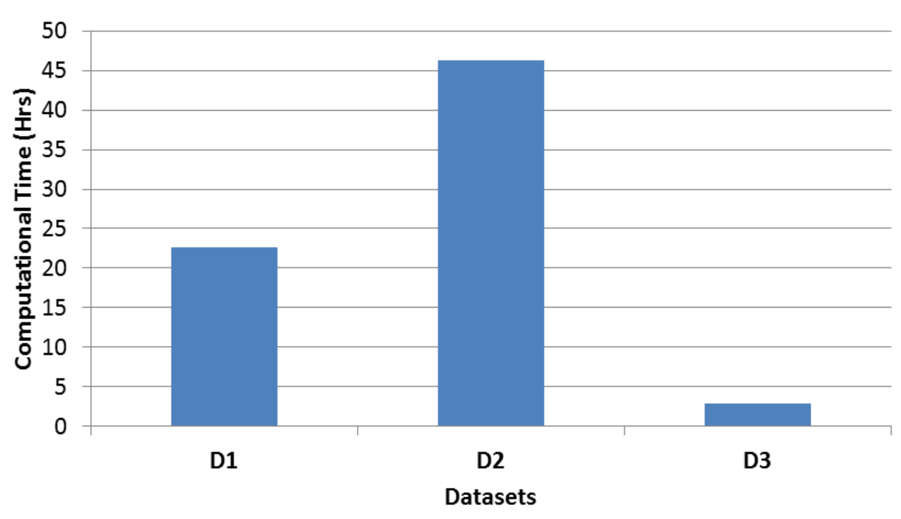
Table 9 gives the computational time complexity for the methods based on dtw. The main computation involved in the use of QS DTW is that of computing the cut specific principal alignments for the frequent classes. Figure 5 shows the time for computing the cut specific principal alignments for the three datasets. The computation of these cut specific principal alignments can be carried out independently for all the classes. Since we can compute these principal alignments in parallel with each other, the proposed QS DTW scales well with the number of samples compared to Fast Apprx dtw [20].
Unlike the case of QS DTW, where the principal alignments are computed for the small cut portions, in Fast Apprx DTW, the principal alignments are computed for the full word image representation. Further, in Fast Apprx DTW, the principal alignments are computed from the entire dataset, unlike the case of QS DTW in which the principal alignments are computed for the individual classes. For these reasons, Fast Apprx DTW is computationally slower compared to the QS DTW.
For a given dataset, computing the cut specific principal alignments for the frequent classes is an offline process. When performing retrieval for a given query, DQC involves computing the query mean by composing together the nearest cut portions from the mean vectors of frequent classes. Further, the query specific principal alignments are not explicitly computed but rather constructed using the cut-specific principal alignments corresponding to the nearest cut portions. Once the query specific principal alignments are obtained, computation of QS DTW involves computing the Euclidean distance (using the query specific principal alignments) with the database images.
For the given two samples x and y of length N, FastDTW [30] is computed in the following way. First, these two samples are reduced to smaller length (1/8 times) and the naive DTW distance is applied over the reduced length samples to find the optimal warp path. Next, both the optimal path and the reduced length samples from the previous step are projected to higher (two times) resolution. Instead of filling all the entries in the cost matrix in the higher resolution, only the entries around a neighborhood of the projected warp path, governed by a parameter called radius r, are filled up. This projection step is continued until the original resolution was obtained. The time complexity of FastDTW is , where r is the radius. The performance of FastDTW depends on the radius r. The higher the value of r, the better the performance is. The time complexity of QSDTW/Fast Apprx DTW is , where p is the number of principal alignments. In general, , for getting the similar performance in both the methods.
6. Conclusions
We have proposed query specific dtw distance for faster indexing in the direct query classifier DQC [18]. The benefit of deploying QS DTW with DQC is that it results in linear time complexity. Therefore, we are able to index all the frequent mean vectors of the database for constructing the mean vector for the query class in the DQC classifier. Since QS DTW distance performs equally well as dtw distance and because we consider all the frequent mean vectors for indexing, the proposed method enhances the performance of the DQC. Unlike previous approaches, the proposed QS DTW distance uses both the class mean vectors and the query information for computing the global principal alignments for the query. The use of ngrams for computing the global principal alignments makes the method perform well for rare queries, which are query word images that belong to non-frequent word classes for which mean vectors are not computed for the database. The query expansion (QE) further improves the performance of QS DTW. We have demonstrated the utility of the proposed technique over three different datasets. The proposed query specific dtw performs well compared to the previous dtw approximations.
Acknowledgments
This work was supported from the grant received for the IMPRINT project titled "Information access from document images of Indian languages," from MHRD, Government of India.
Author Contributions
Gattigorla Nagendar and Viresh Ranjan performed the experiments. Gaurav Harit and C.V Jawahar wrote the paper.
Conflicts of Interest
The authors declare no conflict of interest.
References
- Nagy, G. Twenty Years of Document Image Analysis in PAMI. PAMI 2008, 22, 38–62. [Google Scholar] [CrossRef]
- Sivic, J.; Zisserman, A. Video Google: A Text Retrieval Approach to Object Matching in Videos. In Proceedings of the Ninth IEEE International Conference on Computer Vision, Nice, France, 13–16 October 2003; pp. 1470–1477. [Google Scholar]
- Rath, T.M.; Manmatha, R. Word spotting for historical documents. IJDAR 2007, 9, 139–152. [Google Scholar] [CrossRef]
- Zeki, Y.I.; Manmatha, R. An Efficient Framework for Searching Text in Noisy Document Images. In Proceedings of the 2012 10th IAPR International Workshop on Document Analysis Systems (DAS), Gold Cost, QLD, Australia, 27–29 March 2012; pp. 48–52. [Google Scholar]
- Konidaris, T.; Gatos, B.; Ntzios, K.; Pratikakis, I.; Theodoridis, S.; Perantonis, S.J. Keyword-guided word spotting in historical printed documents using synthetic data and user feedback. IJDAR 2007, 9, 167–177. [Google Scholar] [CrossRef]
- Basilios, G.; Nikolaos, S.; Georgios, L. ICDAR 2009 Handwriting Segmentation Contest. In Proceedings of the 10th International Conference on Document Analysis and Recognition, Barcelona, Spain, 26–29 July 2009; pp. 1393–1397. [Google Scholar]
- Sankar, K.P.; Jawahar, C.V. Probabilistic Reverse Annotation for Large Scale Image Retrieval. In Proceedings of the IEEE Conference on Computer Vision and Pattern Recognition, Minneapolis, MN, USA, 17–22 June 2007. [Google Scholar]
- Almazán, J.; Fernández, D.; Fornés, A.; Lladós, J.; Valveny, E. A Coarse-to-Fine Approach for Handwritten Word Spotting in Large Scale Historical Documents Collection. In Proceedings of the 2012 International Conference on Frontiers in Handwriting Recognition (ICFHR), Bari, Italy, 18–20 September 2012; pp. 455–460. [Google Scholar]
- Yossi, R.; Carlo, T.; Guibas, J.L. The Earth Mover’s Distance As a Metric for Image Retrieval. IJCV 2000, 40, 99–121. [Google Scholar] [CrossRef]
- David, S.; Kruskal, J.B. Time Warps, String Edits, and Macromolecules: The Theory and Practice of Sequence Comparison; Addison-Wesley: Reading, MA, USA, 1983; pp. 1–44. ISBN 0-201-07809-0. [Google Scholar]
- Rath, T.M.; Manmatha, R. Word Image Matching Using Dynamic Time Warping. In Proceedings of the 2003 IEEE Computer Society Conference on Computer Vision and Pattern Recognition, Madison, WI, USA, 18–20 June 2003; pp. 521–527. [Google Scholar]
- Tomasz, M.; Abhinav, G.; Efros, A.A. Ensemble of exemplar-SVMs for Object Detection and Beyond. In Proceedings of the 2011 International Conference on Computer Vision, Barcelona, Spain, 6–13 November 2011; pp. 89–96. [Google Scholar]
- Cao, H.; Govindaraju, V. Vector Model Based Indexing and Retrieval of Handwritten Medical Forms. In Proceedings of the Ninth International Conference on Document Analysis and Recognition, Parana, Brazil, 23–26 September 2007; pp. 88–92. [Google Scholar]
- Rath, T.M.; Manmatha, R. Features for Word Spotting in Historical Manuscripts. In Proceedings of the Seventh International Conference on Document Analysis and Recognition, Edinburgh, UK, 6 August 2003. [Google Scholar]
- Balasubramanian, A.; Million, M.; Jawahar, C.V. Retrieval from Document Image Collections. In Proceedings of the 7th International Workshop, DAS 2006, Nelson, New Zealand, 13–15 February 2006; pp. 1–12. [Google Scholar]
- Kovalchuk, A.; Wolf, L.; Dershowitz, N. A Simple and Fast Word Spotting Method. In Proceedings of the 2014 14th International Conference on Frontiers in Handwriting Recognition (ICFHR), Heraklion, Greece, 1–4 September 2014; pp. 3–8. [Google Scholar]
- Shai, S.; Yoram, S.; Nathan, S. Pegasos: Primal Estimated sub-GrAdient Solver for SVM. In Proceedings of the 24th International Conference on Machine Learning, Corvalis, OR, USA, 20–24 June 2007; pp. 807–814. [Google Scholar]
- Ranjan, V.; Harit, G.; Jawahar, C.V. Document Retrieval with Unlimited Vocabulary. In Proceedings of the 2015 IEEE Winter Conference on Applications of Computer Vision (WACV), Waikoloa, HI, USA, 5–9 January 2015; pp. 741–748. [Google Scholar]
- Nagendar, G.; Jawahar, C.V. Fast Approximate Dynamic Warping Kernels. In Proceedings of the Second ACM IKDD Conference on Data Sciences, Bangalore, India, 18–21 March 2015; pp. 30–38. [Google Scholar]
- Nagendar, G.; Jawahar, C.V. Efficient word image retrieval using fast DTW distance. In Proceedings of the 2015 13th International Conference on Document Analysis and Recognition (ICDAR), Tunis, Tunisia, 23–26 August 2015; pp. 876–880. [Google Scholar]
- Sudholt, S.; Fink, G.A. PHOCNet: A Deep Convolutional Neural Network for Word Spotting in Handwritten Documents. In Proceedings of the 2016 15th International Conference on Frontiers in Handwriting Recognition (ICFHR), Shenzhen, China, 23–26 October 2016; pp. 686–690. [Google Scholar]
- Krishnan, P.; Dutta, K.; Jawahar, C.V. Deep Feature Embedding for Accurate Recognition and Retrieval of Handwritten Text. In Proceedings of the 2016 15th International Conference on Frontiers in Handwriting Recognition (ICFHR), Shenzhen, China, 23–26 October 2016; pp. 686–690. [Google Scholar]
- Jon, A.; Albert, G.; Alicia, F.; Ernest, V. Word Spotting and Recognition with Embedded Attributes. IEEE Trans. Pattern Anal. Mach. Intell. 2014, 36, 2552–2566. [Google Scholar]
- Sfikas, G.; Giotis, A.P.; Louloudis, G.; Gatos, B. Using attributes for word spotting and recognition in polytonic greek documents. In Proceedings of the 2015 13th International Conference on Document Analysis and Recognition (ICDAR), Tunis, Tunisia, 23–26 August 2015; pp. 686–690. [Google Scholar]
- Almazán, J.; Gordo, A.; Fornés, A.; Valveny, E. Segmentation-free Word Spotting with Exemplar SVMs. Pattern Recognit. 2014, 47, 3967–3978. [Google Scholar] [CrossRef]
- Takami, M.; Bell, P.; Ommer, P. Offline learning of prototypical negatives for efficient online Exemplar SVM. In Proceedings of the 2014 IEEE Winter Conference on Applications of Computer Vision (WACV), Steamboat Springs, CO, USA, 24–26 March 2014; pp. 377–384. [Google Scholar]
- Gharbi, M.; Malisiewicz, T.; Paris, S.; Durand, F. A Gaussian Approximation of Feature Space for Fast Image Similarity; MIT CSAIL Technical Report; CSAIL Publications: Cambridge, MA, USA, 2012. [Google Scholar]
- Meinard, M. Information Retrieval for Music and Motion; Springer: Secaucus, NJ, USA, 2007; pp. 32–58. ISBN 3540740473. [Google Scholar]
- Muja, M.; Lowe, D.G. Fast approximate nearest neighbours with automatic algorithm configuration. In Proceedings of the 4th International Conference on Computer Vision Theory and Applications, Lisboa, Portugal, 5–8 February 2009; pp. 331–340. [Google Scholar]
- Stan, S.; Philip, C. Fastdtw: Toward accurate dynamic time warping in linear time and space. In Proceedings of the KDD Workshop on Mining Temporal and Sequential Data, Seattle, WA, USA, 22 August 2004. [Google Scholar]
- Fischer, A.; Keller, A.; Frinken, V.; Bunke, H. Lexicon-free handwritten word spotting using character HMMs. Pattern Recognit. Lett. 2012, 33, 934–942. [Google Scholar] [CrossRef]
Figure 1.
Figure shows few query words and their corresponding retrieval results. The first column shows the query image and the corresponding images in each row are its retrieval results. First two rows show frequent query results. The first row shows the results for NN DQC and second row show the results for DP DQC. Row 3 to Row 5 show the retrieval results for a rare query. Row 3 shows the results for NN DQC and Row 4 show the results for DP DQC and Row 5 show the results for query expansion.

Figure 2.
The top alignments between few samples from 2 different classes. Here, X-axis is the length of the samples from class 1 and Y-axis is the length of the samples from class 2.
Figure 2.
The top alignments between few samples from 2 different classes. Here, X-axis is the length of the samples from class 1 and Y-axis is the length of the samples from class 2.
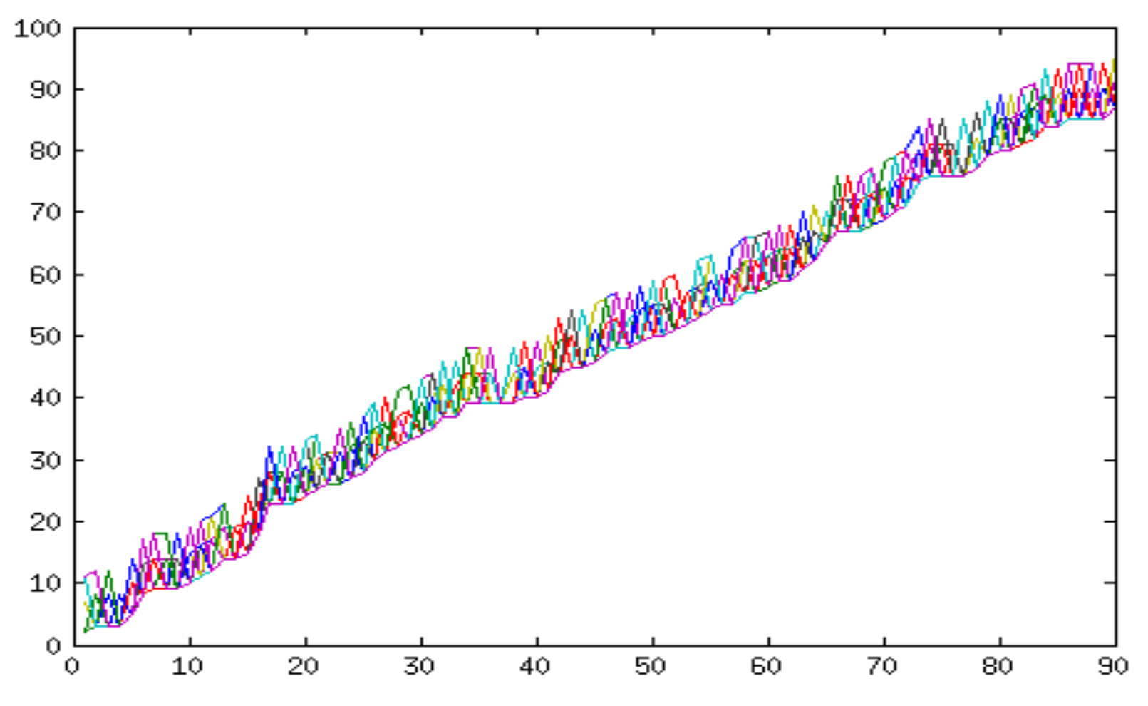
Figure 3.
Overall Scheme for NN DQC. In an offline phase, the mean vectors for the frequent word classes are computed and their cut-specific principal alignments are computed. To process a query word image, it is divided into cut portions and Fastdtw matching is used to get the best matching cut-portions from the frequent class mean vectors with the cut-portions of the query image. These best matching cut-portions are used to construct the mean vector for the query class and the query specific principal alignments. Fastdtw [20] matching between the query image and the database images is done using the query specific principal alignments.
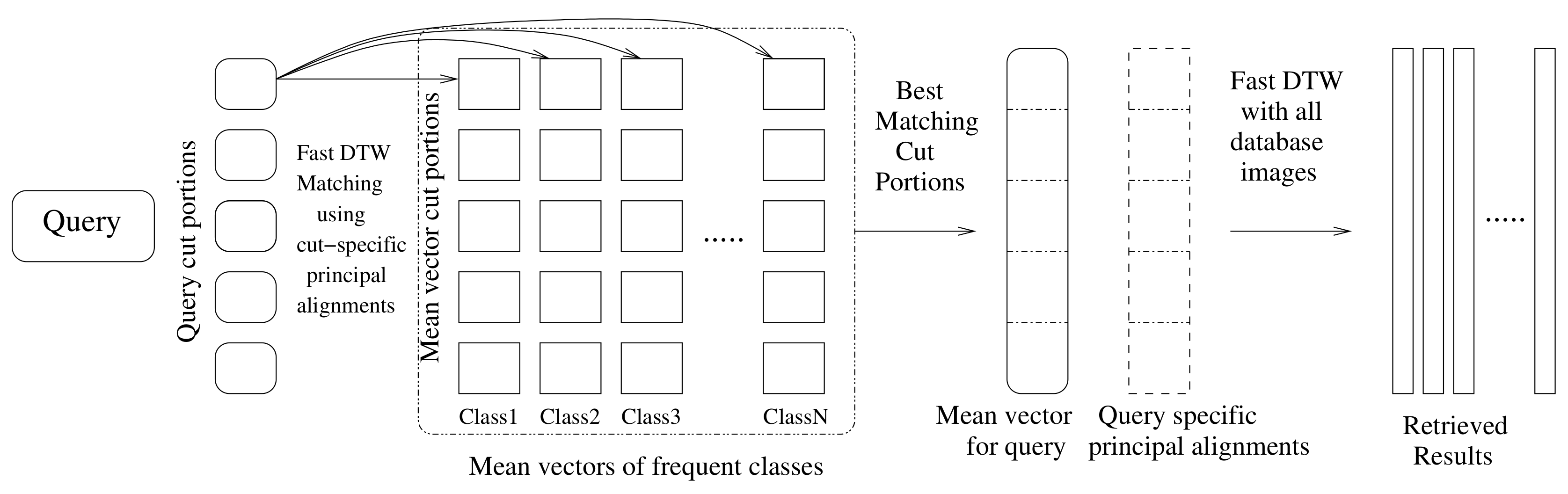
Figure 4.
Synthesis of query specific principal alignments. (a) Cut specific principal alignments corresponding to “ground” and “leather” are joined to form the principal alignments for “great”. Note that the appropriate cut portions are automatically found. (b) In a general setting, query specific principal alignments gets formed from multiple constituent cut specific principal alignments computed for frequent classes.
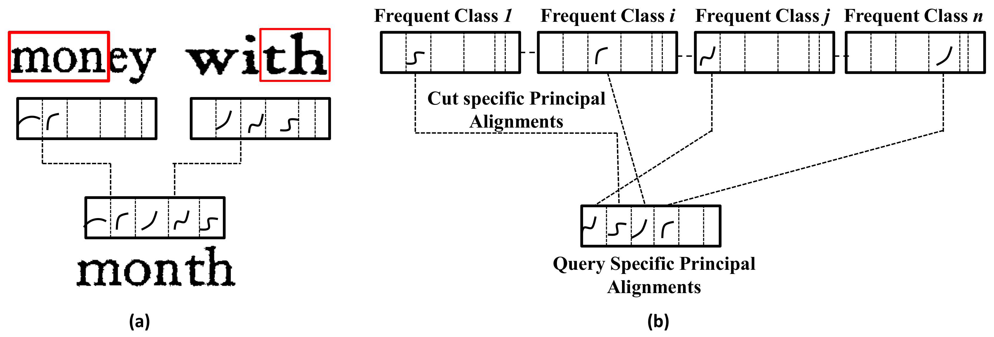
Figure 5.
Computation time for computing the cut specific principal alignments for all the datasets. It includes the computation of cut specific principal alignments for all the frequent classes over all the cut portions.
Figure 5.
Computation time for computing the cut specific principal alignments for all the datasets. It includes the computation of cut specific principal alignments for all the frequent classes over all the cut portions.

Table 1.
The comparison of the performance of DTW distance, Fast Apprx DTW and Euclidean distance as a similarity measure for a word retrieval problem.
Table 1.
The comparison of the performance of DTW distance, Fast Apprx DTW and Euclidean distance as a similarity measure for a word retrieval problem.
| dtw Distance | Fast Apprx dtw | Euclidean | |
|---|---|---|---|
| mAP score | 0.96 | 0.94 | 0.82 |
Table 2.
Details of the datasets considered in the experiments. The first collection (D1) of words is from a book which is reasonably clean. The second dataset (D2) is obtained from 2 books and is used to demonstrate the performance in case of heterogeneous print styles. The third dataset (D3) is a noisy book.
| Dataset | Source | Type | # Images | # Queries |
|---|---|---|---|---|
| D1 | 1 Book | Clean | 14,510 | 100 |
| D2 | 2 Books | Clean | 32,180 | 100 |
| D3 | 1 Book | Noisy | 4100 | 100 |
Table 3.
Retrieval performance of various methods for frequent queries.
| Dataset | Retrieval Results (mAP) for Frequent Queries | ||||||||
|---|---|---|---|---|---|---|---|---|---|
| Using Nearest Neighbour Classifier | Using dqc (Exemplar SVM) | ||||||||
| dtw | Fast Apprx dtw [20] | qs dtw | Euclidean | Fastdtw [30] | sdtw | ann | Fastdtw | qs dtw | |
| D1 | 0.94 | 0.92 | 0.92 | 0.81 | 0.91 | 0.98 | 0.98 | 1 | 1 |
| D2 | 0.91 | 0.89 | 0.9 | 0.75 | 0.87 | 0.96 | 0.95 | 0.97 | 0.99 |
| D3 | 0.83 | 0.79 | 0.81 | 0.67 | 0.76 | 0.91 | 0.92 | 0.93 | 0.96 |
Table 4.
Retrieval performance of various methods for rare queries.
| Dataset | Retrieval Results (mAP) for Rare Queries | |||||||||
|---|---|---|---|---|---|---|---|---|---|---|
| Using Nearest Neighbour Classifier | Using dqc (Exemplar SVM) | |||||||||
| dtw | Fast Apprx dtw [20] | qs dtw | Euclidean | Fastdtw [30] | sdtw | ann | Fastdtw | qs dtw | QE | |
| D1 | 0.82 | 0.77 | 0.83 | 0.69 | 0.75 | 0.91 | 0.90 | 0.91 | 0.95 | 0.98 |
| D2 | 0.81 | 0.74 | 0.80 | 0.65 | 0.74 | 0.89 | 0.90 | 0.90 | 0.94 | 0.95 |
| D3 | 0.73 | 0.66 | 0.71 | 0.59 | 0.62 | 0.80 | 0.78 | 0.80 | 0.91 | 0.96 |
Table 5.
The table gives the average sum of dtw distance for the given query and the reformulated query with varying number of samples n from the query class.
Table 5.
The table gives the average sum of dtw distance for the given query and the reformulated query with varying number of samples n from the query class.
| Average of dtw Distance | ||||
|---|---|---|---|---|
| For given query | For Reformulated Query | |||
| n = 2 | n = 5 | n = 7 | n = 10 | |
| 2.67 ± 0.19 | 2.69 ± 0.23 | 2.52 ± 0.13 | 2.58 ± 0.21 | 2.94 ± 0.29 |
Table 6.
Retrieval performance on the George Washington (GW) dataset. The dqc makes use of top 800 frequent classes for indexing the cut-portions.
Table 6.
Retrieval performance on the George Washington (GW) dataset. The dqc makes use of top 800 frequent classes for indexing the cut-portions.
| Dataset | mAP Using Nearest Neighbour | mAP Using dqc | |||||
|---|---|---|---|---|---|---|---|
| dtw | Fast Apprx dtw [20] | qs dtw | Euclidean | sdtw | Fastdtw [30] | qs dtw | |
| gw | 0.51 | 0.50 | 0.52 | 0.32 | 0.62 | 0.63 | 0.70 |
Table 7.
The table shows the change in retrieval performance with the change in the length of cut portion over all the datasets (D1, D2, D3). Here l is the length of the cut portion.
Table 7.
The table shows the change in retrieval performance with the change in the length of cut portion over all the datasets (D1, D2, D3). Here l is the length of the cut portion.
| l | D1 | D2 | D3 |
|---|---|---|---|
| 1 | 0.81 | 0.78 | 0.7 |
| 10 | 0.86 | 0.83 | 0.74 |
| 20 | 0.86 | 0.82 | 0.75 |
| 30 | 0.82 | 0.77 | 0.72 |
Table 8.
Retrieval performance on the 3 datasets D1, D2 and D3 for varying number of cut specific principal alignments.
Table 8.
Retrieval performance on the 3 datasets D1, D2 and D3 for varying number of cut specific principal alignments.
| Number of Cut Specific Principal Alignments | mAP for Different Datasets | ||
|---|---|---|---|
| D1 | D2 | D3 | |
| 10 | 0.92 | 0.89 | 0.81 |
| 20 | 0.93 | 0.89 | 0.81 |
| 30 | 0.91 | 0.88 | 0.78 |
Table 9.
Computational complexities of dtw-based methods for distance computation. Here n is the length of the cut-portion of the feature vector.
© 2018 by the authors. Licensee MDPI, Basel, Switzerland. This article is an open access article distributed under the terms and conditions of the Creative Commons Attribution (CC BY) license (http://creativecommons.org/licenses/by/4.0/).
Share and Cite
MDPI and ACS Style
Nagendar, G.; Ranjan, V.; Harit, G.; Jawahar, C.V. Efficient Query Specific DTW Distance for Document Retrieval with Unlimited Vocabulary. J. Imaging 2018, 4, 37. https://0-doi-org.brum.beds.ac.uk/10.3390/jimaging4020037
AMA Style
Nagendar G, Ranjan V, Harit G, Jawahar CV. Efficient Query Specific DTW Distance for Document Retrieval with Unlimited Vocabulary. Journal of Imaging. 2018; 4(2):37. https://0-doi-org.brum.beds.ac.uk/10.3390/jimaging4020037
Chicago/Turabian StyleNagendar, Gattigorla, Viresh Ranjan, Gaurav Harit, and C. V. Jawahar. 2018. "Efficient Query Specific DTW Distance for Document Retrieval with Unlimited Vocabulary" Journal of Imaging 4, no. 2: 37. https://0-doi-org.brum.beds.ac.uk/10.3390/jimaging4020037
Note that from the first issue of 2016, this journal uses article numbers instead of page numbers. See further details here.