Article

Faster R-CNN-Based Glomerular Detection in Multistained Human Whole Slide Images

1
Department of Healthcare Information Management, The University of Tokyo Hospital, Tokyo 113-8655, Japan
2
Department of Biomedical Informatics, Graduate School of Medicine, The University of Tokyo, Tokyo 113-8655, Japan
3
Department of Pathology, Graduate School of Medicine, The University of Tokyo, Tokyo 113-8655, Japan
4
Department of Pathology, Teikyo University School of Medicine, Tokyo 173-8605, Japan
*
Author to whom correspondence should be addressed.
Submission received: 16 May 2018 / Revised: 13 June 2018 / Accepted: 2 July 2018 / Published: 4 July 2018
(This article belongs to the Special Issue Medical Image Analysis)

Abstract

:
The detection of objects of interest in high-resolution digital pathological images is a key part of diagnosis and is a labor-intensive task for pathologists. In this paper, we describe a Faster R-CNN-based approach for the detection of glomeruli in multistained whole slide images (WSIs) of human renal tissue sections. Faster R-CNN is a state-of-the-art general object detection method based on a convolutional neural network, which simultaneously proposes object bounds and objectness scores at each point in an image. The method takes an image obtained from a WSI with a sliding window and classifies and localizes every glomerulus in the image by drawing the bounding boxes. We configured Faster R-CNN with a pretrained Inception-ResNet model and retrained it to be adapted to our task, then evaluated it based on a large dataset consisting of more than 33,000 annotated glomeruli obtained from 800 WSIs. The results showed the approach produces comparable or higher than average F-measures with different stains compared to other recently published approaches. This approach could have practical application in hospitals and laboratories for the quantitative analysis of glomeruli in WSIs and, potentially, lead to a better understanding of chronic glomerulonephritis.

Graphical Abstract

1. Introduction

1.1. Detection of Glomeruli in Whole Slide Images

Chronic glomerulonephritis (CGN) refers to several kidney diseases in which the glomerulus is damaged by continuous inflammation and its ability to filter the blood decreases. The progression of CGN may lead to kidney failure, requiring dialysis or transplantation to maintain life. Detecting CGN at an early stage in order to make an appropriate intervention is important for improving the quality of life of patients and reducing social costs. Pathological examination is often required for precise diagnosis of CGN. A pathological sample (microscope slide), containing a few sections of human kidney tissue obtained by puncture biopsy, is prepared. The pathologist observes the sample with a microscope and finds morphological features of glomeruli over the whole area of the sample. Finally, a clinical diagnosis is carried out together with the features of the glomeruli and clinical findings, such as the course of the disease and the results of blood and urine tests. In recent years, digital pathology has become widespread in the field of renal pathology. A histopathological whole slide image (WSI) is obtained by scanning the microscope slide to produce digital slides to be viewed by humans or to be subjected to computerized image analysis. The WSI has been useful for telepathology, educational applications, research purposes, and computer-supported pathological diagnosis systems [1,2,3].
The detection of glomeruli is an important step in developing rapid and robust diagnostic tools that detect multiple glomeruli contained in the WSI and in proposing a classification of morphological features of the glomeruli. The present study addresses the task of detecting glomeruli from the WSI. Compared with general object detection tasks, glomerular detection from the WSI has three major difficulties. First, the size of the WSI is relatively large, and it is necessary to find an efficient method to detect minute glomeruli in this image. Our WSI is a 40-times magnified image that has a long side exceeding 220,000 pixels, and the direct use of an image of this size is not efficient, even with a modern computer. Therefore, down-sampling of the WSI to an appropriate resolution and use of the sliding window method should be applied to the WSI. Second, although the glomerulus is a spherical tissue, the two-dimensional image of the glomerulus varies in size and shape. This is due to variations in the slicing angle and pressure when obtaining thin samples. In addition, because WSIs obtained from clinical practice contain not only normal glomeruli but also many abnormal glomeruli, the texture and the internal structure of the glomeruli are more variable, and these characteristics make it difficult to detect glomeruli. Finally, because the diagnosis of renal pathology requires multiple stained images, the method of glomerular detection should be robust against variations caused by differences in staining.

1.2. Digital Pathology Analysis with Deeply Multilayered Neural Network (DNN)

Deep learning is a technique to efficiently train a DNN model that imitates the signal transduction of nerve cells. The use of DNNs has been spreading rapidly in recent years because it has shown better performance than conventional machine learning methods in tasks for recognition of images [4,5] and speech [6,7] and for machine translation [8,9]. Because the output of the neural network (NN) depends on the connection weights between the artificial neurons, optimizing the weights to obtain the desired output corresponds to training the NN. In typical use of an NN, supervised learning is employed. During training of the NN under supervised learning, the input vector is presented to the network, which will produce an output vector. This output vector is compared with the desired output vector, and an error signal between the actual output and the desired output is evaluated. Based on this error signal, the connection weights are updated by a back-propagation method until the actual output is matched with the desired output. Among DNNs, the convolutional neural network (CNN) is specially designed for the recognition of images that have strong correlations with neighboring data. A typical CNN architecture consists of convolutional layers, pooling layers, and a fully connected layer. Convolutional layers extract features of the input image by scanning the filters over the entire image and passing the results (called feature maps) to the next layer. Pooling layers are placed after convolutional layers mainly to reduce the dimensionality of the feature map, which can in turn improve robustness to spatial variations such as shifting or scaling of the features in the image. The convolutional and pooling layers are often repeated several times, and the results are passed to the fully connected layers which is the same as the traditional multilayer NN to output vector. In recent years, CNNs have contributed to various generic tasks in the field of digital medical image analysis [10,11,12], image classification, object detection, and object segmentation. Image classification is a popular task performed by CNN that classifies an input image into multiple classes. For example, classification of leukemia cells [13] and classification of cell nuclei in colon tissue [14] are performed by CNN. Although the classification is useful when an image contains one object of interest, object detection or object segmentation plays a more important role when an image contains multiple objects. In particular, detection of objects of interest or lesions in high-resolution digital pathological images is a key part of diagnosis and is one of the most labor-intensive tasks for pathologists. Object detection involves not only recognizing and classifying every object in an image, but also localizing each one by drawing a bounding box around it. On the other hand, although its purpose is somewhat like that of object detection, object segmentation draws the boundary of an object or background by classifying each pixel of the image into multiple classes. These make object detection or object segmentation significantly more difficult than image classification. Object detection of mitotic cells in breast cancer tissue [15,16,17] and semantic segmentation to identify the site of cancer in colon tissue [18] were performed in the field of digital pathological image analysis.

1.3. Previous Work

We describe below previous studies focused on the tasks of glomerular detection in the WSIs of renal biopsies. A few studies have directly addressed the problem of simultaneous detection and classification of glomeruli. Our study was conducted on human kidney tissue, but the following studies include those performed on the kidneys of mice and rats.

1.3.1. Hand-Crafted Feature-Based Methods

The histogram of oriented gradients (HOG) [19] is a hand-crafted feature that is widely used in object detection tasks. First, the HOG divides an image into rectangular regions of an appropriate size called cells and calculates the gradient of intensity within each cell by a histogram. Next, a block is composed of a neighboring cell, and the value of the histogram is normalized within the block, thereby obtaining the HOG feature for one cell. The standard HOG is called the rectangle-HOG (R-HOG), because the cells are arranged in a lattice pattern to form a block. In [20], the authors proposed a method of detecting glomeruli by R-HOG with a SVM (support vector machine) for the WSIs of renal biopsy specimens obtained from rats. This study pointed out the problem that because the extracted features differ greatly between blocks on the inside and the outside of the glomerulus, robustness against deformity of the glomerulus is decreased. To address this problem, the authors proposed a method using segmental-HOG (S-HOG) that arranges blocks in a more flexible manner radially rather than in a lattice [21]. In this method, the image is scanned by the sliding window, the window containing the glomerulus is screened by R-HOG with SVM, and then the glomeruli or the background are classified further by S-HOG with SVM to reduce the number of false positive (FP) cases. Although the S-HOG does not simply replace the R-HOG, the F-measures of glomerular detection from the WSIs of rat kidney by R-HOG with SVM and S-HOG with SVM were 0.838 and 0.866, respectively, and S-HOG was reported to be effective.
Another study [22] proposed a method of glomerular detection using the local binary patterns (LBP) image feature vector to train an SVM. The multi-radial color LBP (mrcLBP) calculates LBP descriptors for four different radii per center pixel, as well as for each RGB color channel, then, concatenates the resulting 12 descriptors to create a 120-dimensional feature vector. In the training of the SVM classifier, mrcLBP features are extracted from glomerular images and background images cropped by the WSI at a fixed-sized window (576 × 576 pixels, 144 × 144 µm). At the time of evaluation, the sliding window approach was employed with the same-sized window, the score of the likelihood of a glomerulus was calculated by the trained SVM, and the glomerulus was detected through multiple threshold processing of the score. The experiments were conducted using the WSIs obtained from multiple species (human, rat, and mouse) and with multiple stains (hematoxylin and eosin (HE), periodic acid-Schiff (PAS), Jones silver (JS), Gömöri’s trichrome (TRI) and Congo red (CR)). The F-measure of mrcLBP with SVM was reported as 0.850 in mouse HE stain, 0.680–0.801 in rat HE, PAS, JS, TRI and CR stains, and 0.832 in human PAS stain, respectively.

1.3.2. Convolutional Neural Network (CNN) Based Methods

Some recent studies employed mainly CNN for glomerular detection. In [23], the authors evaluated the difference in performance between the HOG with the SVM classifier and the three-layered CNN classifier for glomerular detection in WSIs with multiple stains. They employed the sliding window approach to scan the WSIs. The window size was fixed at 128 × 128 pixels. The results showed the F-measures of the HOG with the SVM were 0.405 to 0.551, and the F-measures of CNN were 0.522 to 0.716, indicating CNN had an advantage of approximately 10% to 20% compared to the HOG with the SVM classifier. They proposed also a method of combining consecutive sections stained with different histochemical stains to reduce FP cases by leaving only detection results supported by images with different stains. Although this method requires complicated processing to acquire combined consecutive sections, the results showed some stains were effective. More recently, the authors proposed a straightforward method of glomerular detection using a CNN classifier by scanning the WSI with a fixed-sized sliding window and classifying the images contained in the window as glomeruli or background [24]. After training a CNN classifier, the authors applied a sliding window approach of 227 × 227 pixels with 80% overlapping in both the row and column directions. A maximum of 25 (5 × 5) classifications were performed on a small square region, and whether the region contained a glomerulus was determined by the ensemble of classifications. Although the results obtained by this method seem to provide coarse object segmentation rather than object detection, the F-measure with PAS staining was reported as 0.937. Table 1 shows a summary of the previous studies mentioned above.

1.4. Objective

This study addresses the detection of glomeruli from the WSIs by applying Faster R-CNN [25], which is designed for general object detection. In our approach, Faster R-CNN takes a fixed-sized image obtained from a WSI with sliding window, and classifies and localizes every glomerulus in the image by drawing bounding boxes. After the detection of the glomeruli for all images in a WSI, overlapping bounding boxes located at the boundaries of the windows are merged to avoid duplicate detection. Performance is measured by evaluating whether the proposed bounding boxes overlap sufficiently with bounding boxes that are given as ground truth. We evaluated the detection accuracy of Faster R-CNN for the WSIs with four kinds of stains and examined how many WSIs were required to obtain sufficient accuracy. Below, we briefly indicate contributions of previous and present works.
What was already known on the topic:
  • In glomerular detection from human WSIs, recent publications have reported that a CNN-based approach showed the F-measures 0.937 and a handcraft feature-based approaches (mrcLBP with SVM) showed 0.832 in PAS stain.
What this study added to our knowledge:
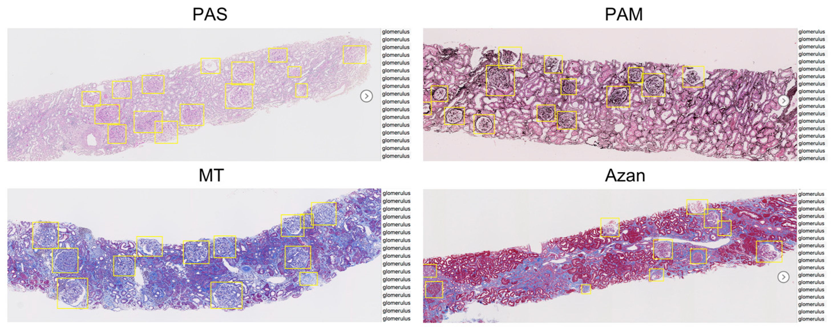
  • Our approach based on a Faster-RCNN showed the F-measures 0.925 in PAS stain. It also showed equally high performance can be obtained not only for PAS stain but also for PAM (0.928), MT (0.898), and Azan (0.877) stains.
  • As for the required number of WSIs used for the network training, the F-measures were saturated with 60 WSIs in PAM, MT, and Azan stains. However, it was not saturated with 120 WSIs in the PAS stain.

2. Materials and Methods

2.1. Datasets

A total of 800 renal biopsy microscope slides collected at the University of Tokyo hospital during the period from 2010 to 2017 were used. Because these slides were obtained in a clinical setting, the patients suffered from various diseases. We used multiple stained microscope slides to evaluate the robustness of the accuracy of glomerular detection to diverse slide-staining methods. The slides included four kinds of stain: PAS (periodic acid-Schiff), PAM (periodic acid-methenamine silver), MT (Masson trichrome), and Azan. The pictorial features of each stain are as follows. PAS is widely used for glomerular observation and is mainly used for evaluating the mesangial region by highlighting the glycoprotein in red. PAM stains collagen darkly and is used mainly for evaluating the basement membrane of the glomerulus. MT and Azan are used mainly to evaluate sclerosis or fibrosis of the glomerulus by making these regions blue and red, respectively. Pathological sample collection followed a protocol approved by the Institutional Review Board at the University of Tokyo Hospital (Approval Number: 11455). All methods described below were carried out in accordance with the relevant ethical guidelines and regulations.
To produce WSIs by scanning microscope slides, a Hamamatsu NanoZoomer 2.0 HT (Hamamatsu Photonics KK) was used. The WSIs were provided by a file with NDPI file extension, which includes an image taken by a 40× objective lens magnification, with a resolution 0.23 µm/pixel. With this resolution, the maximum image size is 225,000 × 109,000 pixels (51,750 × 25,070 µm), too large to be directly handled efficiently. Therefore, we down-sampled the WSIs to the equivalent of 5× magnification, large enough to allow the detection of glomeruli by humans, and converted them to PNG file format with OpenSlide [26]. Consequently, the scale of the WSIs became 1.82 µm/pixel, that is, the average, maximum, and minimum sizes were 16,733 × 4005, 28,160 × 13,728, and 1536 × 1248 pixels, respectively. The annotation for object detection by bounding boxes requires the location of four vertex and class labels as supervised data. Two physicians and an assistant manually annotated glomerular regions by bounding boxes in 800 WSIs under the supervision of a nephrologist (Figure 1). The whole dataset includes approximately 33,000 glomeruli. A summary of the dataset is shown in Table 2.

2.2. Faster R-CNN

Multiple object detection methods based on CNN have been proposed: R-CNN [27], SPPnet [28], Fast R-CNN [29], Faster R-CNN [25], You Only Look Once (YOLO) [30], and Single shot multibox detector (SSD) [31]. Faster R-CNN has state-of the art performance, although its processing speed is lower than that of the more recent methods YOLO and SSD. Because the processing speed is not so important for the purpose of our application, we used Faster R-CNN, which has high performance and does not specify the size of the input image, which is advantageous for handling large images with the sliding window. Here, we introduce the key aspects of Faster R-CNN briefly. Faster R-CNN consists of two modules, the region proposal network (RPN), which identifies the region of the object on the image, and a network that classifies the objects in the proposed region. Faster R-CNN first processes the input image with a feature extractor, which is a CNN consisting of a convolution layer and a pooling layer, to obtain feature maps and pass them to the RPN. Although the original Faster R-CNN used the Simonyan and Zisserman model (VGG-16) [5] as the feature extractor, this CNN can be replaced with a different model. We used Inception-ResNet [32], which has higher performance than the VGG-16. Next, the RPN scans over the feature maps by the sliding window and calculates two scores that indicate whether each window contains an object and whether the object is a background or not. In the sliding window process, it is difficult to detect objects of various shapes by scanning with a fixed-sized window. To deal with various shapes of objects, multiple k windows called anchor boxes, which have different scales and aspect ratios are introduced. Consequently, 4 × k pieces of area information and 2 × k pieces of class information are obtained for each central point of the sliding window. For example, if the size of the feature maps is W × H, approximately 4 k × W × H pieces of area information and 2 k × W × H pieces of class information are output from the RPN. In the original setting, 9 anchor boxes (k = 9) were used, but to detect more forms of glomeruli, we used 12 anchor boxes (k = 12), which consist of 4 kinds of scales and 3 kinds of aspect ratios. Candidate regions obtained by RPN are redundant, because RPN proposes multiple regions for the same object. In order to solve this redundancy, non-maximum suppression based on the class score is employed, which narrows the number of regions of interest (ROIs) down to approximately 300. Because the ROIs are of different sizes, they are converted into fixed-sized vectors through ROI pooling [27] to be input to a fully connected layer. Finally, in the fully connected layer, bounding box regression and n + 1 object classification (adding background to object class n) are conducted in a supervised fashion.

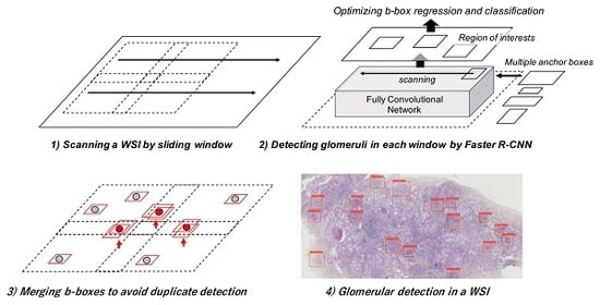
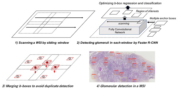
2.3. Glomerular Detection Process from Whole Slide Images (WSIs)

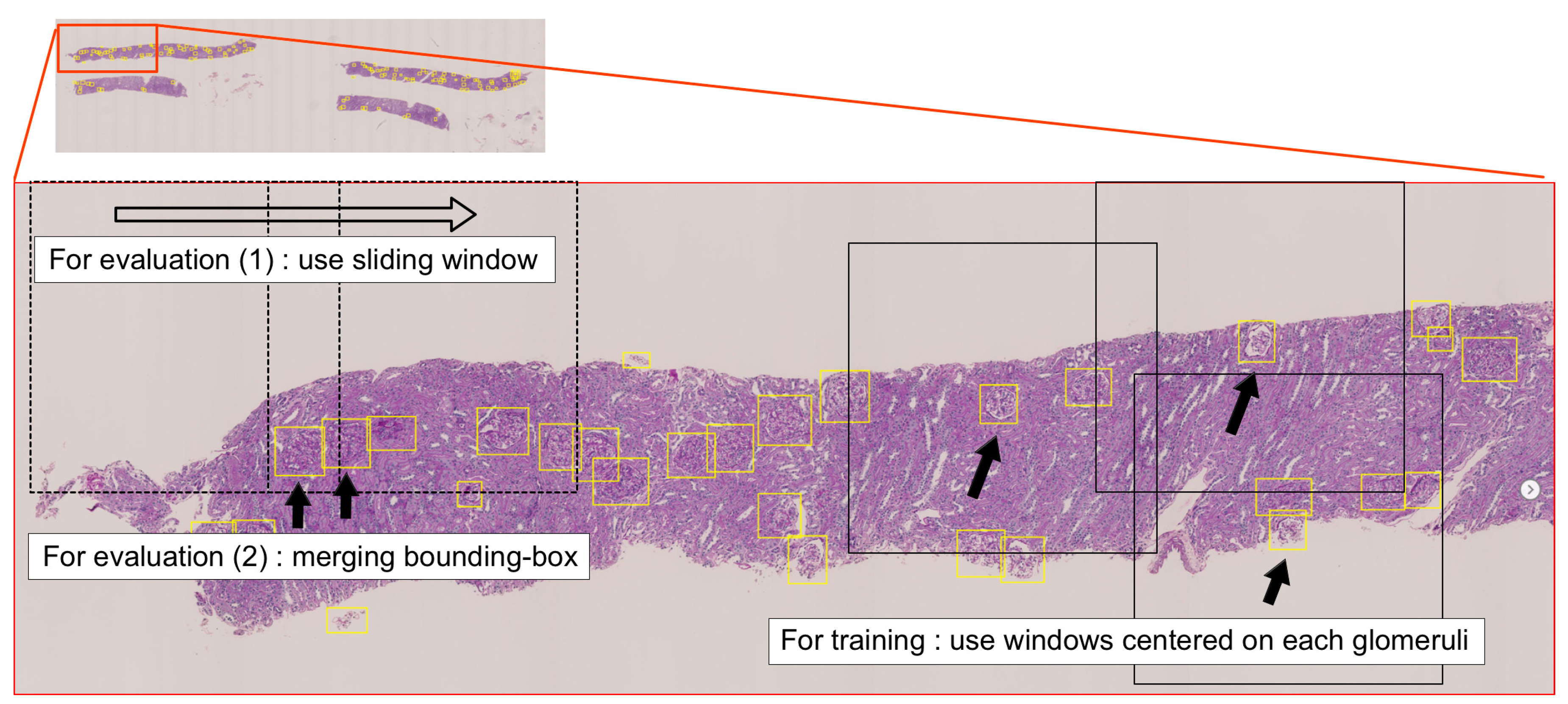
2.3.1. Sliding Window Method for WSIs

We conducted glomerular detection with down-sampled WSIs equivalent to 5× objective lens magnification. If the size of the down-sampled WSI was too large to input the whole image into the NN, we employed a sliding window approach. We estimated the diameter of the glomerulus as approximately 55 pixels (100 µm) to 110 pixels (200 µm) and set the window size to 1099 × 1099 pixels (2000 × 2000 µm) so that multiple glomeruli could be included in a window. For training the Faster R-CNN model, images cropped by the windows centered on each annotated glomerulus were fed to the network. The incomplete glomerular bounding boxes located at the boundaries of the windows were ignored. In evaluating the model, the whole area of the WSI was scanned by the sliding window (row-by-row, left-to-right), and the image contained in the window was taken as input. Neighboring windows were scanned overlapping each other by 10% (200 µm, 110 pixels), so that all of a glomerulus could be included in a window even if it was located at the boundary of the window. Consequently, it was possible to reduce variations in shape of the glomeruli to be detected, while increasing the chance of detecting a glomerulus multiple times at the overlapping regions. Thus, when a detected glomerulus was located in the overlapping region of neighboring windows, bounding boxes overlapping by 35% or more were merged into one. Figure 2 is an overview of the glomerular detection process.

2.3.2. Evaluation Metrics

The glomerular detection that we perform is a binary classification task that evaluates whether Faster R-CNN can correctly detect bounding boxes surrounding the glomeruli given as ground truth. For this reason, micro-averages of recall, precision, and their harmonic mean (F-measure) were used as evaluation metrics. In the micro-average method, the individual true positive (TP), FP, and false negative (FN) cases for all WSIs are summed up and are applied to obtain the statistics. TP is the case in which the proposed bounding box sufficiently overlaps with the ground truth. FP is the case in which the proposed bounding box overlaps with the ground truth insufficiently. FN is the ground truth that could not be detected. To determine whether the proposed bounding box overlaps with the ground truth sufficiently, we used intersection over union (IoU), which is an evaluation metric used to measure the accuracy of detection of an object. This evaluation metric is often used in object detection contests such as the PASCAL Visual Object Classes (PASCAL VOC) challenge [33]. The IoU is obtained by dividing the area of overlap between the bounding boxes by the area of union. We set the threshold of the IoU to 0.5, according to the configuration of the PASCAL VOC challenge. On the other hand, since the likelihood of detecting a glomerulus is given as a probability ranging from 0 to 1, detection performance can be changed by providing a threshold. If the threshold is lowered, objects closer to the background will be detected as glomeruli, which leads to higher recall and lower precision. Conversely, a higher threshold leads to lower recall and higher precision. Thus, we considered this threshold as one of the hyperparameters and set the threshold to maximize F-measure in the experiment described below.

2.3.3. Faster R-CNN Training

We used Faster R-CNN implementation provided by Tensorflow Object Detection API, which is a deep learning framework with Python language. We applied a technique called fine tuning that takes a pretrained model and transfers the connection weights to our own model, retraining the model to be adapted to our task. The pretrained model had been trained on Common Objects in Context (COCO) [34], which is a large image dataset designed for object detection and object segmentation. Fine tuning is an important technique for training the networks efficiently in the field where it is difficult to collect a large amount of supervised data. Although several studies have reported the effectiveness of the fine tuning of medical images [24,35], it is not clear which layers of CNN should be retrained. In this study, for all layers except the fully connected layer, the weights of the pretrained model were used as initial weights and were retrained without freezing.

2.4. Experimental Settings

Glomerular detection performance was evaluated by fivefold cross-validation. The dataset was split according to the following two points with regard to generalization performance. WSI-wise splitting: Glomerular images from the same WSI tend to be similar, because a WSI contains multiple sections obtained from the same specimen. Therefore, we employed WSI-wise splitting instead of image-wise splitting in order not to contain glomerular images derived from the same WSI in the training set and the test set. Introduction of the validation set: cross-validation often splits the dataset into two sets, a training set for learning the network and a test set for evaluation. However, the NN requires iterative learning and has many hyperparameters; thus, if the test set is used for model selection, the model will be excessively fitted to the test set, which will impair generalization performance. Therefore, we split the whole dataset into a training set, a validation set, and a test set. The validation set was used for model selection, and the test set was used for evaluating performance.
We used Faster R-CNN with Inception-ResNet which is an implementation of the Faster R-CNN. Detail of this network is described in Appendix A. With regard to hyperparameter setting, many of the settings used in this research were inherited from the original Faster R-CNN settings; however, the following parameters were determined empirically. The optimizer that dynamically changed the learning rate used Momentum SGD; the learning rate was 0.0003, the momentum was 0.9, and the learning rate was reduced to 0.00003 after 900,000 iterations. Data augmentation techniques were also applied for training the network, which used a combination of vertical and horizontal flip. The training iterations were terminated by monitoring the F-measure of the validation set when the network had been trained sufficiently.
In the results described below, we first present the detection performance of the Faster R-CNN model when 200 WSIs were used with four kinds of stains (PAS, PAM, MT, and Azan). Next, to investigate how many WSIs are needed to saturate the performance, we present the evaluation results according to the number of WSIs to be used for training the network. Finally, we show the results of reviewing FP and FN cases to investigate the quality of annotation.

3. Results

3.1. Detection Performance with Different Stains

For each stain, we divided 200 WSIs into 120 training sets, 40 validation sets, and 40 test sets to perform fivefold cross-validation. The training sets contained approximately 4800 (120 WSI × 40 glomeruli/WSI) images centered on glomeruli, and fourfold data augmentation was performed when training the network. The validation sets also contained approximately 1600 images of the same size obtained from 40 WSIs. For each stain, the network converged after 680,000 to 1,060,000 training iterations. It took approximately 136–212 h to train the network with a Xeon E5-1620 CPU and NVIDIA P100 graphics processing unit. Details of the training curves for the validation sets during training the network are provided in Appendix B. After the training, the network was selected based on the F-measure for the validation set and the detection performance was evaluated on the test set. Although there are some differences, the performances for PAS and PAM were almost equal; recalls were 0.919 and 0.918, precisions were 0.931 and 0.939, and F-measures were 0.925 and 0.928. MT and Azan had lower performance than PAS and PAM, with recalls of 0.878 and 0.849, precisions of 0.915 and 0.904, and F-measures of 0.896 and 0.876. With regards to the processing speed, the minimum, maximum and average time to detect the glomeruli from one WSI with the trained network were 2, 364 and 64 s, respectively. Table 3 shows the performance of glomerular detection in previous studies and the proposed method.
Examples of glomeruli detected with four kinds of stains are shown in Figure 3. The yellow frames show the areas annotated manually, and the red frames show the areas proposed by the Faster R-CNN model. The areas with overlapping yellow and red frames indicate TPs, those surrounded by only red frames indicate FPs, and those surrounded by only yellow frames indicate FNs. The numbers above the frames show the confidence score of glomerulus output by Faster R-CNN. The threshold of the confidence score was determined to maximize the F-measures; the values were 0.950 for PAS, 0.975 for PAM, 0.950 for MT, and 0.950 for Azan.

3.2. Detection Performance Corresponding to the Number of WSIs to be Used for Training

Glomerular detection performance with the use of 60, 90, 120 WSIs for training, is shown in Table 4. In the PAS stain, the F-measure is highest when 120 WSIs are used for training; however, in PAM, MT and Azan, there was not much difference in the F-measures among the number of WSIs used for training. This indicates that in PAM, MT and Azan, the F-measures are sufficiently saturated when using 60 WSIs for training. Additional details of the detection performance with different stains, different number of WSIs to be used for training are provided in Appendix C.

3.3. Post-Evaluation

To investigate annotation quality, a nephrologist reviewed the FP and FN cases obtained in the evaluation results when 200 WSIs were used. One hundred and seventeen (PAS), 99 (PAM), 122 (MT), and 116 (Azan) FP cases were found to be glomeruli, and 33, 59, 139, and 219 FN cases, respectively, were found not to be glomeruli. In total, 454 of the FP cases were actually glomeruli and 450 of the FN cases were not glomeruli, which corresponds to 1.4% of the total number of whole annotated glomeruli. Figure 4 shows examples of incorrectly annotated glomeruli found as a result of the review, along with typical TP, FP, and FN examples.

4. Discussion

4.1. Glomerular Detection Performance

With regard to glomerular detection performance, the F-measures for PAS, PAM, MT, and Azan stains were 0.925, 0.928, 0.896, and 0.876, respectively. These results indicate a higher performance than previous studies using hand-crafted features such as the HOG and the LBP. Our results showed slightly lower performance in PAS stain than previous studies using a CNN-based method [24]. However, our results showed equally high performance can be obtained not only for single stains but also for multiple stains. The lower performance of MT and Azan than of PAS and PAM may be due to increased variation in glomerular appearance due to emphasis on glomerular sclerosis.
Glomerular detection based on Faster R-CNN, which is designed for general object detection, has the following advantages.
Regarding region detection, although the glomerulus is a spherical tissue, the two-dimensional image of the glomerulus varies in size and shape due to variations in slicing angle and pressure at the obtained sections. For this reason, using only a single fixed-sized window is insufficient to detect glomerular regions with various shapes. Although a fixed-sized window (576 × 576 pixels) has been used in research [22], the detected glomerulus remains proposed only by a fixed-sized bounding box, regardless of its shape. On the other hand, our approach similarly feeds a fixed-sized window to Faster R-CNN; however, inside Faster R-CNN, bounding boxes are proposed that are more suitable for the shape of the glomeruli by scanning the input image with multiple anchor boxes with different scales and aspect ratios. Precisely cropping the glomerular region has an advantage in secondary use of the detected glomerulus image. To make use of Faster R-CNN, we set a large-sized window to include multiple glomeruli and sufficient background. This was done because Faster R-CNN learns the region of glomeruli and background at the same time, and it is better to include various backgrounds in an input image to learn negative regions. In addition, the use of a large-sized sliding window reduces the number of scans, which in turn contributes to a reduction of the number of glomeruli located at the boundaries of the windows that fail to be detected.
Regarding the classification in the detected region, CNN-based approaches, including Faster R-CNN, are considered to have higher performance than handcraft feature-based approaches as shown in [23]. Furthermore, because we employed Inception-ResNet instead of VGG-16, which is employed in the original Faster R-CNN, thus, replacing the feature extractor with a high-performance model, further improvement can be expected. Although DNNs require a large amount of data for training, the fine-tuning technique allows a reasonable performance to be obtained even with a small dataset. In the results described above, we showed the F-measures for the model trained with 60 WSIs were 0.907, 0.927, 0.898, and 0.877 for PAS, PAM, MT and Azan, respectively. This result is not much different from the result for the network trained with 120 WSIs except for PAS. The fact that the performance is reasonable with a small dataset shows the effect of using pretrained models. As mentioned above, fine tuning has been reported to be effective for the classification of medical images. Fine tuning seems to be also useful for object detection in medical images.

4.2. Processing Speed

As shown in the results, our Faster R-CNN model took a very long time to train, compared with 15 s to train an SVM model [22] and 33 min to train a CNN model [24]. Because our approach feeds relatively large-sized images to Faster R-CNN, it requires the number of mini-batches to be reduced to one because of the size of the GPU memory, leading to a slow learning rate for stable learning. Therefore, it is necessary to increase the number of iterations to train the network sufficiently. Using the Inception-ResNet, which has a deeper structure, instead of the VGG-16 also contributes to the long training time. However, once the training is done, our model takes 64 s only on average to extract the glomeruli from a WSI with the trained network. This performance seems to be comparable that in other studies that take up to 2 min [22]. This high-throughput approach may have some advantages in practical usage in hospitals and laboratories to assist pathologists in their daily tasks.

4.3. Quality Assessment of the Annotation

Using a large dataset will in turn produce uncertainty in the quality of the annotation. As we showed in Table 2, the fact that there is not much difference among stains in the number of glomeruli contained in a WSI (PAS: 40.3, PAM: 42.3, MT: 42.8, Azan: 41.0) indicates the annotation was performed with a constant quality. In a further investigation, we conducted post-evaluation of the quality of the annotation. Four hundred and fifty-four of the FP cases were found to be glomeruli and 450 of the FN cases were found not to be glomeruli, which corresponds to 1.4% of the total number of whole annotated glomeruli. These annotation errors are unavoidable because of the sheer numbers of glomeruli and the enormous variation in morphology, making it difficult to identify all of them with certainty. Well-annotated exemplars are important in supervised learning; unfortunately, the main challenge in performing digital histopathology is to obtain high-quality annotations. Generating these annotations is a laborious process and is often quite onerous because of the large amount of time and effort needed. We carefully annotated glomeruli with multiple physicians, including a nephrologist. Annotation error is not a limitation specific to this research, but it should be kept in mind in studies of supervised learning.
Although it is difficult to interpret inner workings of the deep learning models, several methods to improve detection accuracy would be considered. First, since our dataset has included inconsistent supervised data, correcting the supervised data will lead to improvement of the accuracy of the network. By repeating the post-evaluation check, correcting the dataset and rebuilding the network, the proportion of inconsistent supervised data would gradually decrease. Second, as shown in Figure 4b, there was a tendency to detect renal tubules as glomeruli in the false positive cases. Because both are of the same circular structure, Faster-RCNN fail to distinguish them in some cases. To avoid this, it would be useful to deal with the glomerulus and renal tubule as explicitly different classes and set the task as three classes classification problem (glomerulus or renal tubule or background) inside the Faster-RCNN. Third, because globally sclerosed glomeruli are significantly different in appearance compared to normal glomeruli, especially in MT an Azan stain, a network that has learned a lot of glomeruli on one side may tend to overlook the other side. Therefore, by dealing with these glomeruli as different glomerular classes, there is a possibility of avoiding such a problem.

4.4. Mutual Utilization among Hospitals

It is not clear whether our trained network would show the same performance with the WSIs from other hospitals, although our approach should have some general applicability. Due to differences in staining protocols across laboratories, in manufacturing processes across providers, and in color processing across digital scanners pathological samples stained by the same methods may show undesirable color variations. In addition, discoloration of stains over time will have an effect on detection due to differences between WSIs in glomerular contrast. In order to prevent this, color normalization may be useful. We normalized images only by subtracting the imagenet mean per RGB channel calculated over all images, which is often employed as preprocessing in training a CNN. Prior to this, applying color normalization techniques [36] or artificial data augmentation techniques [37] may minimize the influence of color differences. Apart from that, as we applied a fine-tuning technique that uses a pretrained network for general object detection tasks, retraining our network with fewer WSIs will contribute to accounting for differences in staining among hospitals. Future research will investigate the mutual utilization of these methods among hospitals.

5. Conclusions

Advances have been made over the last decade in digital histopathology that aim for a high-throughput approach for the analysis of WSIs. The automated detection of glomeruli in the WSIs of kidney specimens is an important step toward computerized image analysis in the field of renal pathology. In this paper, we have demonstrated an approach that combines a standard sliding window method with Faster R-CNN for the fully automated detection of glomeruli with multistained, human WSI. The evaluation results on a large dataset consisting of approximately 33,000 annotated glomeruli obtained from 800 WSIs showed that the approach produces comparable or higher average F-measures with different stains compared with other recently published approaches. Further research is required to investigate mutual utilization among hospitals.

Author Contributions

Conceptualization, Y.K. and K.O.; Funding acquisition, K.O.; Methodology, Y.K. and K.S.; Project administration, K.O.; Resources, Y.S.-D., H.U. and M.F.; Software, K.S.; Validation, R.Y.; Writing—review and editing, Y.K. and K.S.

Funding

This research was supported by the Health Labour Sciences Research Grants Grant Number 28030401, Japan, JST PRESTO Grant Number JPMJPR1654, Japan, and the JSPS KAKENHI Grant Number 16K09161, Japan.

Conflicts of Interest

The authors declare no conflict of interest.

Appendix A

Faster R-CNN with Inception-ResNet: we used the Faster R-CNN with Inception-ResNet which is an implementation of the Faster R-CNN employing Inception-ResNet as the feature extractor. It has been generally known that one of the most promising ways to improve the performance of CNN is by increasing the number of convolutional layers; however, adding layers leads to an increase parameters to be learned, which makes training the network more difficult. To reduce such parameters to be learned, the Inception architecture introduced 1 × 1 convolutions that lead to dimensional reduction of the parameters inside their modules [38]. In addition to this, Inception-ResNet introduced a residual block. The residual block adds an input of a building block to the output of the building block by skipping the connection. Introduction of the residual block improves the learning efficiency by replacing the purpose of learning with obtaining optimal residual from optimum output [39]. Due to the Inception architecture and residual block, Inception-ResNet has high classification performance and learning efficiency [32].

Appendix B

Figure A1 presents the details of training curves for the validation sets mentioned in Section 3.1.
Figure A1. Training curves for the validation set of different stains. The vertical axis shows average of F-measures by fivefold cross-validation and the horizontal axis shows number of iterations for training the networks. The trainings were stopped at 1,060,000 iterations in PAS, 980,000 iterations in PAM, 960,000 iterations in MT, and 680,000 iterations in Azan, respectively.
Jimaging 04 00091 g0a1

Appendix C

Table A1, Table A2, Table A3 and Table A4 present the additional details of detection performance with the different stains, and different number of WSIs to be used for training the networks mentioned in Section 3.2.
Table A1. Details of detection performance corresponding to the number of WSIs to be used for training the network (PAS).
PASNumber of WSIs to Be Used for Training
6090120
Training iterations780,000640,0001,060,000
Confidence thresholds0.3000.7000.950
F-measure0.9070.9050.925
Precision0.9210.9160.931
Recall0.8940.8960.919
Table A2. Details of detection performance corresponding to the number of WSIs to be used for training the network (PAM).
PAMNumber of WSIs to Be Used for Training
6090120
Training iterations640,000740,000980,000
Confidence thresholds0.9500.9000.975
F-measure0.9270.9260.928
Precision0.9510.9500.939
Recall0.9040.9040.918
Table A3. Details of detection performance corresponding to the number of WSIs to be used for training the network (MT).
MTNumber of WSIs to Be Used for Training
6090120
Training iterations760,000720,000960,000
Confidence thresholds0.9250.9750.950
F-measure0.8980.8920.896
Precision0.9270.9050.915
Recall0.8710.8790.878
Table A4. Details of detection performance corresponding to the number of WSIs to be used for training the network (Azan).
AzanNumber of WSIs to Be Used for Training
6090120
Training iterations560,000420,000680,000
Confidence thresholds0.7000.8000.950
F-measure0.8770.8760.876
Precision0.8920.8920.904
Recall0.8630.8600.849

References

  1. Gurcan, M.N.; Boucheron, L.E.; Can, A.; Madabhushi, A.; Rajpoot, N.M.; Yener, B. Histopathological Image Analysis: A Review. IEEE Rev. Biomed. Eng. 2009, 2, 147–171. [Google Scholar] [CrossRef] [PubMed] [Green Version]
  2. Pantanowitz, L.; Evans, A.; Pfeifer, J.; Collins, L.; Valenstein, P.; Kaplan, K.; Wilbur, D.; Colgan, T. Review of the current state of whole slide imaging in pathology. J. Pathol. Inform. 2011, 2, 36. [Google Scholar] [CrossRef] [PubMed]
  3. Madabhushi, A.; Lee, G. Image analysis and machine learning in digital pathology: Challenges and opportunities. Med. Image Anal. 2016, 33, 170–175. [Google Scholar] [CrossRef] [PubMed] [Green Version]
  4. Krizhevsky, A.; Sutskever, I.; Hinton, G.E. ImageNet Classification with Deep Convolutional Neural Networks. Adv. Neural Inf. Process. Syst. 2012, 1, 1097–1105. [Google Scholar] [CrossRef]
  5. Simonyan, K.; Zisserman, A. Very Deep Convolutional Networks for Large-Scale Image Recognition. arXiv, 2014; arXiv:1409.1556. [Google Scholar]
  6. Hannun, A.; Case, C.; Casper, J.; Catanzaro, B.; Diamos, G.; Elsen, E.; Prenger, R.; Satheesh, S.; Sengupta, S.; Coates, A.; et al. DeepSpeech: Scaling up end-to-end speech recognition. arXiv, 2014; arXiv:1412.5567. [Google Scholar]
  7. Amodei, D.; Anubhai, R.; Battenberg, E.; Case, C.; Casper, J.; Catanzaro, B.; Chen, J.; Chrzanowski, M.; Coates, A.; Diamos, G.; et al. Deep Speech 2: End-to-End Speech Recognition in English and Mandarin. arXiv, 2015; arXiv:1512.02595. [Google Scholar]
  8. Devlin, J.; Zbib, R.; Huang, Z.; Lamar, T.; Schwartz, R.; Makhoul, J. Fast and Robust Neural Network Joint Models for Statistical Machine Translation. In Proceedings of the 52nd Annual Meeting of the Association for Computational Linguistics, Baltimore, MD, USA, 22–27 June 2014; Volume 1. [Google Scholar]
  9. Wu, Y.; Schuster, M.; Chen, Z.; Le, Q.V.; Norouzi, M.; Macherey, W.; Krikun, M.; Cao, Y.; Gao, Q.; Macherey, K.; et al. Google’s Neural Machine Translation System: Bridging the Gap between Human and Machine Translation. arXiv, 2016; arXiv:1609.08144. [Google Scholar]
  10. Janowczyk, A.; Madabhushi, A. Deep learning for digital pathology image analysis: A comprehensive tutorial with selected use cases. J. Pathol. Inform. 2016, 7. [Google Scholar] [CrossRef] [PubMed]
  11. Litjens, G.; Kooi, T.; Bejnordi, B.E.; Setio, A.A.A.; Ciompi, F.; Ghafoorian, M.; van der Laak, J.A.W.M.; van Ginneken, B.; Sánchez, C.I. A survey on deep learning in medical image analysis. Med. Image Anal. 2017, 42, 60–88. [Google Scholar] [CrossRef] [PubMed] [Green Version]
  12. Li, Z.; Zhang, X.; Müller, H.; Zhang, S. Large-scale retrieval for medical image analytics: A comprehensive review. Med. Image Anal. 2018, 43, 66–84. [Google Scholar] [CrossRef] [PubMed]
  13. Zhao, J.; Zhang, M.; Zhou, Z.; Chu, J.; Cao, F. Automatic detection and classification of leukocytes using convolutional neural networks. Med. Biol. Eng. Comput. 2017, 55, 1287–1301. [Google Scholar] [CrossRef] [PubMed]
  14. Sirinukunwattana, K.; Raza, S.E.A.; Tsang, Y.W.; Snead, D.R.J.; Cree, I.A.; Rajpoot, N.M. Locality Sensitive Deep Learning for Detection and Classification of Nuclei in Routine Colon Cancer Histology Images. IEEE Trans. Med. Imaging 2016, 35, 1196–1206. [Google Scholar] [CrossRef] [PubMed]
  15. Roux, L.; Racoceanu, D.; Loménie, N.; Kulikova, M.; Irshad, H.; Klossa, J.; Capron, F.; Genestie, C.; Naour, G.; Gurcan, M. Mitosis detection in breast cancer histological images An ICPR 2012 contest. J. Pathol. Inform. 2013, 4, 8. [Google Scholar] [CrossRef] [PubMed]
  16. Ciresan, D.C.; Giusti, A.; Gambardella, L.M.; Schmidhuber, J. Mitosis Detection in Breast Cancer Histology Images using Deep Neural Networks. Med. Image Comput. Comput. Interv. 2013, 16, 411–418. [Google Scholar]
  17. Veta, M.; van Diest, P.J.; Willems, S.M.; Wang, H.; Madabhushi, A.; Cruz-Roa, A.; Gonzalez, F.; Larsen, A.B.L.; Vestergaard, J.S.; Dahl, A.B.; et al. Assessment of algorithms for mitosis detection in breast cancer histopathology images. Med. Image Anal. 2015, 20, 237–248. [Google Scholar] [CrossRef] [PubMed] [Green Version]
  18. Kainz, P.; Pfeiffer, M.; Urschler, M. Semantic Segmentation of Colon Glands with Deep Convolutional Neural Networks and Total Variation Segmentation. arXiv, 2017; arXiv:1511.06919v2. [Google Scholar]
  19. Dalal, N.; Triggs, B. Histograms of oriented gradients for human detection. In Proceedings of the 2005 IEEE Computer Society Conference on Computer Vision and Pattern Recognition, San Diego, CA, USA, 20–25 June 2005; Volume 1. [Google Scholar]
  20. Kakimoto, T.; Okada, K.; Hirohashi, Y.; Relator, R.; Kawai, M.; Iguchi, T.; Fujitaka, K.; Nishio, M.; Kato, T.; Fukunari, A.; et al. Automated image analysis of a glomerular injury marker desmin in spontaneously diabetic Torii rats treated with losartan. J. Endocrinol. 2014, 222, 43–51. [Google Scholar] [CrossRef] [PubMed] [Green Version]
  21. Kato, T.; Relator, R.; Ngouv, H.; Hirohashi, Y.; Takaki, O.; Kakimoto, T.; Okada, K. Segmental HOG: New descriptor for glomerulus detection in kidney microscopy image. BMC Bioinform. 2015, 16, 316. [Google Scholar] [CrossRef] [PubMed]
  22. Simon, O.; Yacoub, R.; Jain, S.; Tomaszewski, J.E.; Sarder, P. Multi-radial LBP Features as a Tool for Rapid Glomerular Detection and Assessment in Whole Slide Histopathology Images. Sci. Rep. 2018, 8, 2032. [Google Scholar] [CrossRef] [PubMed]
  23. Temerinac-Ott, M.; Forestier, G.; Schmitz, J.; Hermsen, M.; Braseni, J.H.; Feuerhake, F.; Wemmert, C. Detection of glomeruli in renal pathology by mutual comparison of multiple staining modalities. In Proceedings of the 10th International Symposium on Image and Signal Processing and Analysis, Ljubljana, Slovenia, 18–20 September 2017. [Google Scholar]
  24. Gallego, J.; Pedraza, A.; Lopez, S.; Steiner, G.; Gonzalez, L.; Laurinavicius, A.; Bueno, G. Glomerulus Classification and Detection Based on Convolutional Neural Networks. J. Imaging 2018, 4, 20. [Google Scholar] [CrossRef]
  25. Ren, S.; He, K.; Girshick, R.; Sun, J. Faster R-CNN: Towards Real-Time Object Detection with Region Proposal Networks. IEEE Trans. Pattern Anal. Mach. Intell. 2017, 39, 1137–1149. [Google Scholar] [CrossRef] [PubMed] [Green Version]
  26. Satyanarayanan, M.; Goode, A.; Gilbert, B.; Harkes, J.; Jukic, D. OpenSlide: A vendor-neutral software foundation for digital pathology. J. Pathol. Inform. 2013, 4, 27. [Google Scholar] [CrossRef] [PubMed]
  27. Girshick, R.; Donahue, J.; Darrell, T.; Malik, J. Rich feature hierarchies for accurate object detection and semantic segmentation. arXiv, 2014; arXiv:1311.2524. [Google Scholar]
  28. He, K.; Zhang, X.; Ren, S.; Sun, J. Spatial Pyramid Pooling in Deep Convolutional Networks for Visual Recognition. arXiv, 2014; arXiv:1406.4729. [Google Scholar]
  29. Wang, X.; Shrivastava, A.; Gupta, A. A-Fast-RCNN: Hard Positive Generation via Adversary for Object Detection. arXiv, 2017; arXiv:1704.03414. [Google Scholar] [Green Version]
  30. Joseph, R.; Santosh, D.; Ross, G.; Ali, F. You Only Look Once: Unified, Real-Time Object Detection. arXiv, 2015; arXiv:1506.02640. [Google Scholar]
  31. Liu, W.; Anguelov, D.; Erhan, D.; Szegedy, C.; Reed, S.; Fu, C.Y.; Berg, A.C. SSD: Single shot multibox detector. arXiv, 2016; arXiv:1512.02325. [Google Scholar]
  32. Szegedy, C.; Ioffe, S.; Vanhoucke, V.; Alemi, A. Inception-v4, Inception-ResNet and the Impact of Residual Connections on Learning. arXiv, 2016; arXiv:1602.07261. [Google Scholar]
  33. Everingham, M.; Eslami, S.M.A.; Van Gool, L.; Williams, C.K.I.; Winn, J.; Zisserman, A. The Pascal Visual Object Classes Challenge: A Retrospective. Int. J. Comput. Vis. 2014, 111, 98–136. [Google Scholar] [CrossRef] [Green Version]
  34. Lin, T.Y.; Zitnick, C.L.; Doll, P. Microsoft COCO: Common Objects in Context. arXiv, 2015; arXiv:1405.0312. [Google Scholar]
  35. Tajbakhsh, N.; Shin, J.Y.; Gurudu, S.R.; Hurst, R.T.; Kendall, C.B.; Gotway, M.B.; Liang, J. Convolutional Neural Networks for Medical Image Analysis: Full Training or Fine Tuning? IEEE Trans. Med. Imaging 2016, 35, 1299–1312. [Google Scholar] [CrossRef] [PubMed]
  36. Sethi, A.; Sha, L.; Vahadane, A.; Deaton, R.; Kumar, N.; Macias, V.; Gann, P. Empirical comparison of color normalization methods for epithelial-stromal classification in H and E images. J. Pathol. Inform. 2016, 7, 17. [Google Scholar] [CrossRef] [PubMed]
  37. Galdran, A.; Alvarez-Gila, A.; Meyer, M.I.; Saratxaga, C.L.; Araújo, T.; Garrote, E.; Aresta, G.; Costa, P.; Mendonça, A.M.; Campilho, A. Data-Driven Color Augmentation Techniques for Deep Skin Image Analysis. arXiv, 2017; arXiv:1703.03702. [Google Scholar]
  38. Szegedy, C.; Liu, W.; Jia, Y.; Sermanet, P.; Reed, S.; Anguelov, D.; Erhan, D.; Vanhoucke, V.; Rabinovich, A. Going deeper with convolutions. arXiv, 2014; arXiv:1409.4842v1. [Google Scholar]
  39. He, K.; Zhang, X.; Ren, S.; Sun, J. Deep Residual Learning for Image Recognition. arXiv, 2015; arXiv:1512.03385v1. [Google Scholar]
Figure 1. Examples of annotation with different stains using the RectLabel tool. PAS, periodic acid-Schiff; PAM, periodic acid-methenamine silver; MT, Masson trichrome.
Jimaging 04 00091 g001
Figure 2. Overview of the glomerular detection process. Yellow frames indicate bounding boxes around glomerular regions (ground truths). The size of the window presented as a black frame is 1099 × 1099 pixels (2000 × 2000 µm). For training the network, images cropped by the windows centered on each annotated glomerulus were used. For evaluating the network, images scanned by a sliding window were used. After detection of glomeruli in all images, overlapping bounding boxes located at the boundaries of the windows were merged to avoid duplicate detection.
Jimaging 04 00091 g002
Figure 3. Images showing glomerular detection results for four different stains. The yellow frames show the areas annotated manually, and the red frames are the areas proposed by Faster R-CNN. PAS, periodic acid-Schiff; PAM, periodic acid-methenamine silver; MT, Masson trichrome.
Jimaging 04 00091 g003
Figure 4. Typical examples of TP, FP, FN, and incorrectly annotated glomeruli in each stain. (a) TP cases. Both normal (left) and abnormal (right) cases were detected as glomeruli; (b) FP cases. There was a tendency to incorrectly detect single (left) or multiple (right) tubules as glomeruli; (c) FN cases. The tendency of FN is unclear; (d) FP cases found to be glomeruli after review; (e) FN cases found not to be glomeruli after review. TP, true positive; FP, false positive; FN, false negative; PAS, periodic acid-Schiff; PAM, periodic acid-methenamine silver; MT, Masson trichrome.
Jimaging 04 00091 g004
Table 1. Summary of previous studies.
AuthorSpeciesStainNumber of Whole Slide Images (WSIs)MethodPerformance
RecallPrecisionF-Measure
Kato et al. [21]RatDesmin20R-HOG + SVM0.9110.7770.838
S-HOG + SVM0.8970.8740.897
Temerinac-Ott et al. [23]HumanHE/PAS/CD10/SR80R-HOG + SVMN/AN/A0.405–0.551
CNNN/AN/A0.522–0.716
Gallego et al. [24]HumanPAS108CNN1.0000.8810.937
Simon et al. [22]MouseHE15mrcLBP + SVM0.8000.9000.850
RatHE/PAS/JS/TRI/CR250.560–0.7300.750–0.9140.680–0.801
HumanPAS250.7610.9170.832
HE, hematoxylin and eosin; PAS, periodic acid-Schiff; SR, Sirius red; JS, Jones silver; TRI, Gömöri’s trichrome; CR, Congo red; mrcLBP, multi-radial color local binary patterns; R-HOG, rectangle-histogram of oriented gradients; S-HOG, segmental-histogram of oriented gradients; SVM, support vector machine; CNN, convolutional neural network.
Table 2. Summary of datasets.
StainWSIsTotal Number of GlomeruliNumber of Glomeruli per WSI (Min–Max)
PAS200805840.3 (2–166)
PAM200845942.3 (4–173)
MT200856942.8 (3–187)
Azan200820341.0 (2–195)
Average 832341.6 (2–195)
MT, Masson trichrome; PAM, periodic acid-methenamine silver; PAS, periodic acid-Schiff; WSIs, whole slide images.
Table 3. The performance of glomerular detection in previous studies and proposed method.
AuthorSpeciesStainNumber of WSIsMethodPerformance
RecallPrecisionF-Measure
Kato et al. [21]RatDesmin20R-HOG + SVM0.9110.7770.838
S-HOG + SVM0.8970.8740.897
Temerinac-Ott et al. [23]HumanHE/PAS/CD10/SR80R-HOG + SVMN/AN/A0.405–0.551
CNNN/AN/A0.522–0.716
Gallego et al. [24]HumanPAS108CNN1.0000.8810.937
Simon et al. [22]MouseHE15mrcLBP + SVM0.8000.9000.850
RatHE/PAS/JS/TRI/CR250.560–0.7300.750–0.9140.680–0.801
HumanPAS250.7610.9170.832
ProposedHumanPAS200Faster R-CNN0.9190.9310.925
PAM2000.9180.9390.928
MT2000.8780.9150.896
Azan2000.8490.9040.876
HE, hematoxylin and eosin; PAS, periodic acid-Schiff; SR, Sirius red; JS, Jones silver; TRI, Gömöri’s trichrome; CR, Congo red; PAM, periodic acid-methenamine silver; MT, Masson trichrome; mrcLBP, multi-radial color local binary patterns; R-HOG, rectangle-histogram of oriented gradients; S-HOG, segmental-histogram of oriented gradients; SVM, support vector machine; CNN, convolutional neural network.
Table 4. Glomerular detection performance (F-measure) according to the number of WSIs to be used.
Stain140 WSIs (Training 60, Validation 40, Testing 40)170 WSIs (Training 90, Validation 40, Testing 40)200 WSIs (Training 120, Validation 40, Testing 40)
PAS0.9070.9050.925
PAM0.9270.9260.928
MT0.8980.8920.896
Azan0.8770.8760.876
PAS, periodic acid-Schiff; PAM, periodic acid-methenamine silver; MT, Masson trichrome; WSIs, whole slide images.

