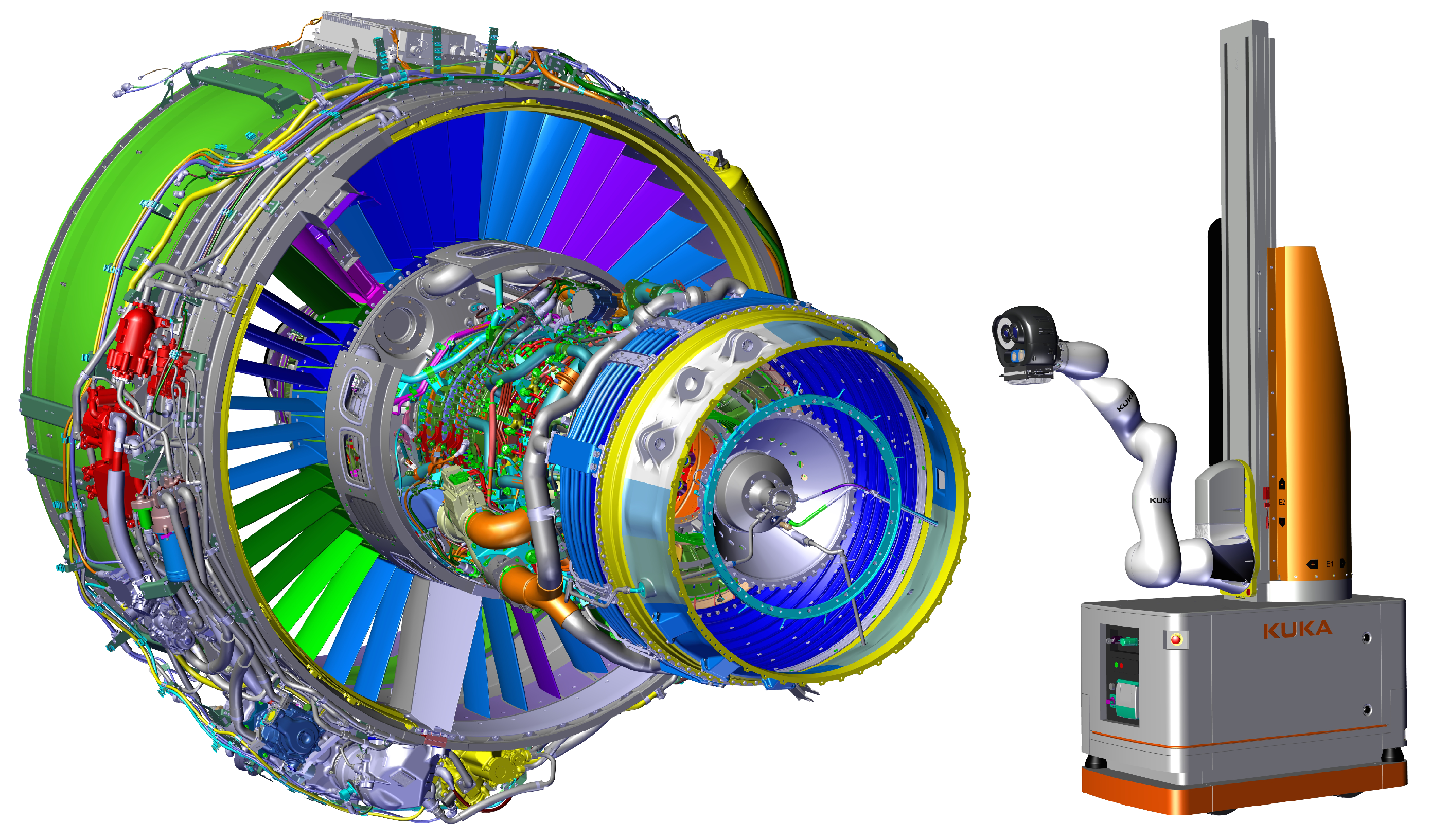
Figure 1.
The robot-based inspection platform and an aircraft engine to be inspected.
Figure 1.
The robot-based inspection platform and an aircraft engine to be inspected.
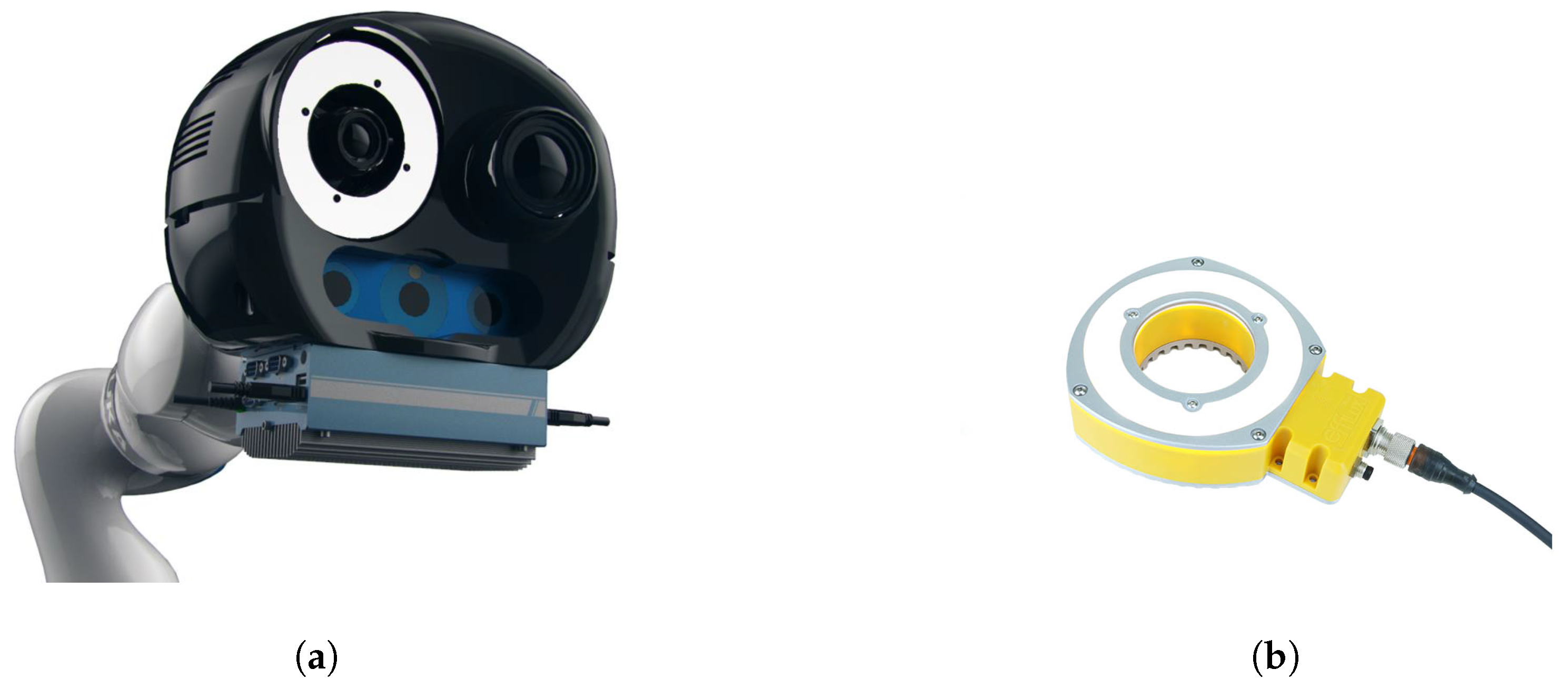
Figure 2.
(a) Vision-based sensory system mounted on the robot; (b) additional lighting around the inspection camera.
Figure 2.
(a) Vision-based sensory system mounted on the robot; (b) additional lighting around the inspection camera.
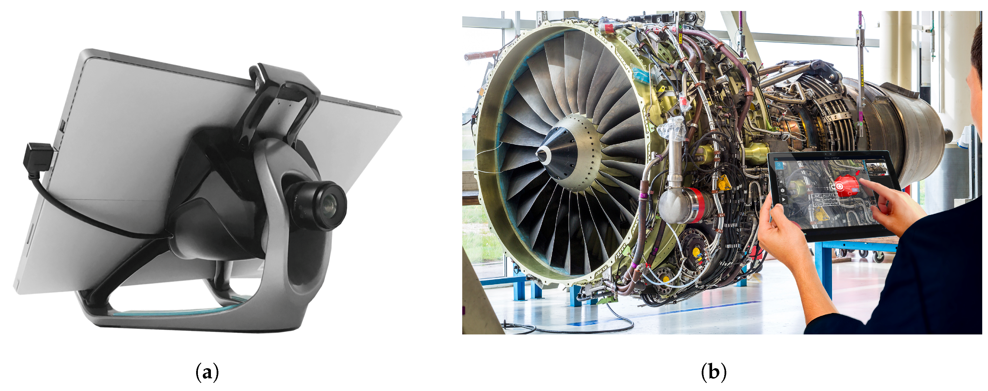
Figure 3.
Tablet-based interface equipped with a camera for visual inspection. (a) the tablet-based interface equipped with a camera (b) the tablet-based handheld interface used by an operator for the inspection of an aircraft engine
Figure 3.
Tablet-based interface equipped with a camera for visual inspection. (a) the tablet-based interface equipped with a camera (b) the tablet-based handheld interface used by an operator for the inspection of an aircraft engine
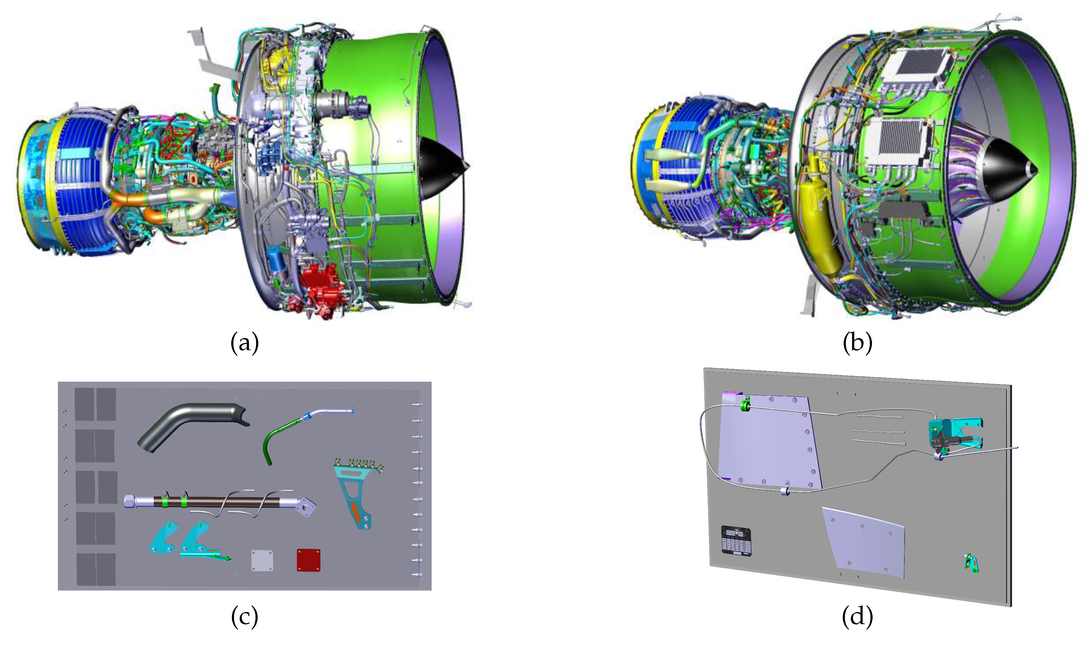
Figure 4.
Some of our CAD models: (a,b) aircraft engine, (c,d) two testing plates with several elements.
Figure 4.
Some of our CAD models: (a,b) aircraft engine, (c,d) two testing plates with several elements.
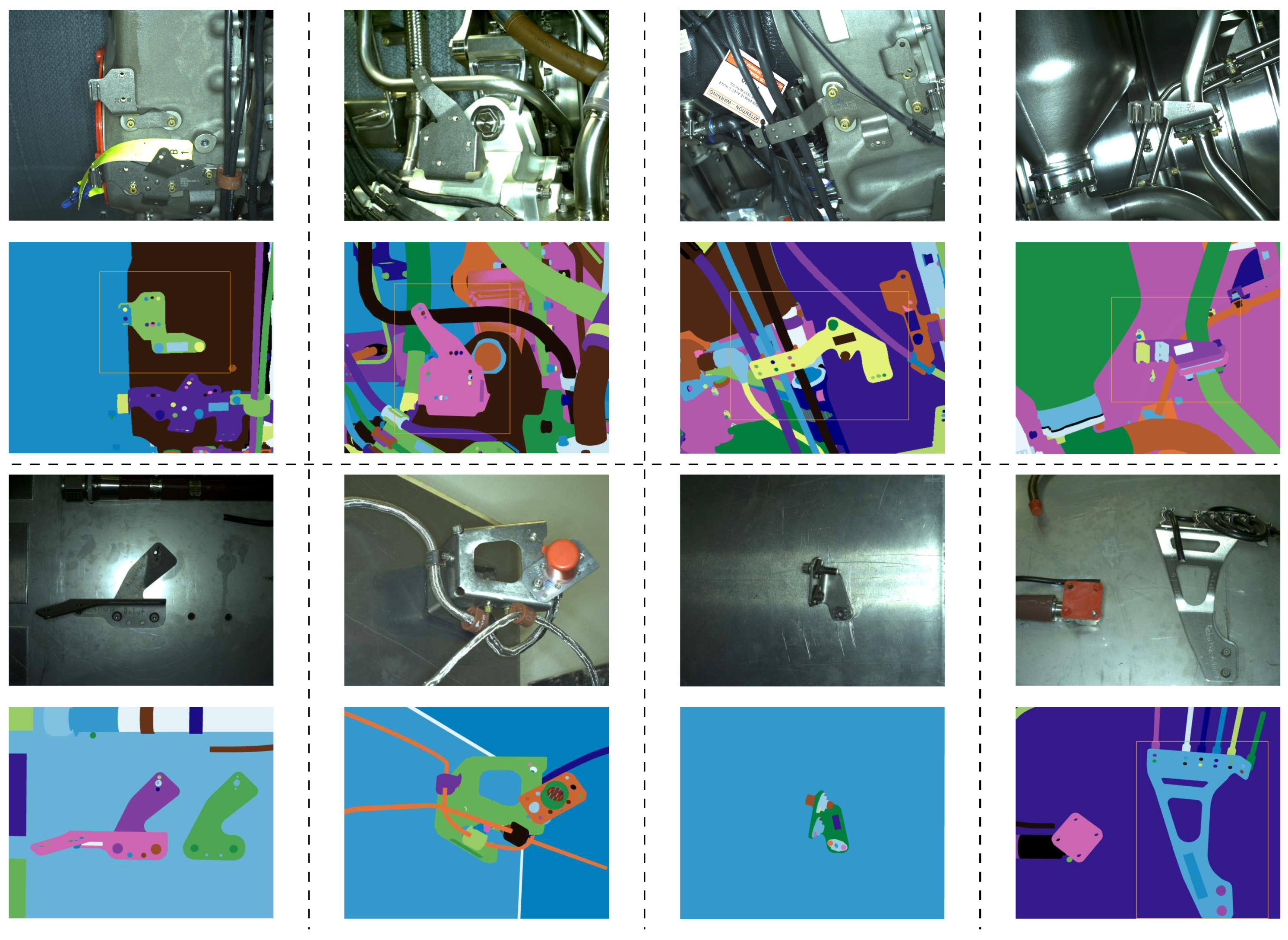
Figure 5.
Examples of our dataset: (1st and 3rd rows) real images and (2nd and 4th rows) corresponding renders of CAD models.
Figure 5.
Examples of our dataset: (1st and 3rd rows) real images and (2nd and 4th rows) corresponding renders of CAD models.
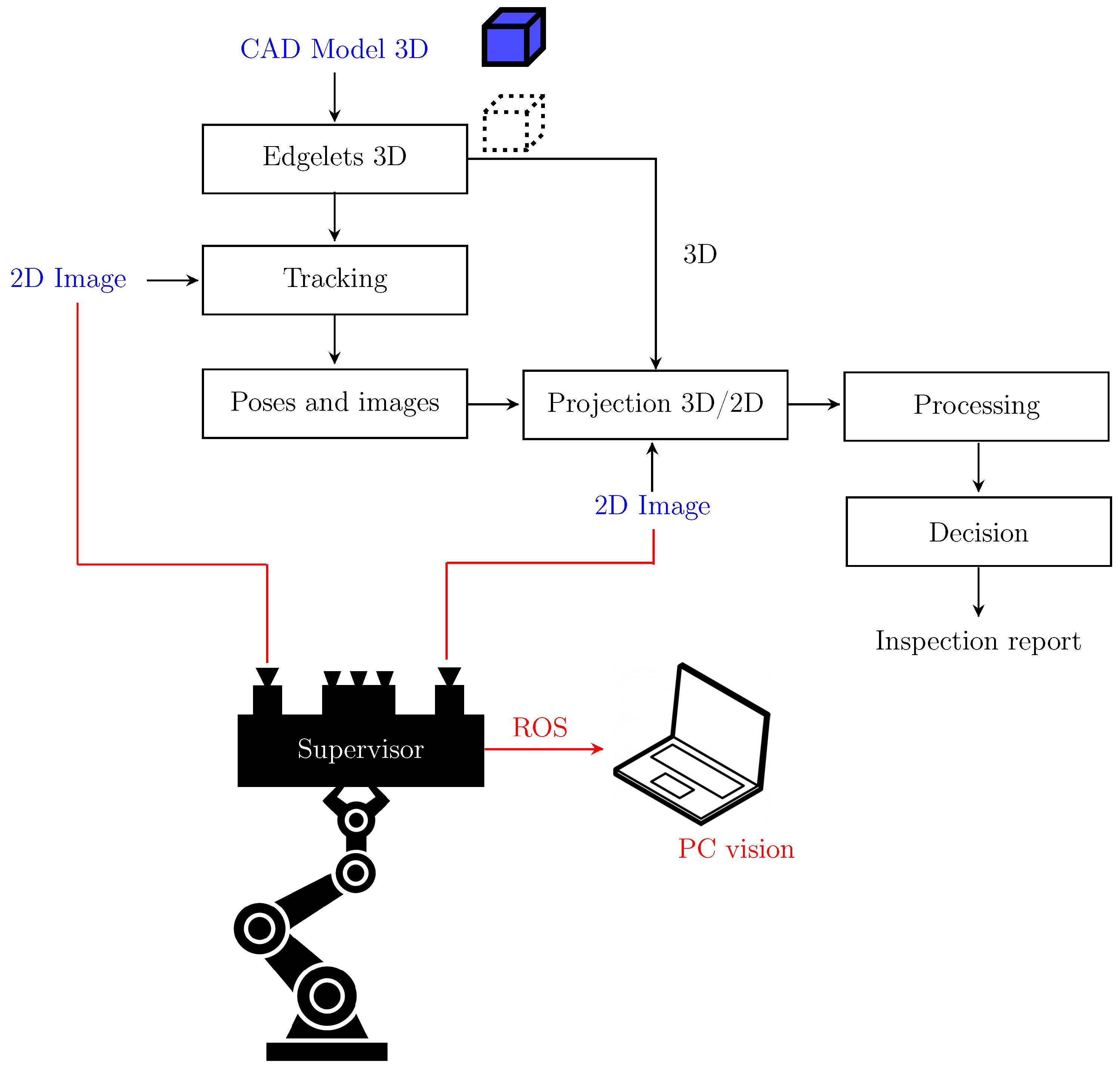
Figure 6.
Overview of the detection phase during online processing using robot-based inspection.
Figure 6.
Overview of the detection phase during online processing using robot-based inspection.
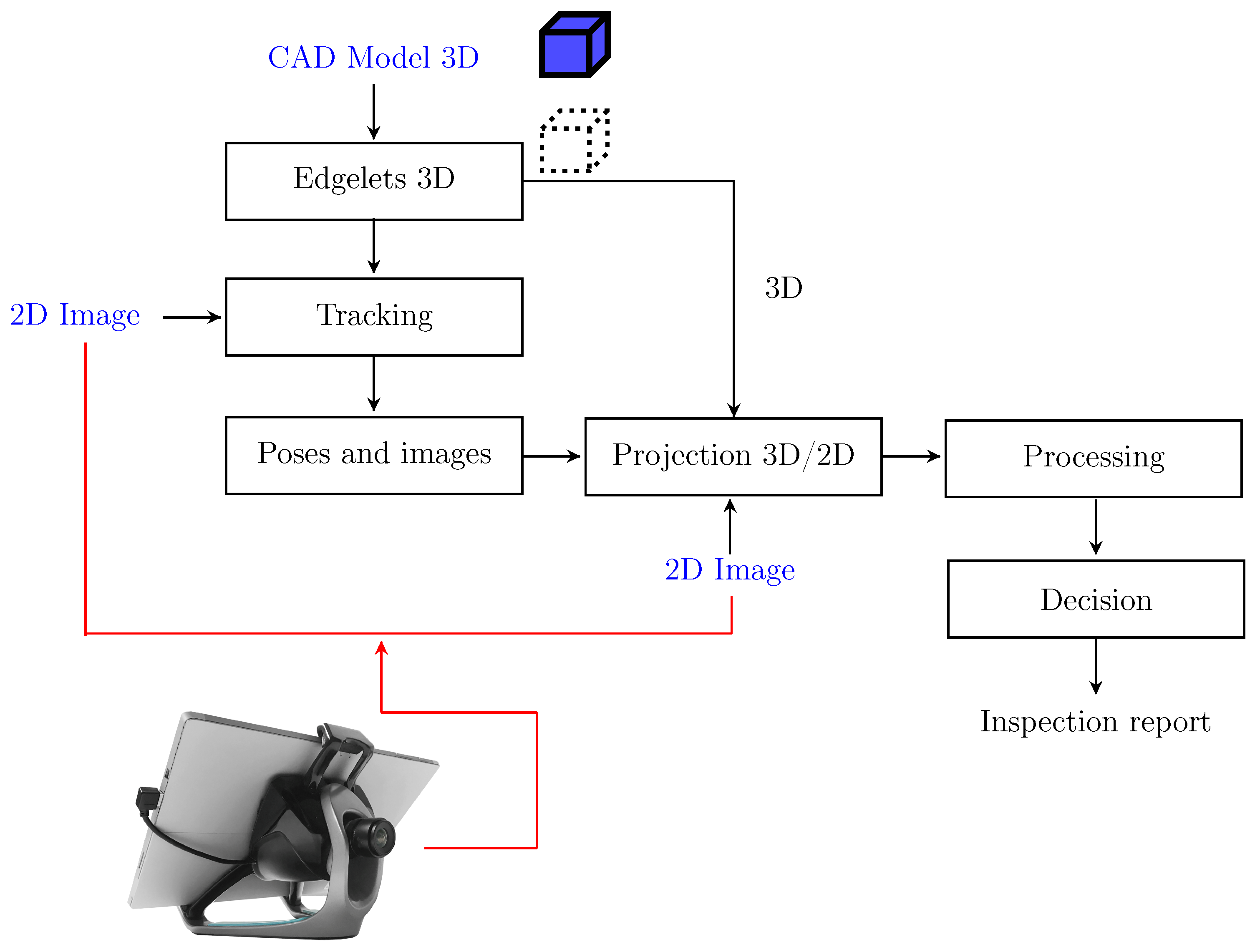
Figure 7.
Overview of the detection phase during online processing using tablet-based inspection.
Figure 7.
Overview of the detection phase during online processing using tablet-based inspection.
Figure 8.
Edgelets extraction: (a) example of CAD part, and (b) edgelets extracted from this CAD part.
Figure 8.
Edgelets extraction: (a) example of CAD part, and (b) edgelets extracted from this CAD part.
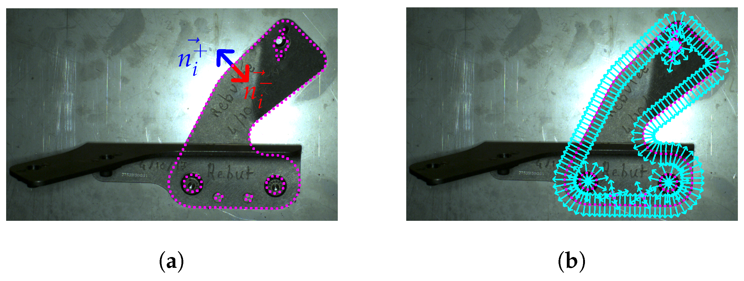
Figure 9.
(a) Projection of edgelets (3D points ), and (b) inward-pointing normals, , outward-pointing normals, , and generation of search line .
Figure 9.
(a) Projection of edgelets (3D points ), and (b) inward-pointing normals, , outward-pointing normals, , and generation of search line .
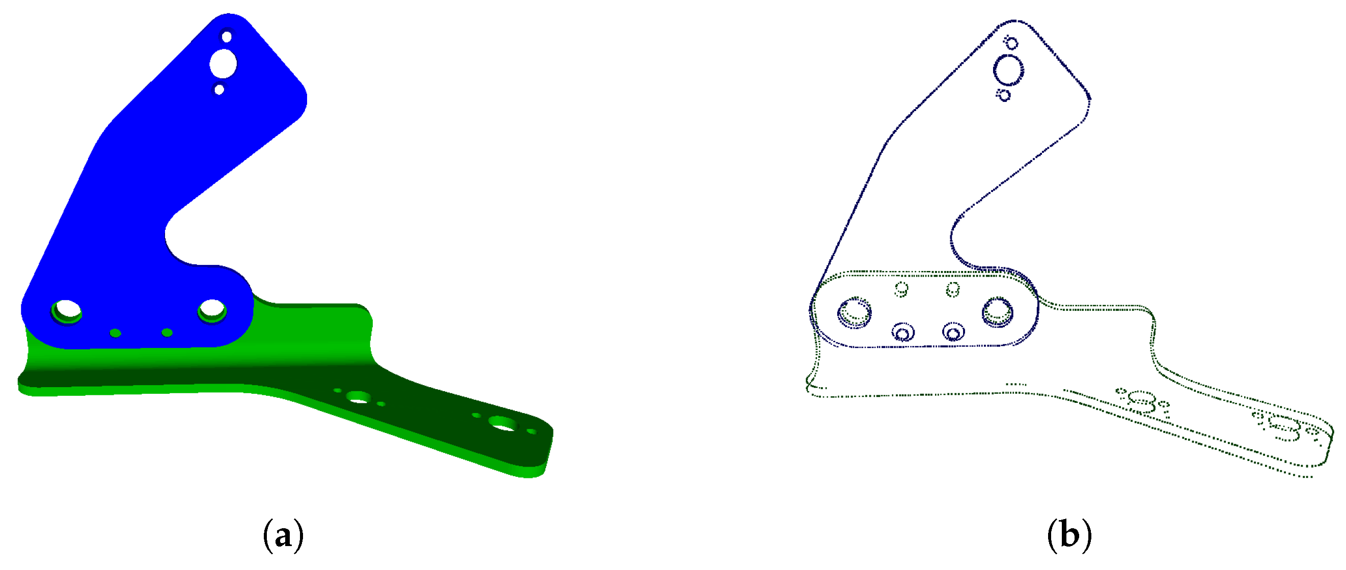
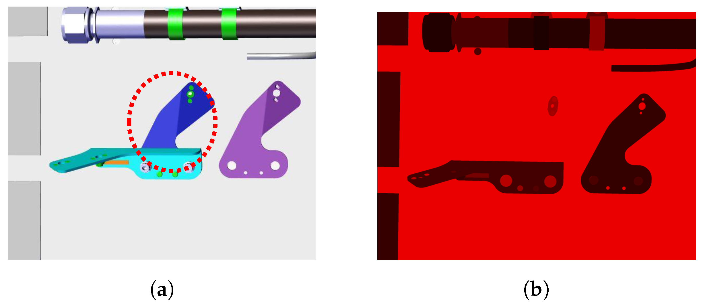
Figure 10.
(a) Example of CAD model; (b) context image of the blue element.
Figure 10.
(a) Example of CAD model; (b) context image of the blue element.
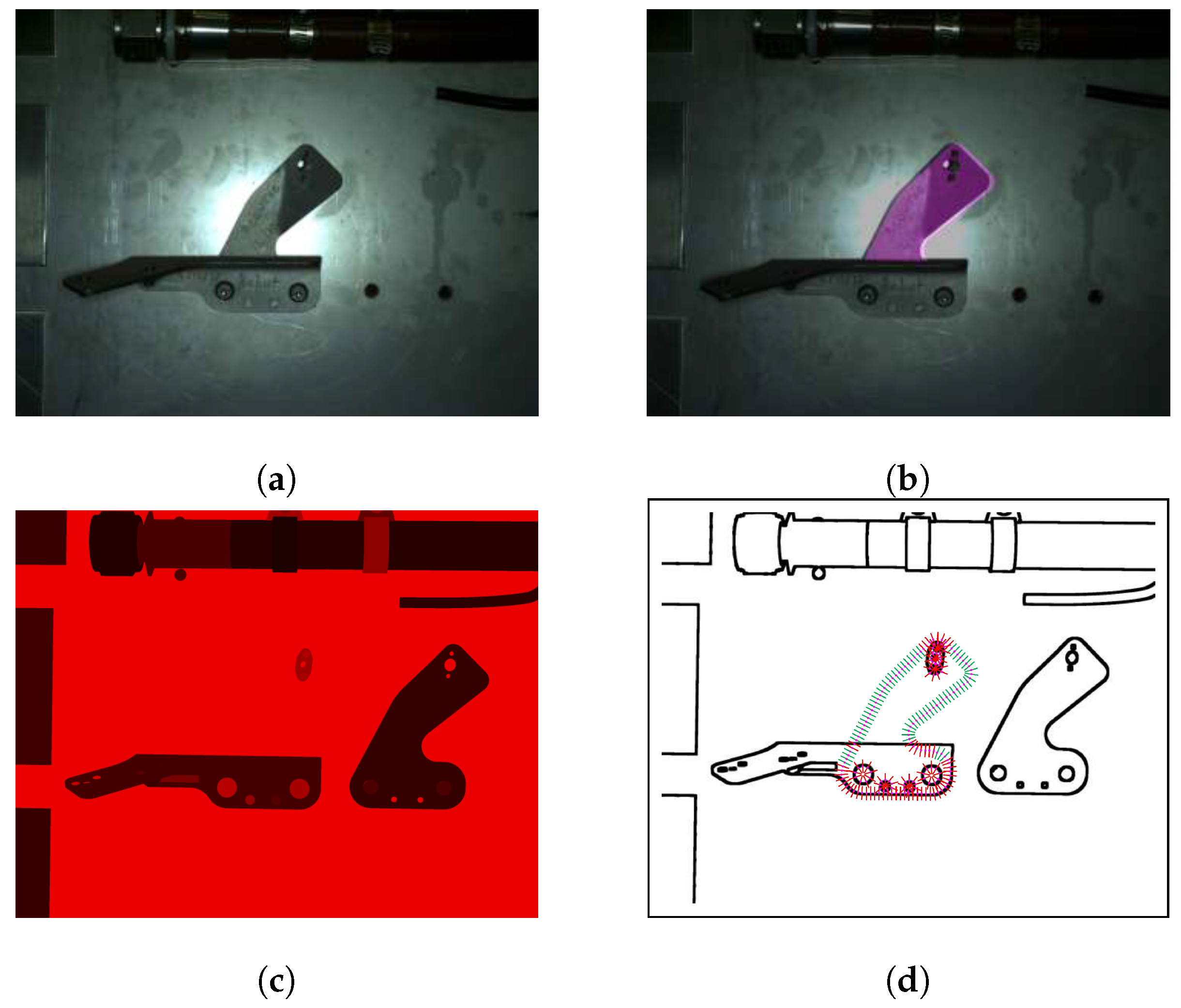
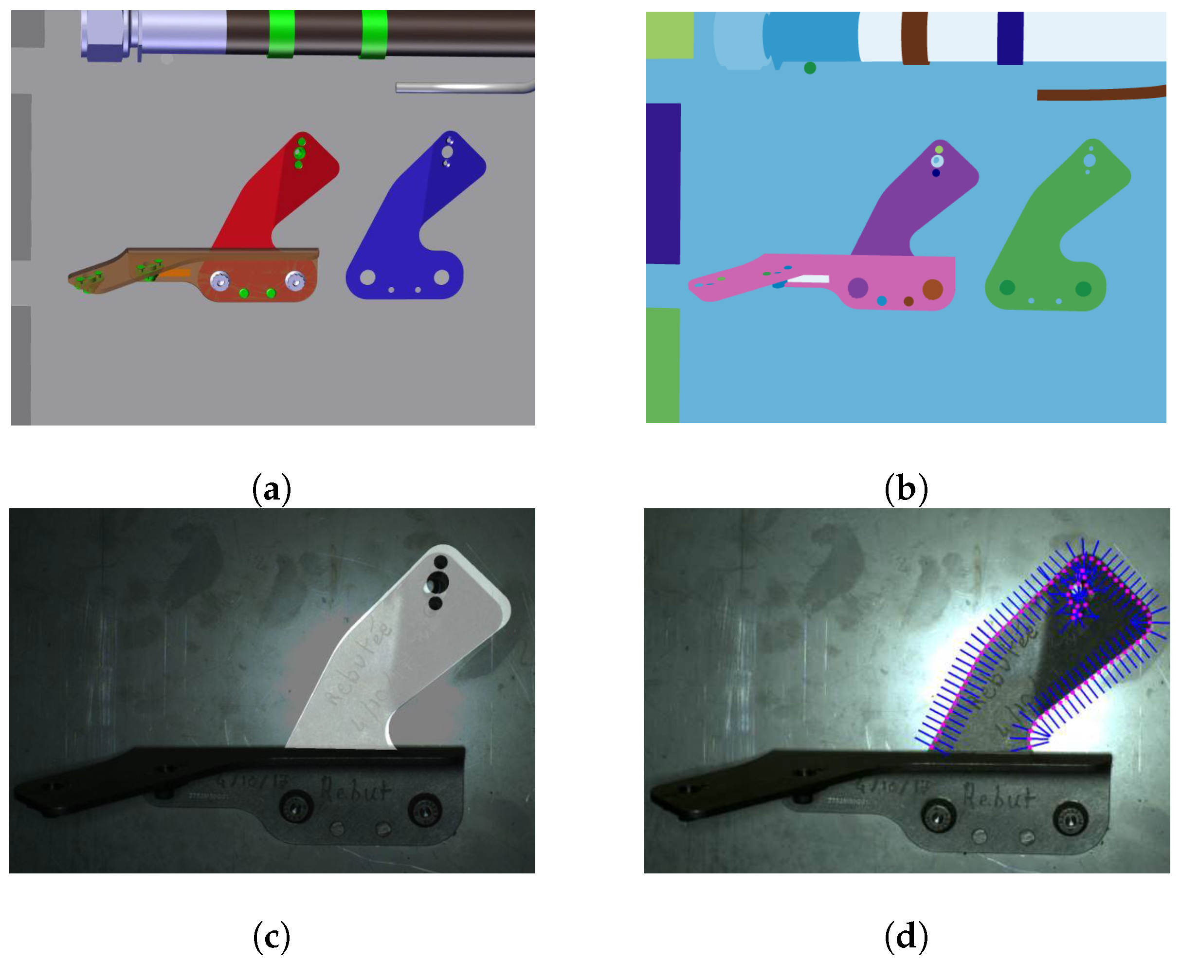
Figure 11.
Illustration of the parasitic edges handling: (a) input image, (b) projection of the element to be inspected, (c) context image of the element to be inspected and its projected edgelets, and (d) gradient changes in the context image and considered edgelets (green) and rejected edgelets (red).
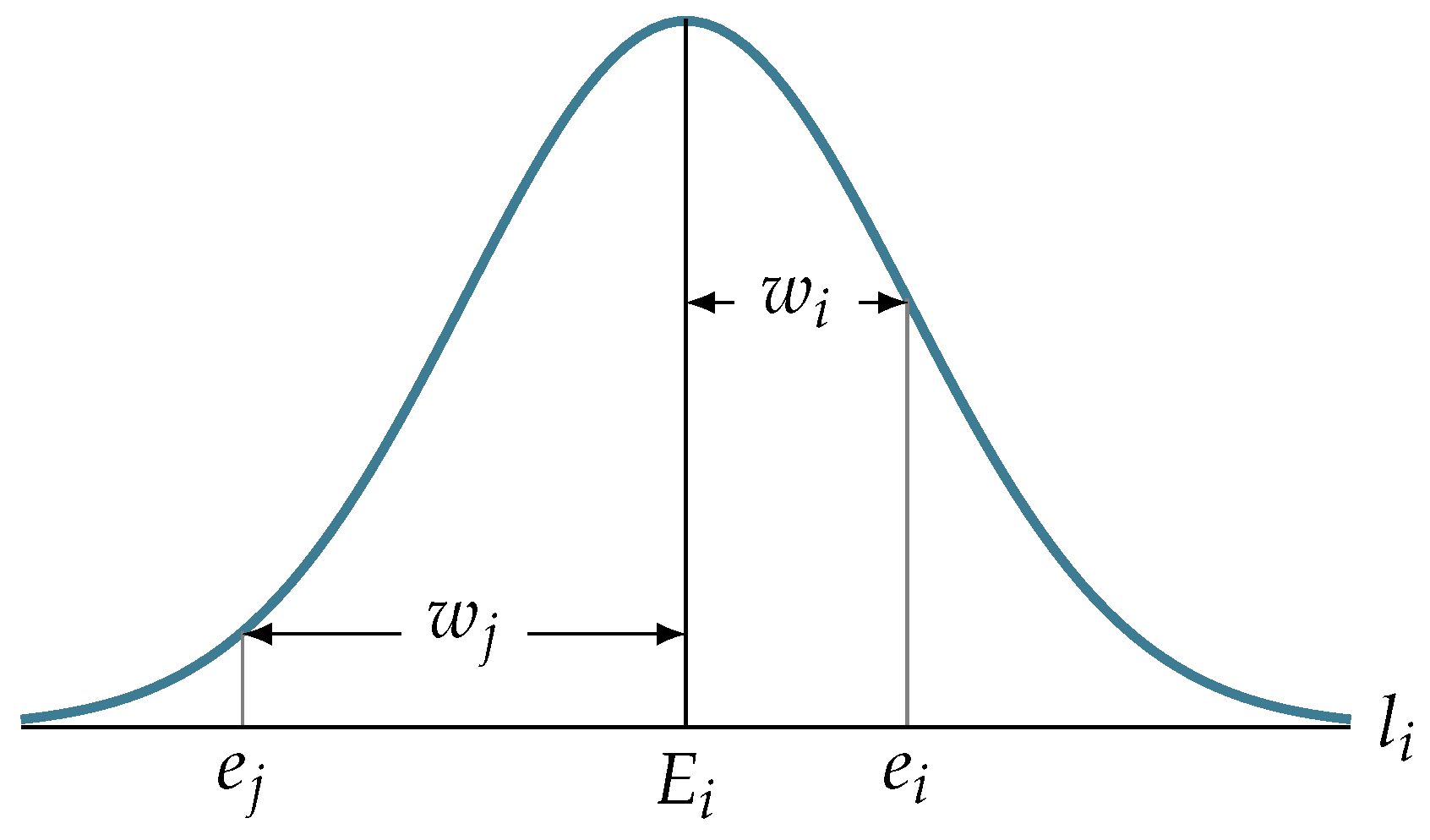
Figure 12.
Illustration of edges weighting.
Figure 12.
Illustration of edges weighting.
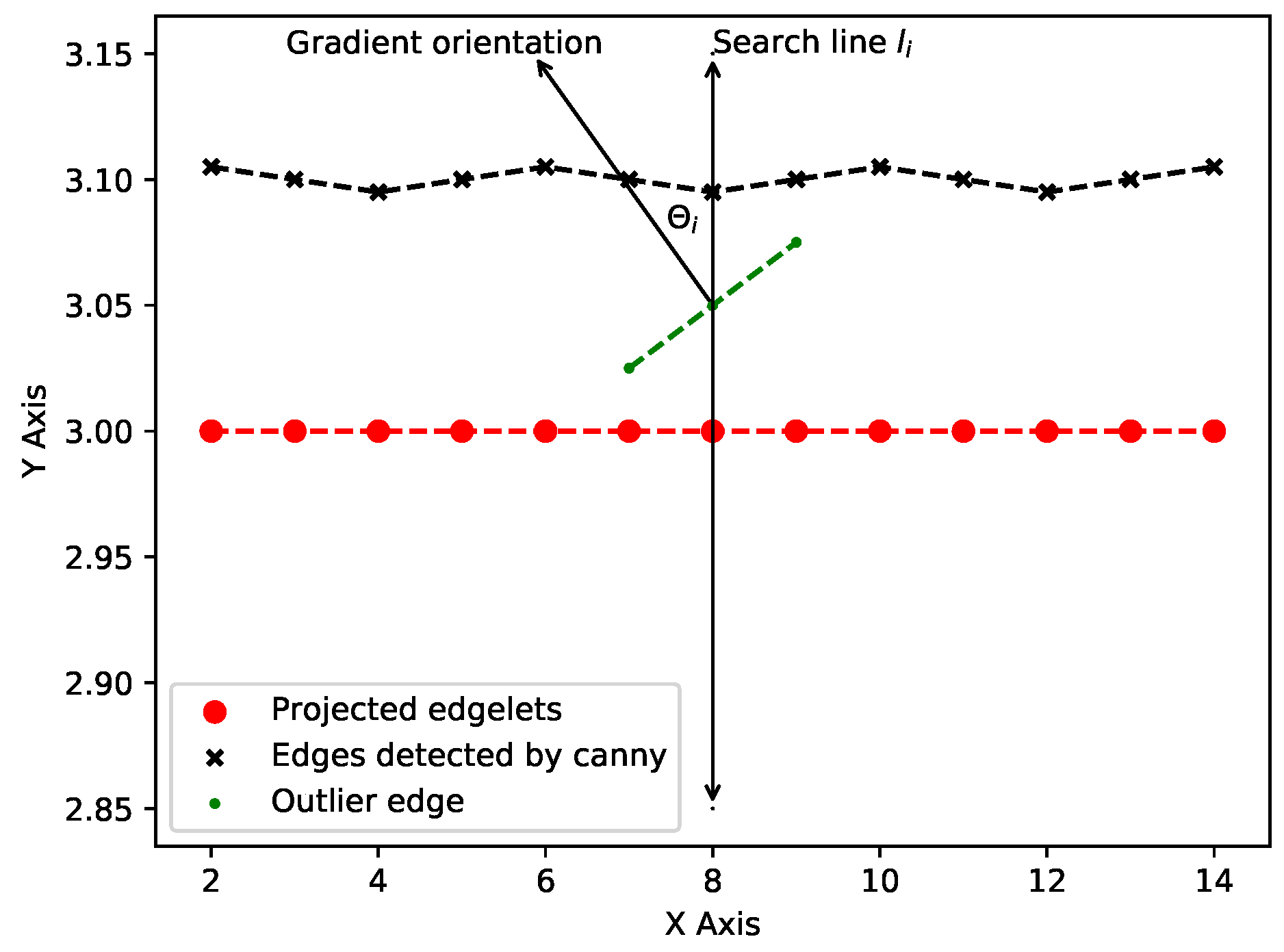
Figure 13.
Challenges due to outlier edges, such as those due to image noise and edges arising from features that do not belong to the inspection element, when searching for an image edge corresponding to the projected edgelet.
Figure 13.
Challenges due to outlier edges, such as those due to image noise and edges arising from features that do not belong to the inspection element, when searching for an image edge corresponding to the projected edgelet.
Figure 14.
Occlusion handling by rendering using Color Rendering Index (CRI): (
a) CAD model rendered with CATIA composer, (
b) CAD model rendered using CRI, (
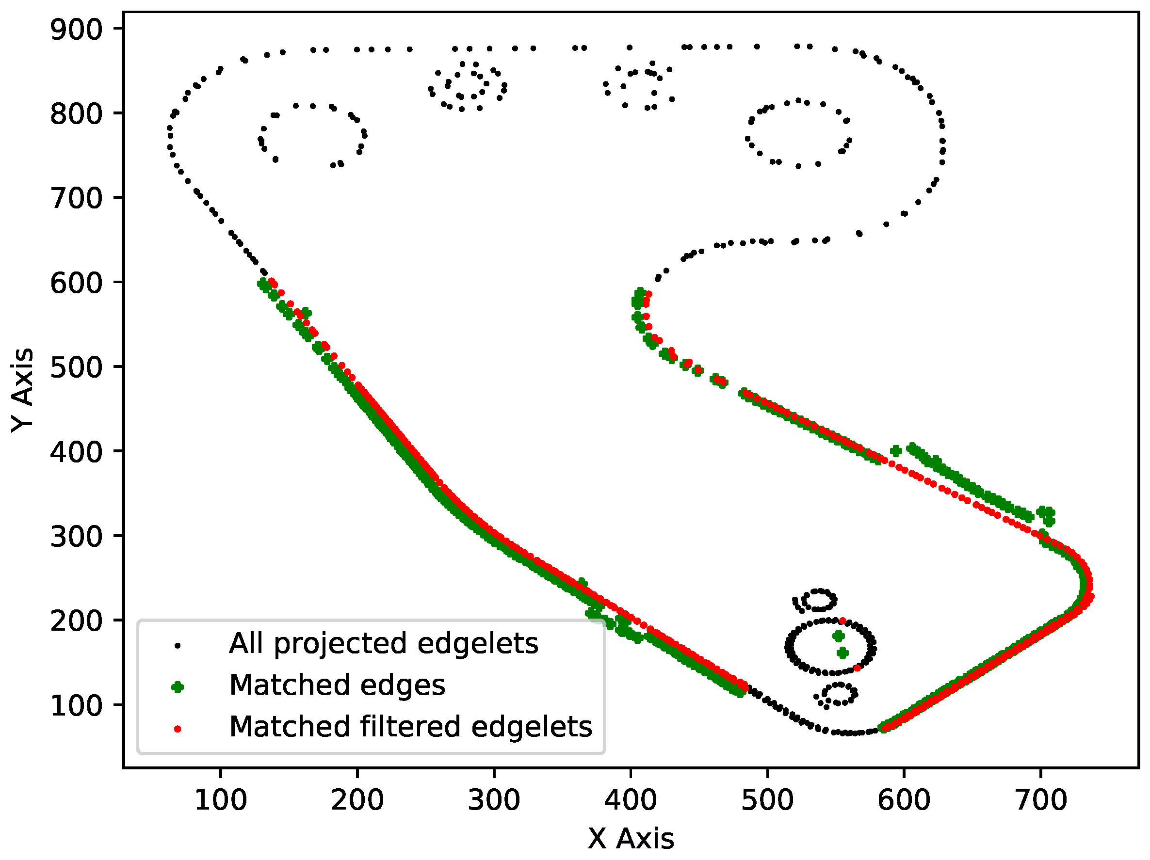
c) mask generated using CRI render, white areas represent region to be inspected, and (
d) filtered edgelets (
Figure 11d) projected inside the region of interest specified by the generated mask.
Figure 14.
Occlusion handling by rendering using Color Rendering Index (CRI): (
a) CAD model rendered with CATIA composer, (
b) CAD model rendered using CRI, (
c) mask generated using CRI render, white areas represent region to be inspected, and (
d) filtered edgelets (
Figure 11d) projected inside the region of interest specified by the generated mask.
Figure 15.
The shapes used in the shape context approach.
Figure 15.
The shapes used in the shape context approach.
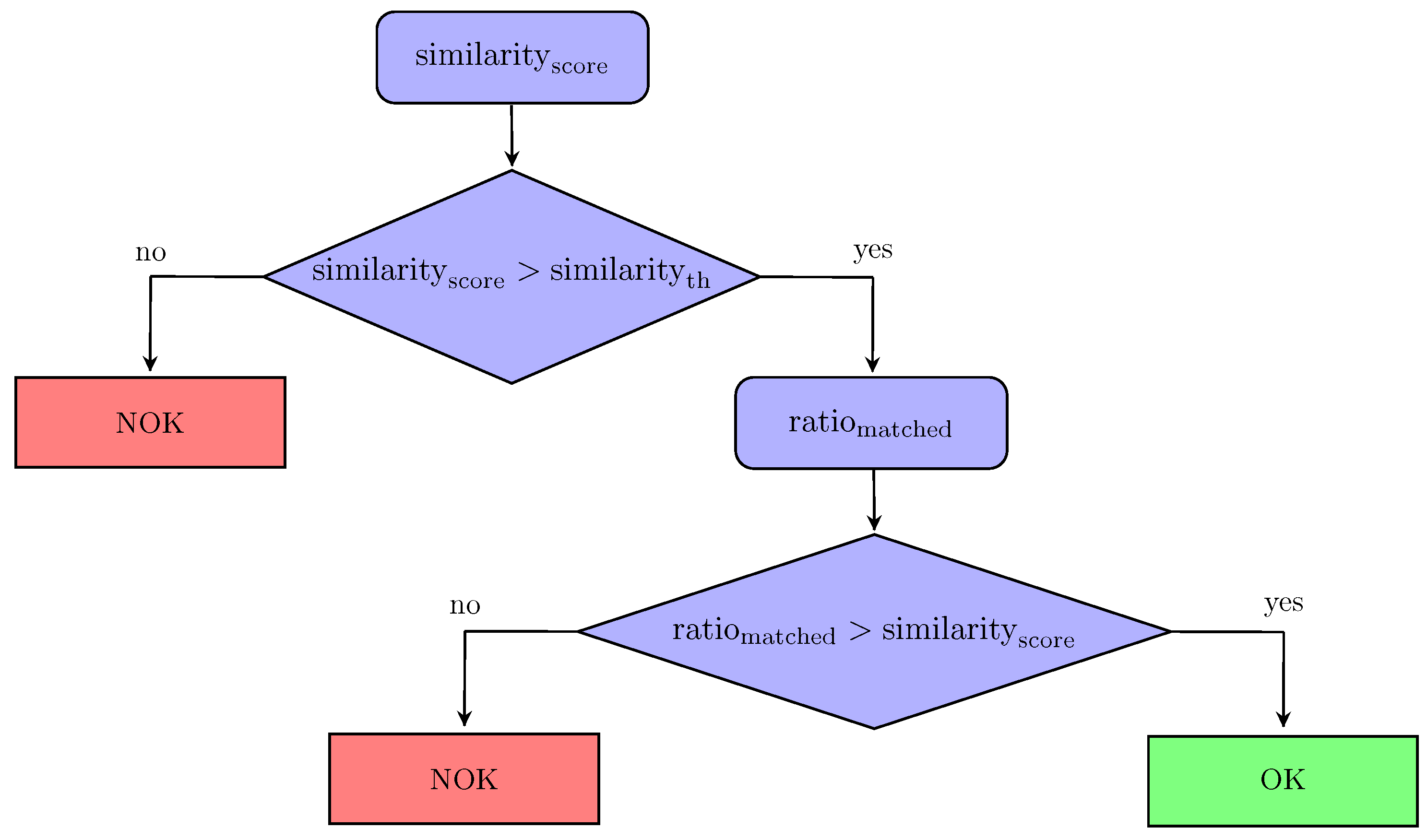
Figure 16.
Decision-making.
Figure 16.
Decision-making.
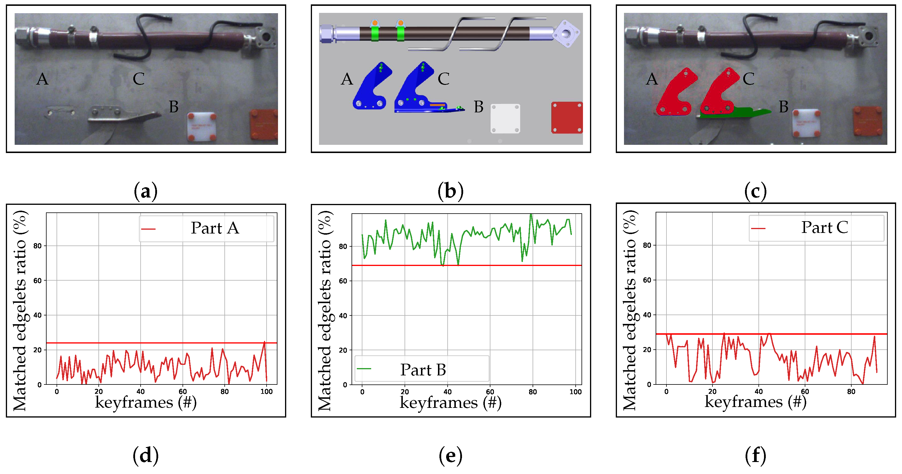
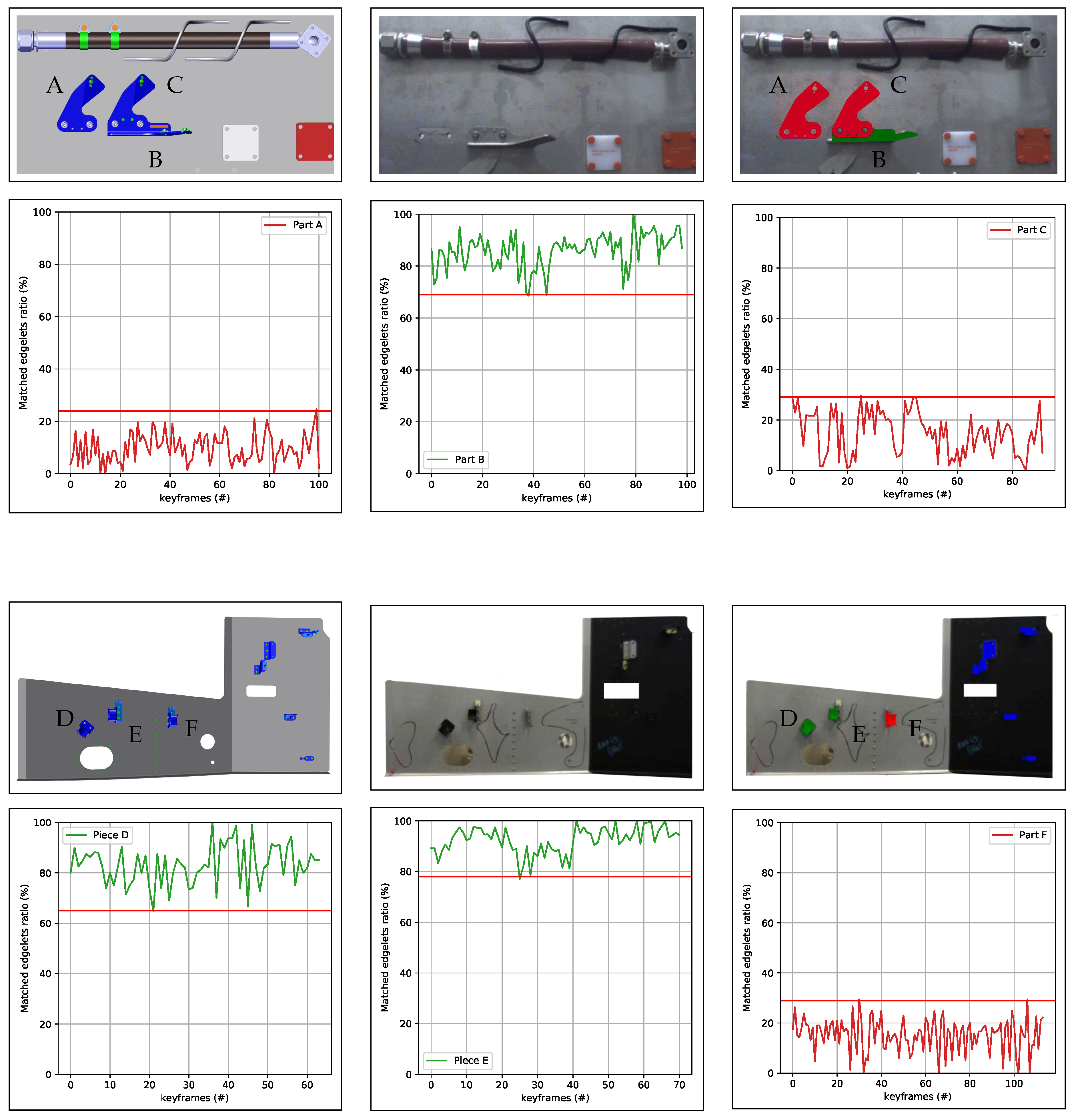
Figure 17.
(a) CAD model; (b) input image; (c) result of inspection with green OK (element present) and red NOK (element absent or incorrectly mounted); (d–f) the (curve) and threshold (red horizontal line), respectively, computed on the three different cases: element A (absent) in red, element B (present) in green, and element C (incorrectly mounted) in red.
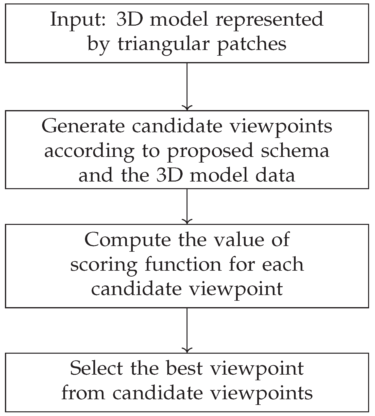
Figure 18.
The overview of viewpoint selection scheme.
Figure 18.
The overview of viewpoint selection scheme.
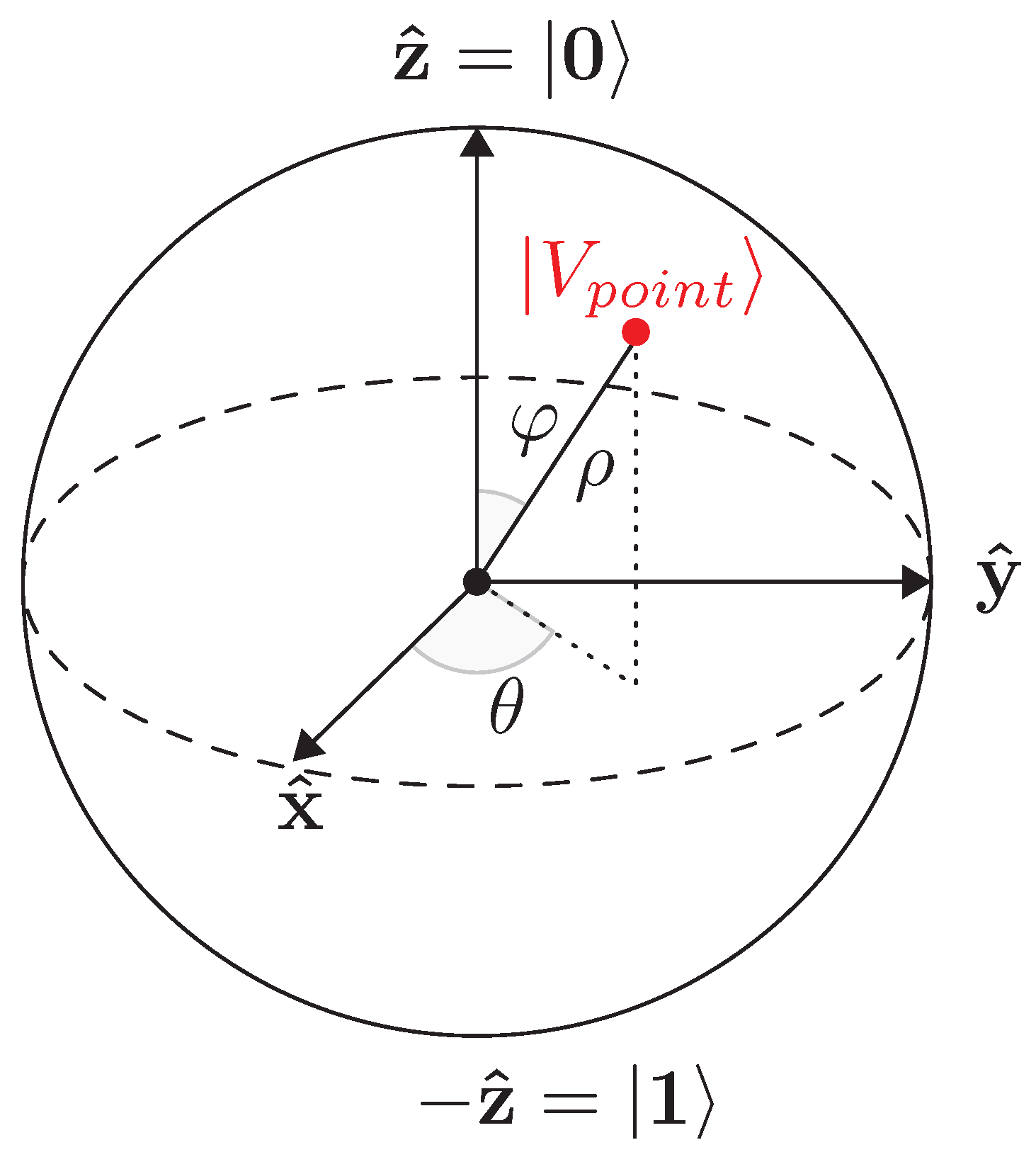
Figure 19.
A viewpoint on the visibility sphere.
Figure 19.
A viewpoint on the visibility sphere.
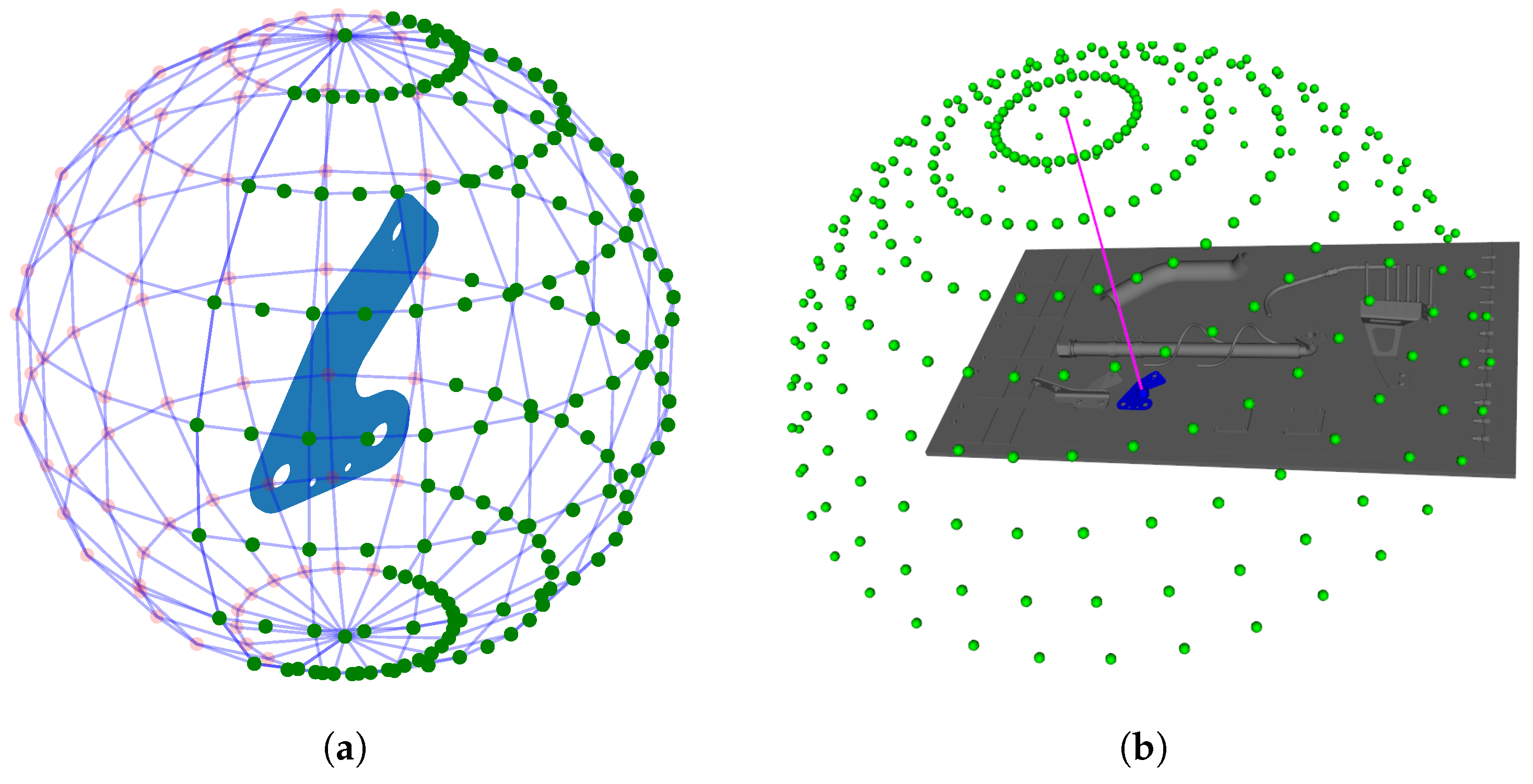
Figure 20.
The candidate viewpoint region is defined as a part of sphere surface. The accessible viewpoints in green and the inaccessible viewpoints, due to occlusions related to the global CAD, in red (a) for a given element to be inspected and (b) for the whole assembly.
Figure 20.
The candidate viewpoint region is defined as a part of sphere surface. The accessible viewpoints in green and the inaccessible viewpoints, due to occlusions related to the global CAD, in red (a) for a given element to be inspected and (b) for the whole assembly.
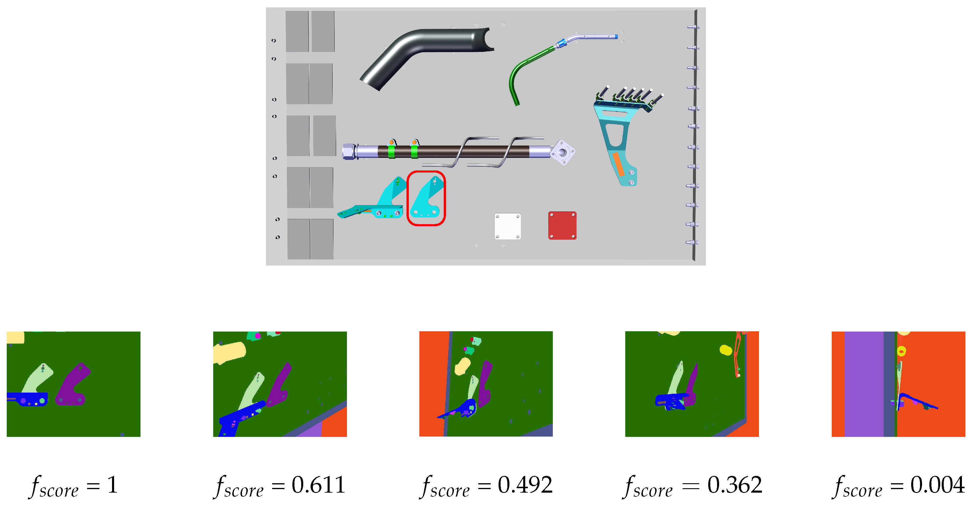
Figure 21.
(1st row) CAD model and (2nd row) different candidate viewpoints for inspecting the element in the red rectangle, with the corresponding .
Figure 21.
(1st row) CAD model and (2nd row) different candidate viewpoints for inspecting the element in the red rectangle, with the corresponding .
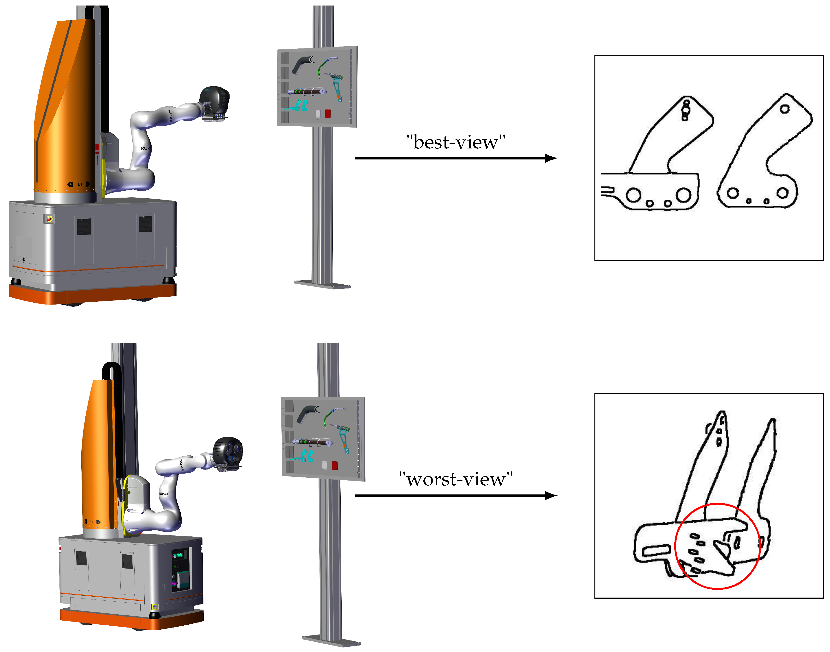
Figure 22.
Two viewpoints with best-view and worst-view according to the number of parasite edges.
Figure 22.
Two viewpoints with best-view and worst-view according to the number of parasite edges.
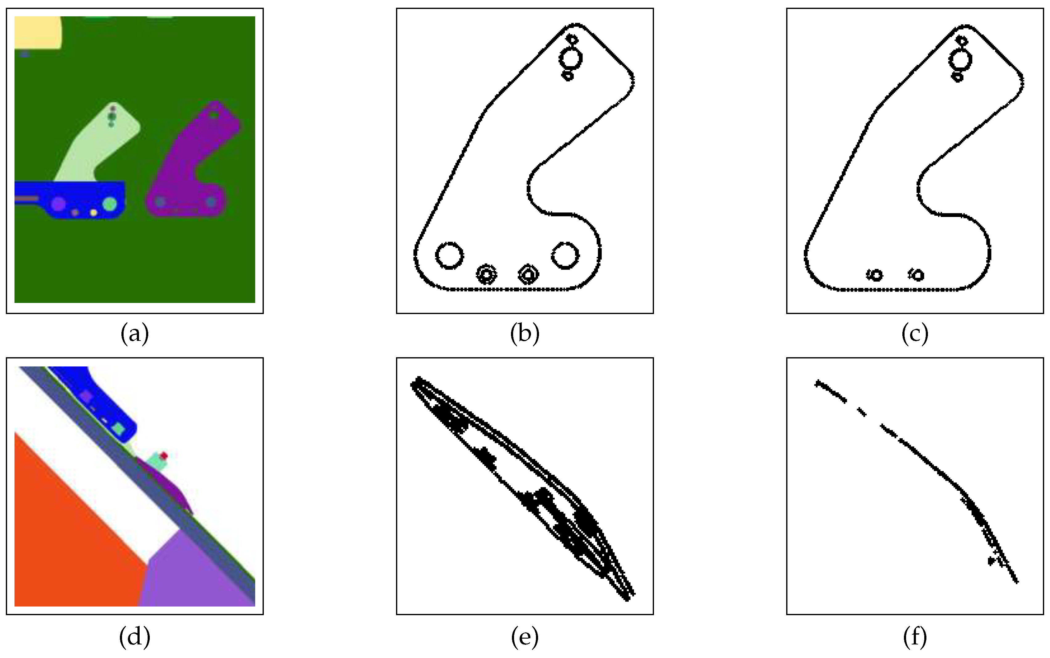
Figure 23.
(a) “Best-view”, (b) all edgelets of best-view, (c) filtred edgelets of best-view, (d) “worst-view”, (e) all edgelets of worst-view, and (f) filtered edgelets of worst-view.
Figure 23.
(a) “Best-view”, (b) all edgelets of best-view, (c) filtred edgelets of best-view, (d) “worst-view”, (e) all edgelets of worst-view, and (f) filtered edgelets of worst-view.
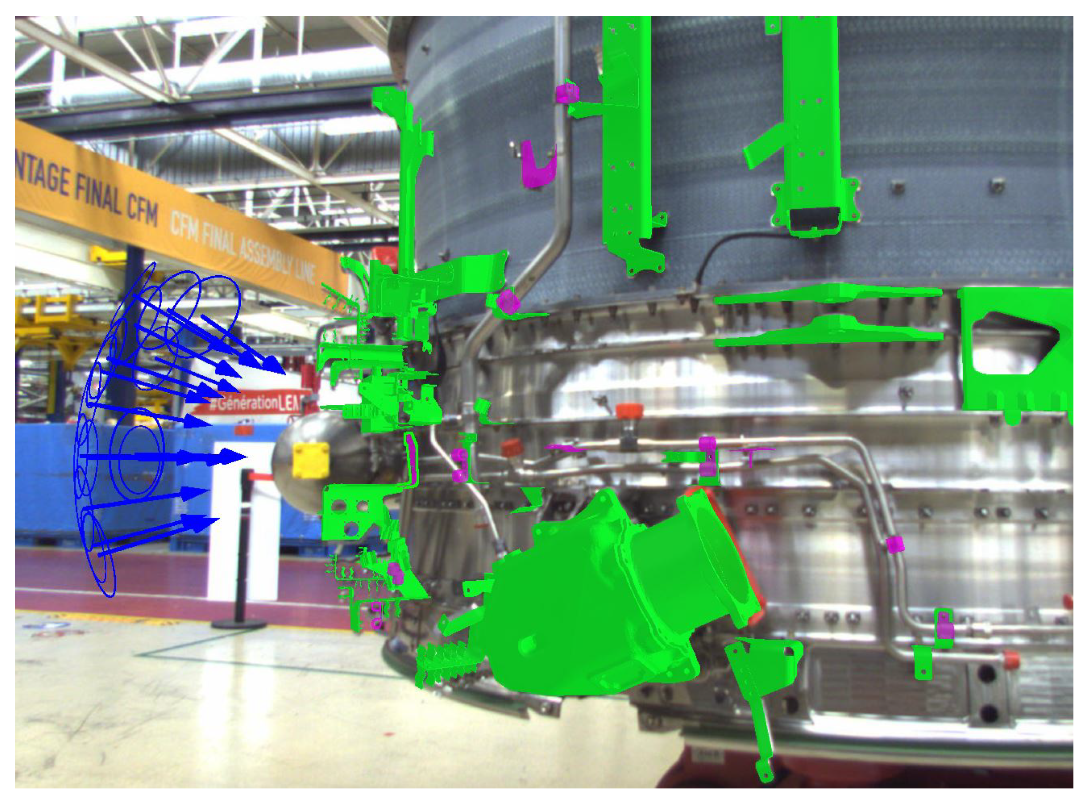
Figure 24.
User guidance in the handheld tablet mode (see the blue arrows).
Figure 24.
User guidance in the handheld tablet mode (see the blue arrows).
Figure 25.
Experimental results for determining the optimal . The red horizontal line represents the min matched ratio in the case OK (element in green) and the max matched ratio in the case NOK (element in red).
Figure 25.
Experimental results for determining the optimal . The red horizontal line represents the min matched ratio in the case OK (element in green) and the max matched ratio in the case NOK (element in red).
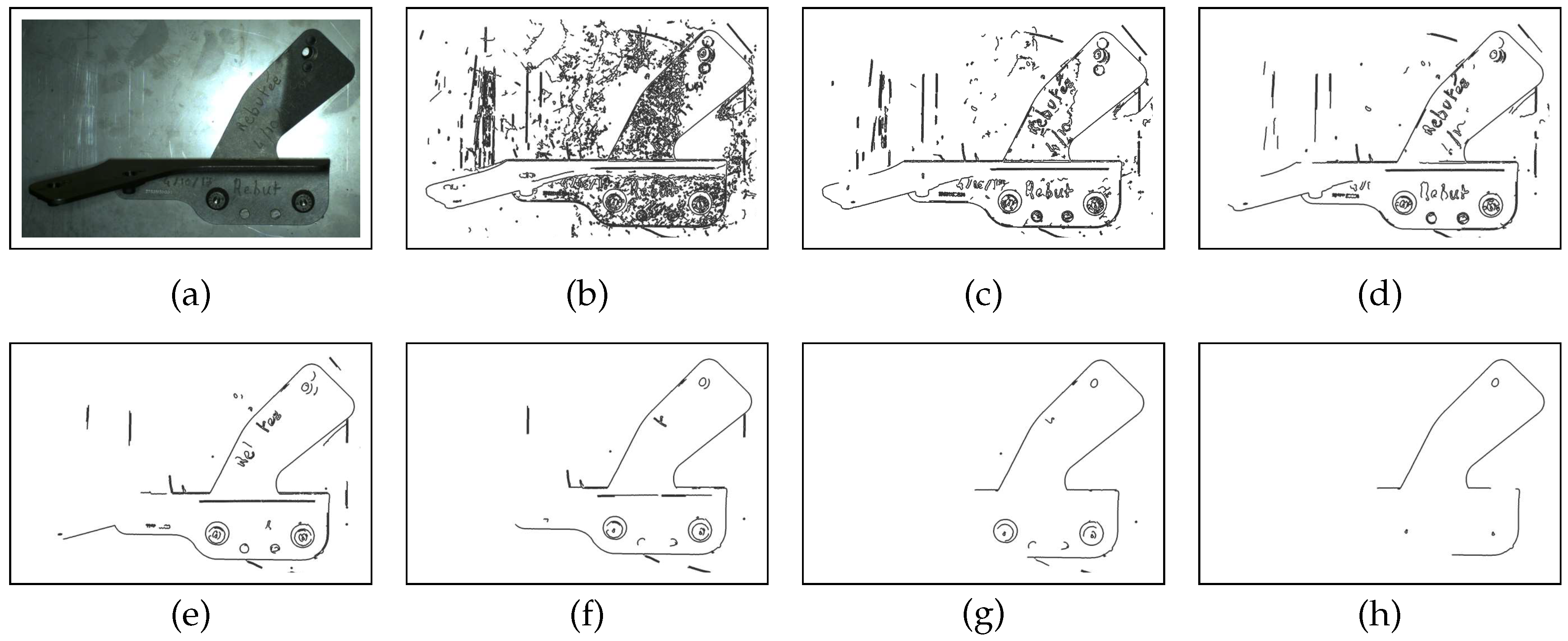
Figure 26.
Images of Canny algorithm results (
a). Images (
b–
h) have been obtained using the high and low threshold values specified in
Table 4.
Figure 26.
Images of Canny algorithm results (
a). Images (
b–
h) have been obtained using the high and low threshold values specified in
Table 4.
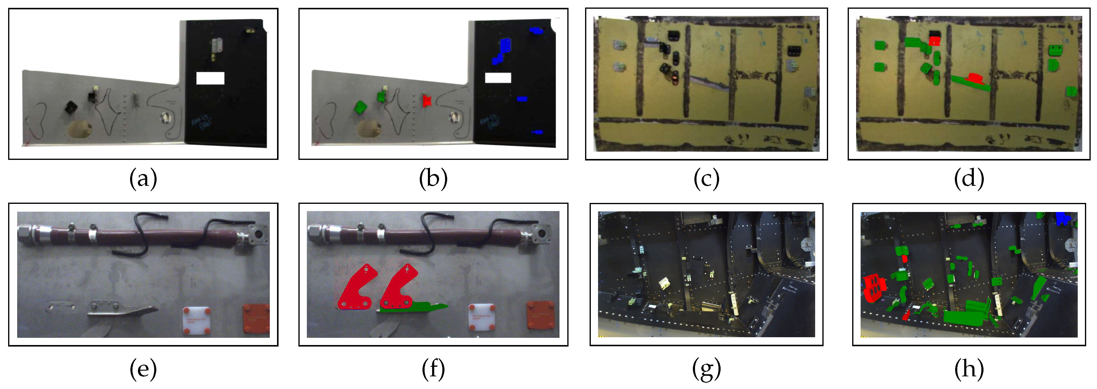
Figure 27.
Dataset used to evaluate our algorithms: (a,c,e,g) real images and (b,d,f,h) corresponding inspection results with OK elements in green and NOK elements in red.
Figure 27.
Dataset used to evaluate our algorithms: (a,c,e,g) real images and (b,d,f,h) corresponding inspection results with OK elements in green and NOK elements in red.
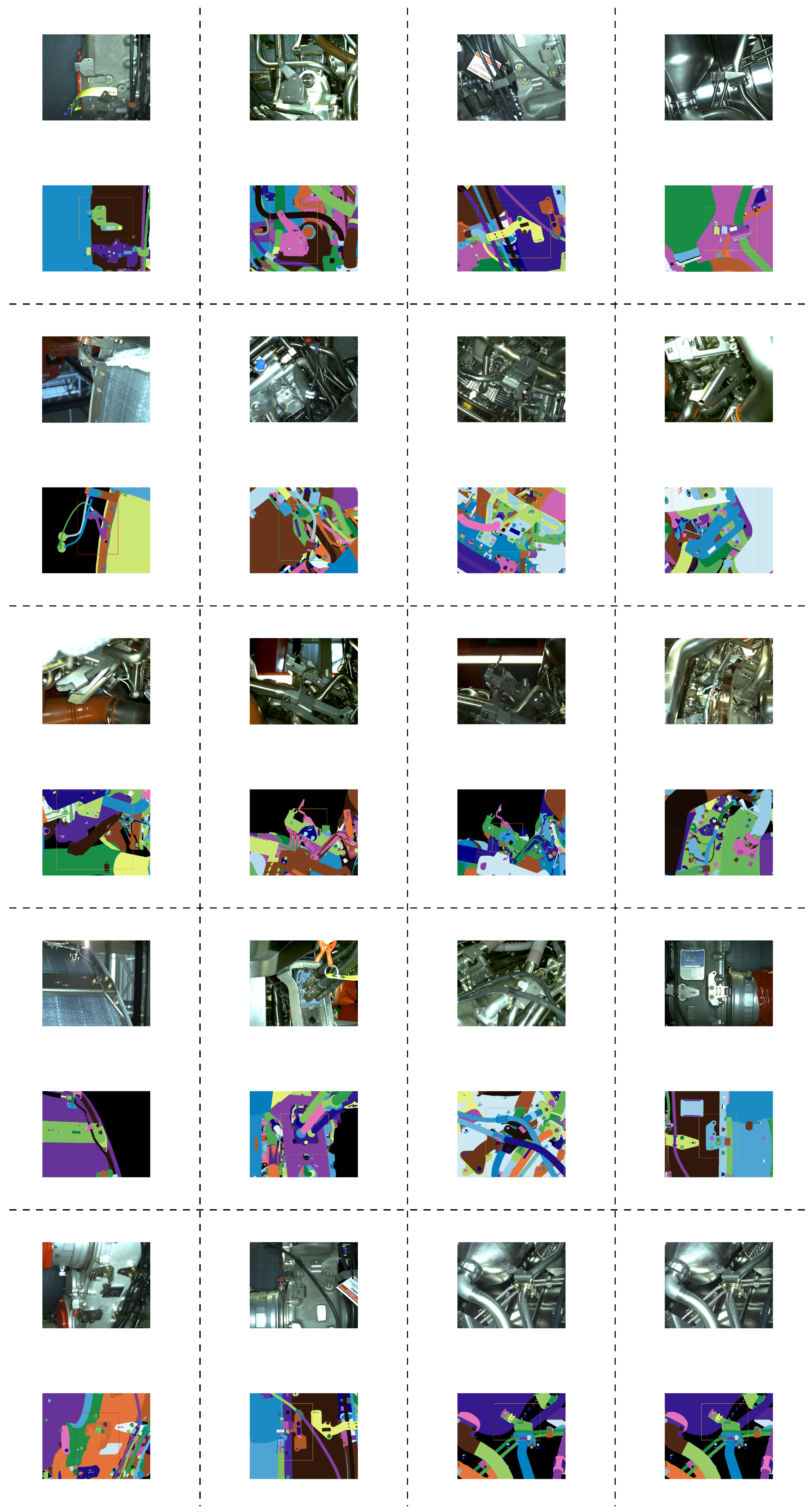
Figure 28.
Some examples of our dataset used to evaluate our approach in a context of robotized inspection in conditions of very cluttered environment.
Figure 28.
Some examples of our dataset used to evaluate our approach in a context of robotized inspection in conditions of very cluttered environment.
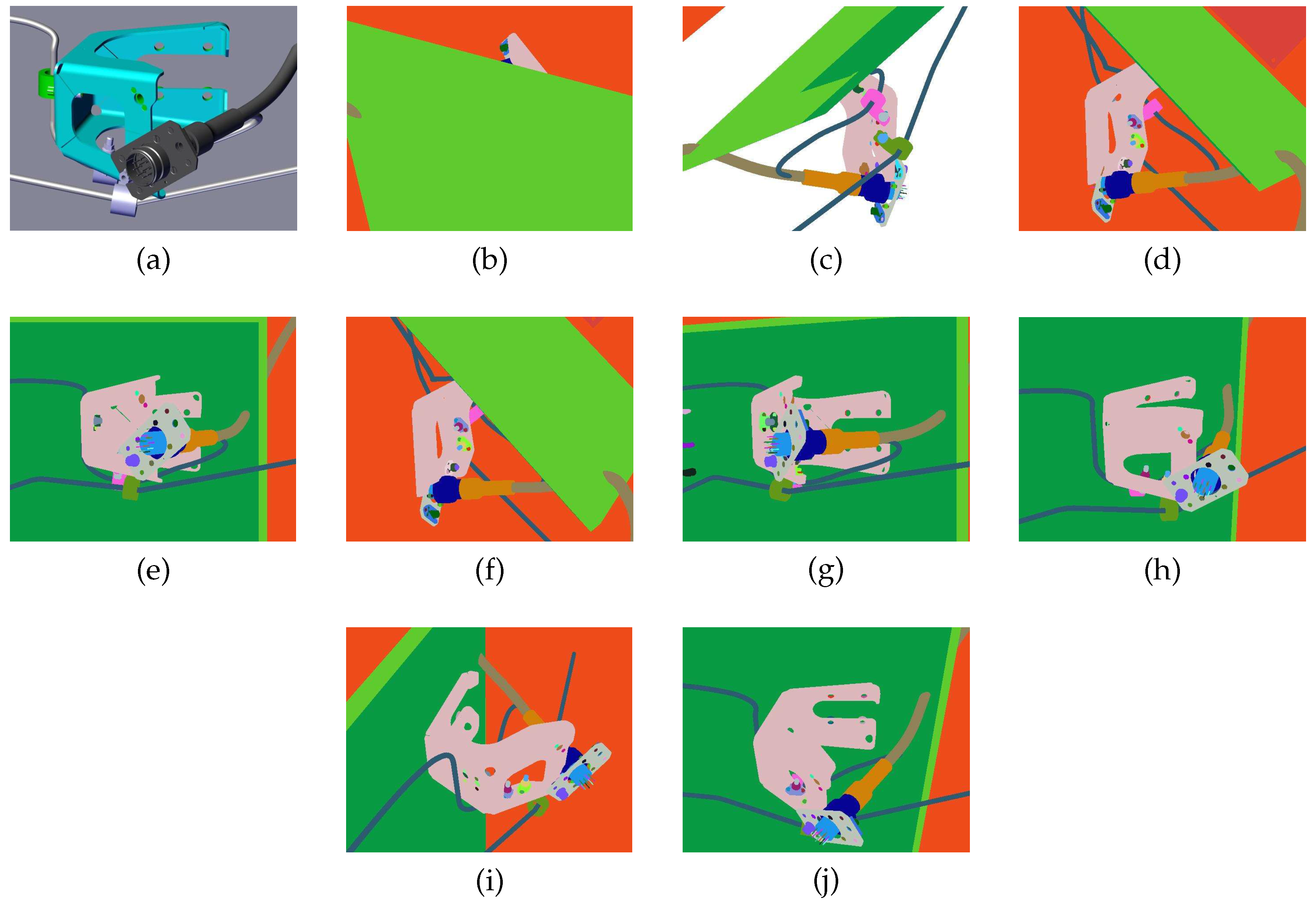
Figure 29.
Images (
b–
j) correspond to different viewpoints of the element shown on image (
a). The
of each viewpoint is provided in
Table 10.
Figure 29.
Images (
b–
j) correspond to different viewpoints of the element shown on image (
a). The
of each viewpoint is provided in
Table 10.
Table 1.
Inspection camera specifications.
Table 1.
Inspection camera specifications.
| Camera name | UI-3180 (PYTHON 5000) |
|---|
| Frame rate | 73 fps |
| Resolution () | |
| Optical Area | mm × 9.830 mm |
| Resolution | MPix |
| Pixel size | 4.80 m |
| Lens name | vs- |
| Focal length | 25 mm () |
| Minimal object distance (M.O.D.) | 300 mm |
| Angel of view () | |
Table 2.
Tracking camera specifications.
Table 2.
Tracking camera specifications.
| Camera name | IDS 3070 |
|---|
| Frame rate | 123 fps |
| Resolution () | |
| Optical Area | 7.093 mm × 5.0320 mm |
| Resolution | MPix |
| Pixel size | 3.45 m |
| Lens name | Kowa 8 mm |
| Focal length | 8 mm |
| Minimal object distance (M.O.D.) | mm |
| Angel of view () | |
Table 3.
Determination of optimal parameter for making decision on state of element.
Table 3.
Determination of optimal parameter for making decision on state of element.
| Inspecting Element | State of Element | Max Matched Edgelet Ratio | Min Matched Edgelet Ratio |
|---|
| Part A | NOK | 25% | 0% |
| Part B | OK | 100% | 68% |
| Part C | NOK | 30% | 0% |
| Part D | OK | 100% | 70% |
| Part E | OK | 100% | 65% |
| Part F | NOK | 25% | 0% |
Table 4.
The proportional coefficient of high and low thresholds of Canny algorithm in
Figure 26a.
Table 4.
The proportional coefficient of high and low thresholds of Canny algorithm in
Figure 26a.
Table 5.
Definitions of TP, FP, TN, and FN in defect detection.
Table 5.
Definitions of TP, FP, TN, and FN in defect detection.
| | Actually Defective | Actually Non-Defective |
|---|
| Detected as defective | TP | FP |
| Detected as nondefective | FN | TN |
Table 6.
Result of the evaluation (TP, TN, FP, and FN).
Table 6.
Result of the evaluation (TP, TN, FP, and FN).
| Experiment | Number of Elements | Number of Images | TP | TN | FP | FN |
|---|
| 1 (Figure 27a,b) | 3 | 249 | 114 | 135 | 0 | 0 |
| 2 (Figure 27c,d) | 16 | 1580 | 305 | 1264 | 11 | 0 |
| 3 (Figure 27e,f) | 3 | 292 | 193 | 99 | 0 | 0 |
| 4 (Figure 27g,h) | 52 | 5135 | 607 | 4482 | 46 | 0 |
| Total | 74 | 7256 | 1219 | 5980 | 57 | 0 |
| Accuracy | Sensitivity | Specificity | Precision | Recall | |
|---|
| 99.12% | 100% | 99.01% | 95.53% | 100% | 97.71% |
Table 8.
Result of the evaluation (TP, TN, FP, and FN).
Table 8.
Result of the evaluation (TP, TN, FP, and FN).
| Number of Elements | Number of Images | TP | TN | FP | FN |
|---|
| 43 | 643 | 145 | 410 | 88 | 0 |
| Accuracy | Sensitivity | Specificity | Precision | Recall | |
|---|
| 86.31% | 100% | 82.32% | 62.23% | 100% | 76.72% |
Table 10.
The
of viewpoints for inspecting the element of
Figure 29a.
Table 10.
The
of viewpoints for inspecting the element of
Figure 29a.


