Color Image Complexity versus Over-Segmentation: A Preliminary Study on the Correlation between Complexity Measures and Number of Segments


Abstract
:1. Introduction
2. Materials and Methods
2.1. Image Data Bases
2.1.1. Color Fractal Images
2.1.2. Berkeley Segmentation Dataset
2.2. Color Image Complexity
2.2.1. Color Entropy
2.2.2. Color Fractal Dimension
2.3. Color Image Segmentation Approaches
2.3.1. Quasi-Flat Zones
2.3.2. JSEG
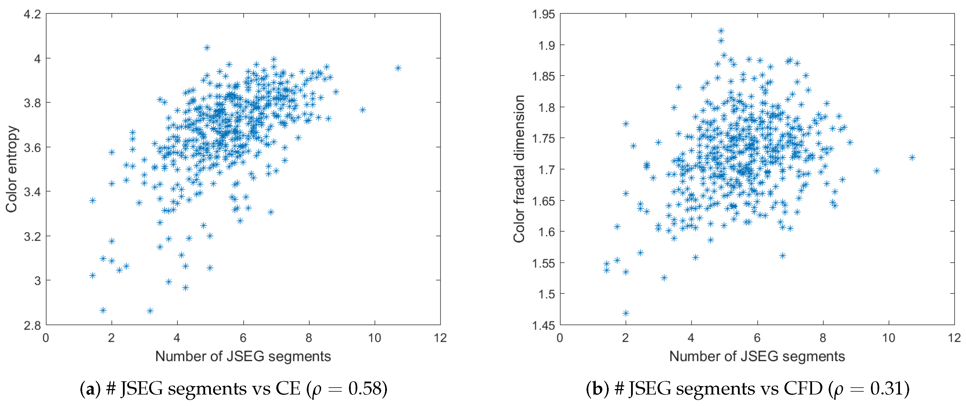
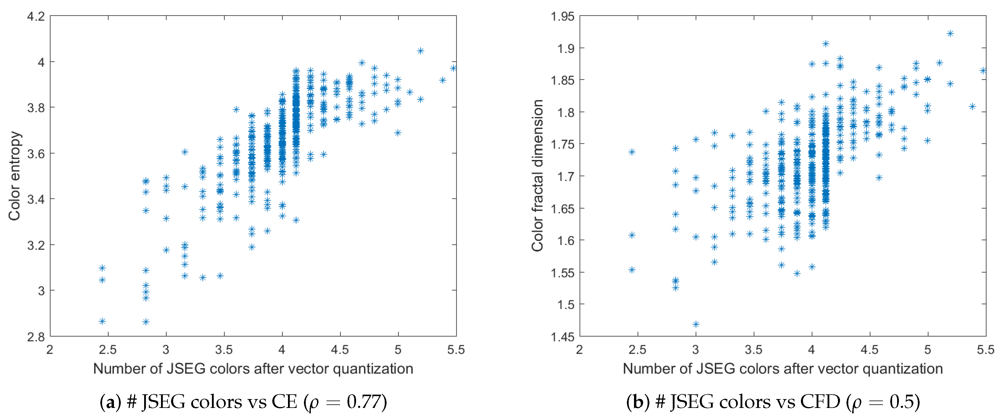
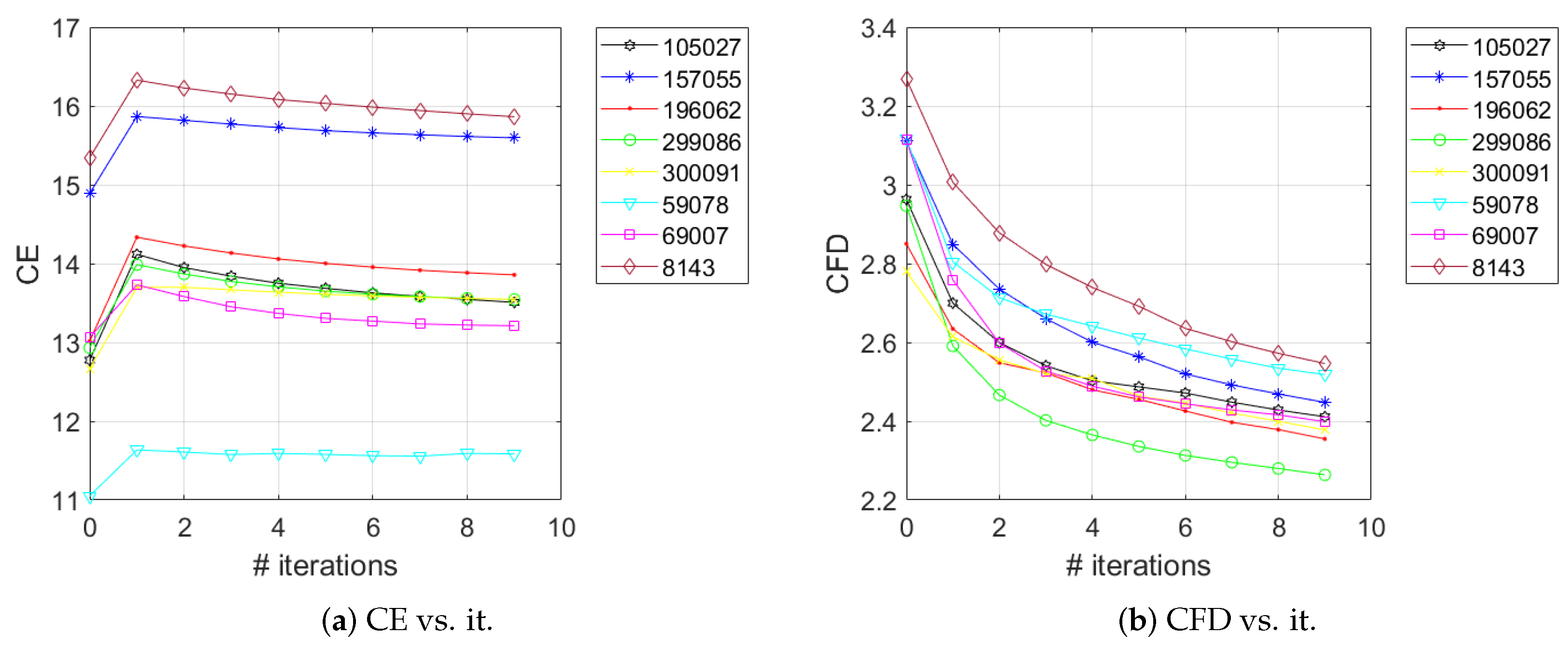
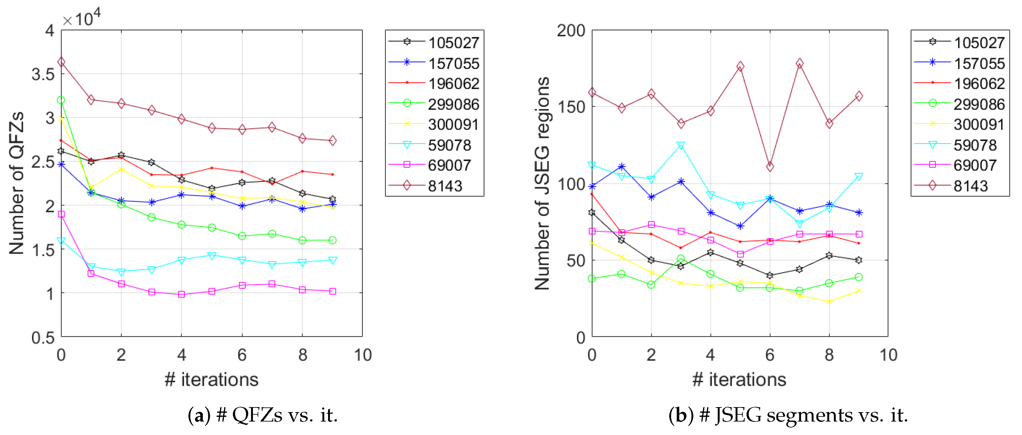
3. Experimental Results
4. Conclusions
Author Contributions
Funding
Conflicts of Interest
References
- Ivanovici, M.; Richard, N.; Paulus, D. Color Image Segmentation. In Advanced Color Image Processing and Analysis; Fernandez-Maloigne, C., Ed.; Springer: New York, NY, USA, 2013; Chapter 8; pp. 219–277. [Google Scholar]
- Mori, G.; Ren, X.; Efros, A.A.; Malik, J. Recovering human body configurations: Combining segmentation and recognition. In Proceedings of the 2004 IEEE Computer Society Conference on Computer Vision and Pattern Recognition, CVPR 2004, Washington, DC, USA, 27 June–2 July 2004; Volume 2, p. II. [Google Scholar]
- Levinshtein, A.; Stere, A.; Kutulakos, K.N.; Fleet, D.J.; Dickinson, S.J.; Siddiqi, K. TurboPixels: Fast Superpixels Using Geometric Flows. IEEE Trans. Pattern Anal. Mach. Intell. 2009, 31, 2290–2297. [Google Scholar] [CrossRef] [Green Version]
- Yang, D.; Huang, J.; Zhang, J.; Zhang, R. Cascaded superpixel pedestrian object segmentation algorithm. In Proceedings of the 2018 Chinese Control and Decision Conference (CCDC), Liaoning, China, 9–11 June 2018; pp. 5975–5978. [Google Scholar]
- Costa, A.L. Developing Minds: A Resource Book for Teaching Thinking, 3rd ed.; Association for Supervision and Curriculum Development: Alexandria, VA, USA, 2001. [Google Scholar]
- Dodge, J. Differentiation in Action; Scholastic Teaching Resources: New York, NY, USA, 2005. [Google Scholar]
- Sousa, D.A. How the Brain Learns: A Classroom Teacher’s Guide; Corwin Press: Thousand Oaks, CA, USA, 2001. [Google Scholar]
- Hattie, J.; Fisher, D.; Frey, N.; Gojak, L.M.; Moore, S.D.; Mellman, W. Visible Learning for Mathematics, Grades K-12: What Works Best to Optimize Student Learning; Corwin Press: Thousand Oaks, CA, USA, 2016. [Google Scholar]
- Knuth, D.E. The Art of Computer Programming: Fundamental Algorithms, 3rd ed.; Addison Wesley Longman Publishing Co., Inc.: Boston, MA, USA, 1997; Volume 1. [Google Scholar]
- Marfil, R.; Molina-Tanco, L.; Bandera, A.; Rodríguez, J.; Sandoval, F. Pyramid segmentation algorithms revisited. Pattern Recognit. 2006, 39, 1430–1451. [Google Scholar] [CrossRef] [Green Version]
- Kass, M.; Witkin, A.; Terzopoulos, D. Snakes: Active contour models. Int. J. Comput. Vis. 1988, 1, 321–331. [Google Scholar] [CrossRef]
- Liu, D.; Xiong, Y.; Pulli, K.; Shapiro, L. Estimating image segmentation difficulty. In International Workshop on Machine Learning and Data Mining in Pattern Recognition; Springer: Berlin/Heidelberg, Germany, 2011; pp. 484–495. [Google Scholar]
- Birkhoff, G.D. Aesthetic Measure; Harvard University: Cambridge, MA, USA, 1933. [Google Scholar]
- Berlyne, D.E. The influence of complexity and novelty in visual figures on orienting responses. J. Exp. Psychol. 1958, 55, 289–296. [Google Scholar] [CrossRef] [PubMed]
- Leeuwenberg, E.L.J. A Perceptual Coding Language for Visual and Auditory Patterns. Am. J. Psychol. 1971, 84, 307–349. [Google Scholar] [CrossRef] [PubMed]
- García, M.; Badre, A.N.; Stasko, J.T. Development and validation of icons varying in their abstractness. Interact. Comput. 1994, 6, 191–211. [Google Scholar] [CrossRef]
- McDougall, S.J.; Curry, M.B.; de Bruijn, O. Measuring symbol and icon characteristics: Norms for concreteness, complexity, meaningfulness, familiarity, and semantic distance for 239 symbols. Behav. Res. Methods Instrum. Comput. 1999, 31, 487–519. [Google Scholar] [CrossRef] [Green Version]
- Olivia, A.; Mack, M.L.; Shrestha, M.; Peeper, A.S. Identifying the Perceptual Dimensions of Visual Complexity of Scenes. In Proceedings of the 26th Annual Meeting of the Cognitive Science Society, Chicago, IL, USA, 4–7 August 2004. [Google Scholar]
- Perkiö, J.; Hyvärinen, A. Modelling Image Complexity by Independent Component Analysis, with Application to Content-Based Image Retrieval. In Artificial Neural Networks—ICANN 2009; Alippi, C., Polycarpou, M., Panayiotou, C., Ellinas, G., Eds.; Springer: Berlin/Heidelberg, Germany, 2009; pp. 704–714. [Google Scholar]
- Da Silva, M.P.; Courboulay, V.; Estraillier, P. Image complexity measure based on visual attention. In Proceedings of the 2011 18th IEEE International Conference on Image Processing, Brussels, Belgium, 11–14 September 2011; pp. 3281–3284. [Google Scholar]
- Forsythe, A.; Nadal, M.; Sheehy, N.; Cela-Conde, C.J.; Sawey, M. Predicting beauty: Fractal dimension and visual complexity in art. Br. J. Psychol. 2011, 102, 49–70. [Google Scholar] [CrossRef] [Green Version]
- Yu, H.; Winkler, S. Image complexity and spatial information. In Proceedings of the 2013 Fifth International Workshop on Quality of Multimedia Experience (QoMEX), Klagenfurt am Wörthersee, Austria, 3–5 July 2013; pp. 12–17. [Google Scholar]
- Corchs, S.E.; Ciocca, G.; Bricolo, E.; Gasparini, F. Predicting Complexity Perception of Real World Images. PLoS ONE 2016, 11, 1–22. [Google Scholar] [CrossRef] [Green Version]
- Guo, X.; Qian, Y.; Li, L.; Asano, A. Assessment model for perceived visual complexity of painting images. Knowl.-Based Syst. 2018, 159, 110–119. [Google Scholar] [CrossRef]
- Serra, J.; Salembier, P. Connected operators and pyramids. In SPIE’s 1993 International Symposium on Optics, Imaging, and Instrumentation; International Society for Optics and Photonics: San Diego, CA, USA, 1993; pp. 65–76. [Google Scholar]
- Soille, P. Constrained connectivity for hierarchical image partitioning and simplification. IEEE Trans. Pattern Anal. Mach. Intell. 2008, 30, 1132–1145. [Google Scholar] [CrossRef] [PubMed]
- Deng, Y.; Manjunath, B.S.; Shin, H. Color image segmentation. In Proceedings of the IEEE Computer Society Conference on Computer Vision and Pattern Recognition CVPR’99, San Francisco, CA, USA, 18–20 June 1996; Volume 2, pp. 446–451. [Google Scholar]
- Deng, Y.; Manjunath, B.S. Unsupervised segmentation of color-texture regions in images and video. IEEE Trans. Pattern Anal. Mach. Intell. 2001, 23, 800–810. [Google Scholar] [CrossRef] [Green Version]
- Ivanovici, M.; Richard, N. Fractal Dimension of Colour Fractal Images. IEEE Trans. Image Process. 2011, 20, 227–235. [Google Scholar] [CrossRef] [PubMed]
- Ivanovici, M. Color Fractal Images with Independent RGB Color Components. 2019. Available online: https://ieee-dataport.org/open-access/color-fractal-images-independent-rgb-color-components (accessed on 25 November 2019).
- Arbelaez, P.; Maire, M.; Fowlkes, C.; Malik, J. Contour detection and hierarchical image segmentation. IEEE Trans. Pattern Anal. Mach. Intell. 2011, 33, 898–916. [Google Scholar] [CrossRef] [PubMed] [Green Version]
- Shannon, C. A mathematical theory of communication. Bell Syst. Tech. J. 1948, 27, 379–423. [Google Scholar] [CrossRef] [Green Version]
- Pham, T.D. The Kolmogorov-Sinai Entropy in the Setting of Fuzzy Sets for Image Texture Analysis and Classification. Pattern Recognit. 2016, 53, 229–237. [Google Scholar] [CrossRef]
- Haralick, R.M.; Shanmugam, K.; Dinstein, I. Textural Features for Image Classification. IEEE Trans. Syst. Man Cybern. 1973, SMC-3, 610–621. [Google Scholar] [CrossRef] [Green Version]
- Ivanovici, M.; Richard, N. Entropy versus fractal complexity for computer-generated color fractal images. In Proceedings of the 4th CIE Expert Symposium on Colour and Visual Appearance, Prague, Czech Republic, 6–7 September 2016. [Google Scholar]
- Mandelbrot, B. The Fractal Geometry of Nature; W.H. Freeman and Co.: New York, NY, USA, 1982. [Google Scholar]
- Peitgen, H.; Saupe, D. The Sciences of Fractal Images; Springer: Berlin/Heidelberg, Germany, 1988. [Google Scholar]
- Chen, W.; Yuan, S.; Hsiao, H.; Hsieh, C. Algorithms to estimating fractal dimension of textured images. In Proceedings of the 2001 IEEE International Conference on Acoustics, Speech, and Signal Processing, Salt Lake City, UT, USA, 7–11 May 2001; Volume 3, pp. 1541–1544. [Google Scholar]
- Falconer, K. Fractal Geometry, Mathematical Foundations and Applications; John Wiley and Sons: Hoboken, NJ, USA, 1990. [Google Scholar]
- Voss, R. Random Fractals: Characterization and measurement. Scaling Phenom. Disord. Syst. 1986, 10, 51–61. [Google Scholar] [CrossRef]
- Keller, J.; Chen, S. Texture Description and segmentation through Fractal Geometry. Comput. Vis. Graph. Image Process. 1989, 45, 150–166. [Google Scholar] [CrossRef]
- Maragos, P.; Sun, F. Measuring the fractal dimension of signals: Morphological covers and iterative optimization. IEEE Trans. Signal Process. 1993, 41, 108–121. [Google Scholar] [CrossRef]
- Allain, C.; Cloitre, M. Characterizing the lacunarity of random and deterministic fractal sets. Phys. Rev. A 1991, 44, 3552–3558. [Google Scholar] [CrossRef] [PubMed]
- Manousaki, A.G.; Manios, A.G.; Tsompanaki, E.I.; Tosca, A.D. Use of color texture in determining the nature of melanocytic skin lesions—A qualitative and quantitative approach. Comput. Biol. Med. 2006, 36, 416–427. [Google Scholar] [CrossRef] [PubMed]
- Zhao, X.; Wang, X. Fractal Dimension Estimation of RGB Color Images Using Maximum Color Distance. Fractals 2016, 24. [Google Scholar] [CrossRef]
- Nayak, S.R.; Mishra, J. An improved method to estimate the fractal dimension of colour images. Perspect. Sci. 2016, 8, 412–416. [Google Scholar] [CrossRef] [Green Version]
- Nayak, S.R.; Mishra, J.; Khandual, A.; Palai, G. Fractal dimension of RGB color images. Optik 2018, 162, 196–205. [Google Scholar] [CrossRef]
- Coliban, R.M.; Ivanovici, M. Reducing the oversegmentation induced by quasi-flat zones for multivariate images. J. Vis. Commun. Image Represent. 2018, 53, 281–293. [Google Scholar] [CrossRef]
- Rigau, J.; Feixas, M.; Sbert, M. An Information-Theoretic Framework for Image Complexity. In Computational Aesthetics’05: Proceedings of the First Eurographics Conference on Computational Aesthetics in Graphics, Visualization and Imaging; Eurographics Association: Goslar, Germany, 2005; pp. 177–184. [Google Scholar]


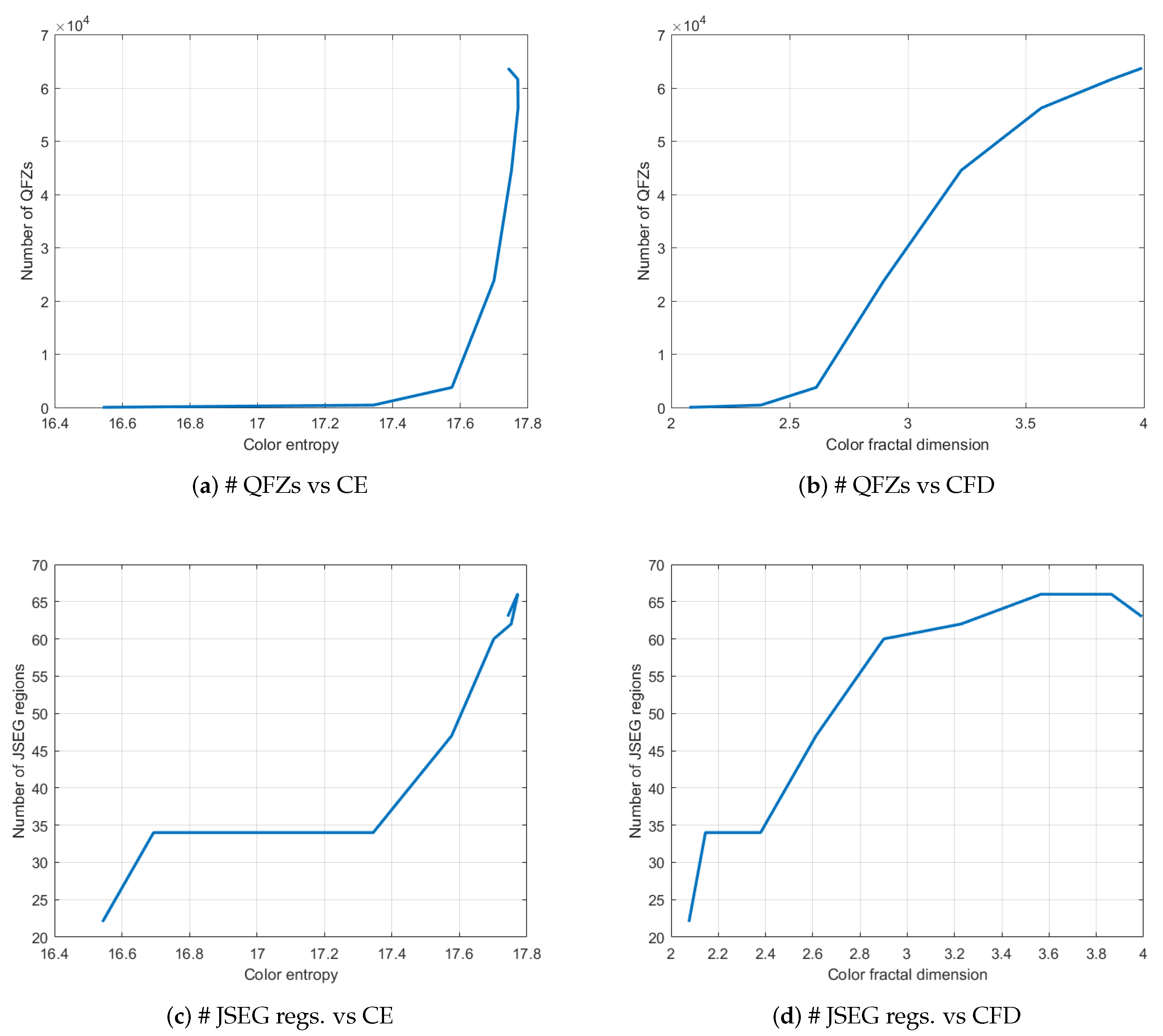
| H = 0.1 | H = 0.2 | H = 0.3 | H = 0.4 | H = 0.5 | H = 0.6 | H = 0.7 | H = 0.8 | H = 0.9 | |
|---|---|---|---|---|---|---|---|---|---|
| CE | 17.7429 | 17.772 | 17.7727 | 17.7532 | 17.7015 | 17.5768 | 17.3444 | 16.6938 | 16.5423 |
| CFD | 3.9926 | 3.8637 | 3.5655 | 3.2269 | 2.9002 | 2.6137 | 2.3791 | 2.1456 | 2.0757 |
| # QFZs | 63694 | 61597 | 56191 | 44503 | 23829 | 3755 | 437 | 101 | 20 |
| # JSEG regs. | 63 | 66 | 66 | 62 | 60 | 47 | 34 | 34 | 22 |
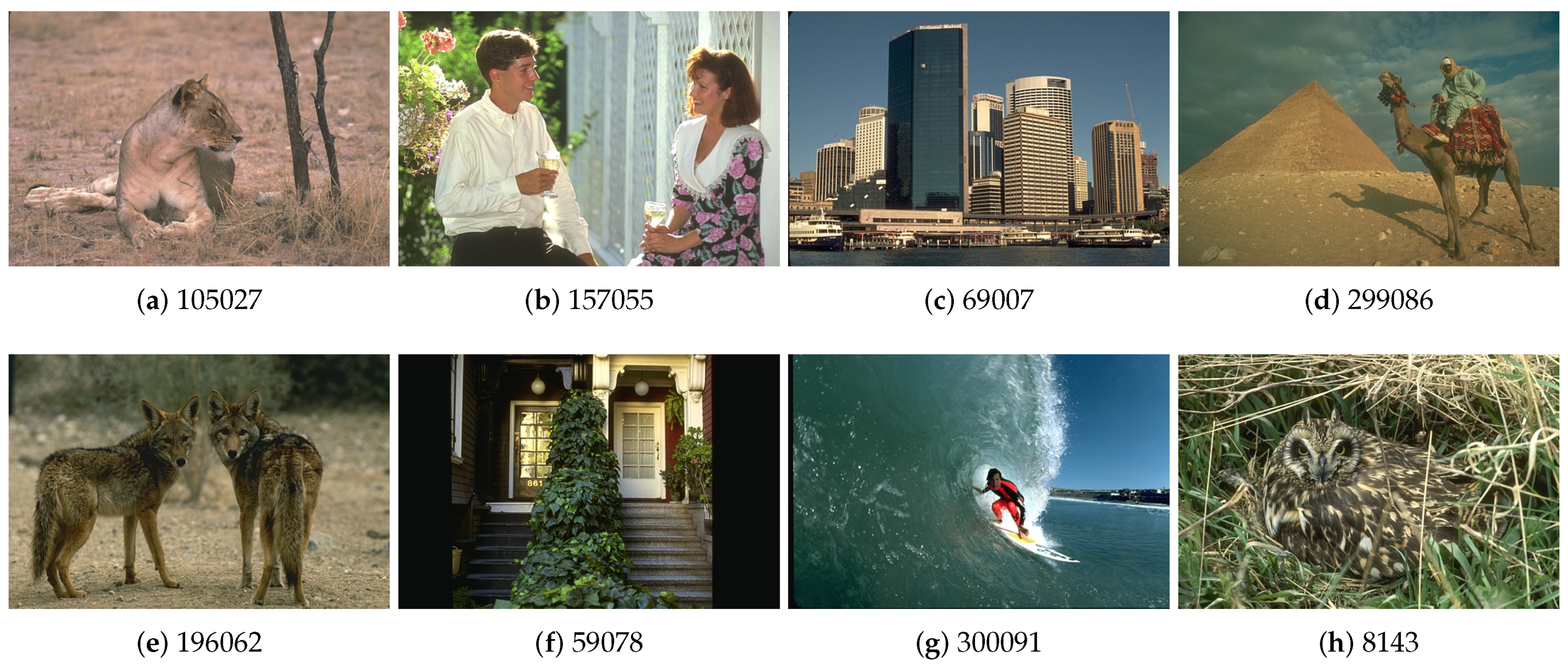
| Image | 105027 | 157055 | 69007 | 299086 | 196062 | 59078 | 300091 | 8143 |
|---|---|---|---|---|---|---|---|---|
| CE | 12.7748 | 14.4893 | 13.0638 | 12.9328 | 13.0152 | 11.0511 | 12.6644 | 15.3425 |
| CFD | 2.9631 | 3.1163 | 3.1132 | 2.9468 | 2.9502 | 3.1163 | 2.7797 | 3.2685 |
| # QFZs | 26164 | 24641 | 27389 | 31982 | 29882 | 16025 | 18951 | 36335 |
| # JSEG regs. | 81 | 98 | 93 | 38 | 61 | 112 | 69 | 159 |
© 2020 by the authors. Licensee MDPI, Basel, Switzerland. This article is an open access article distributed under the terms and conditions of the Creative Commons Attribution (CC BY) license (http://creativecommons.org/licenses/by/4.0/).
Share and Cite
Ivanovici, M.; Coliban, R.-M.; Hatfaludi, C.; Nicolae, I.E. Color Image Complexity versus Over-Segmentation: A Preliminary Study on the Correlation between Complexity Measures and Number of Segments. J. Imaging 2020, 6, 16. https://0-doi-org.brum.beds.ac.uk/10.3390/jimaging6040016
Ivanovici M, Coliban R-M, Hatfaludi C, Nicolae IE. Color Image Complexity versus Over-Segmentation: A Preliminary Study on the Correlation between Complexity Measures and Number of Segments. Journal of Imaging. 2020; 6(4):16. https://0-doi-org.brum.beds.ac.uk/10.3390/jimaging6040016
Chicago/Turabian StyleIvanovici, Mihai, Radu-Mihai Coliban, Cosmin Hatfaludi, and Irina Emilia Nicolae. 2020. "Color Image Complexity versus Over-Segmentation: A Preliminary Study on the Correlation between Complexity Measures and Number of Segments" Journal of Imaging 6, no. 4: 16. https://0-doi-org.brum.beds.ac.uk/10.3390/jimaging6040016