Evaluation of the Weighted Mean X-ray Energy for an Imaging System Via Propagation-Based Phase-Contrast Imaging

 , , , , , , , and
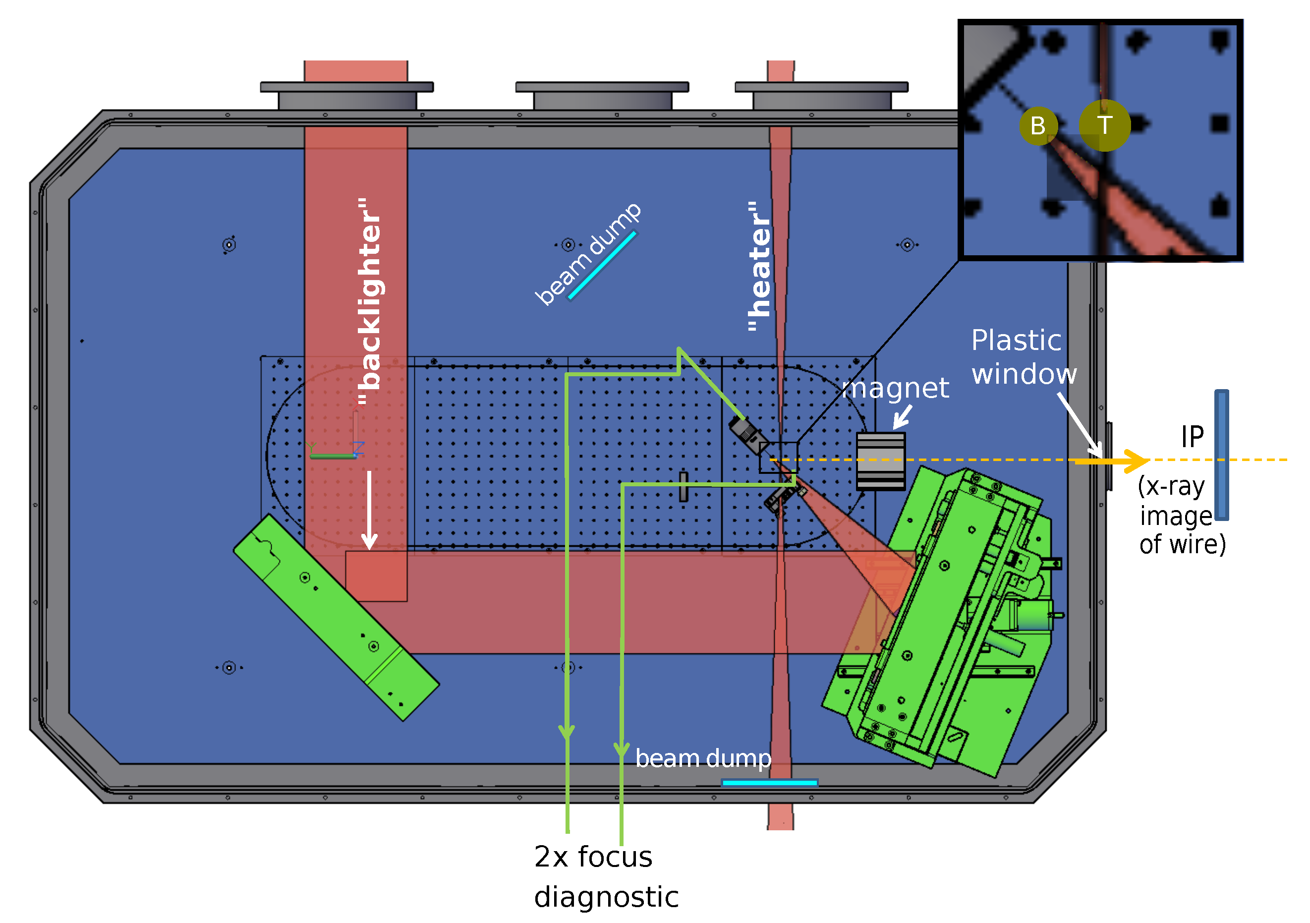
Abstract
:1. Introduction
2. Materials and Methods
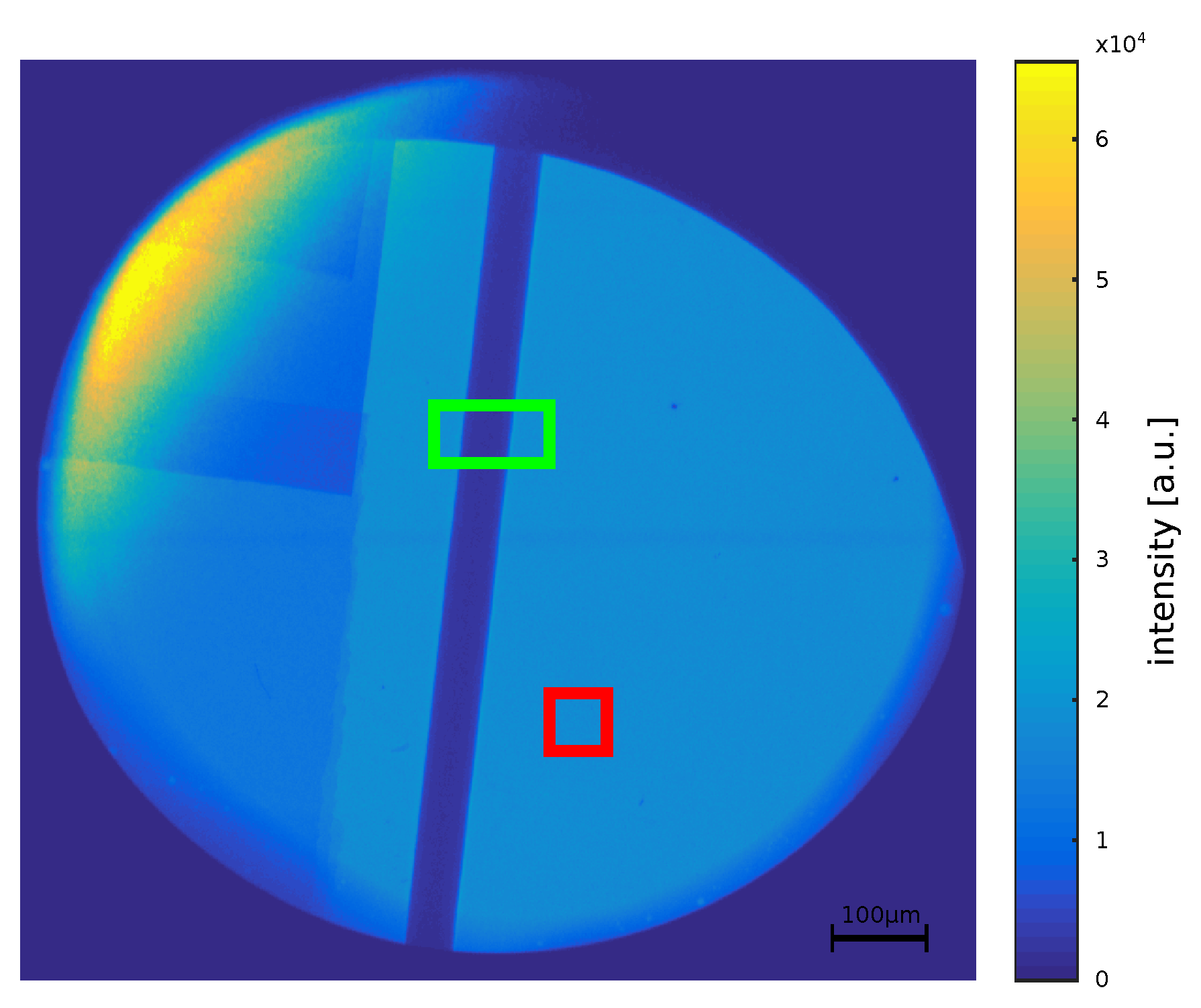
2.1. Measurement Setup at GSI
2.2. Measurement Setup at DLS
2.3. Propagation-Based Phase-Contrast
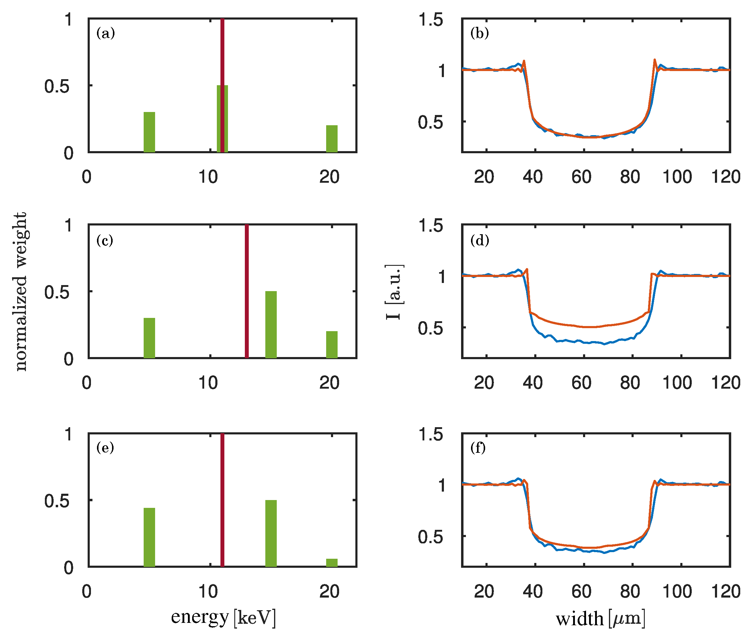
2.4. Computer Simulation
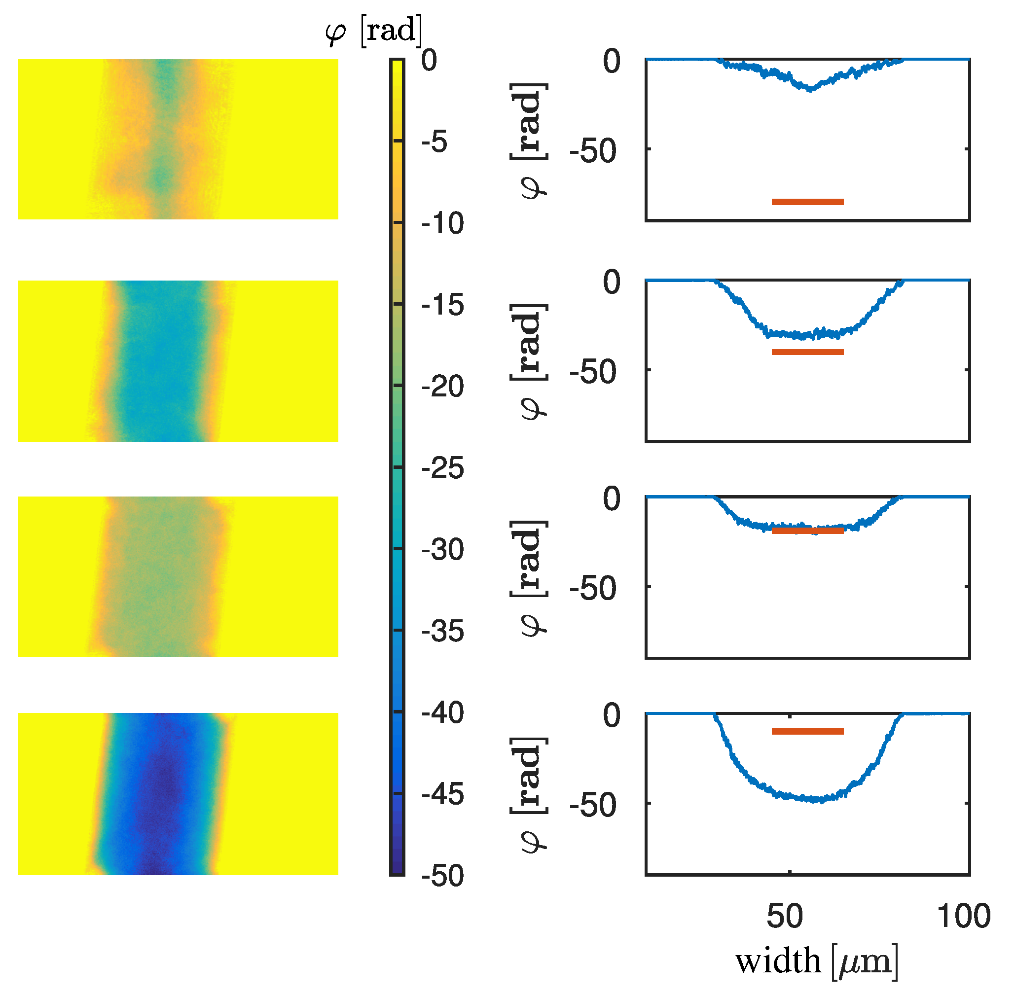
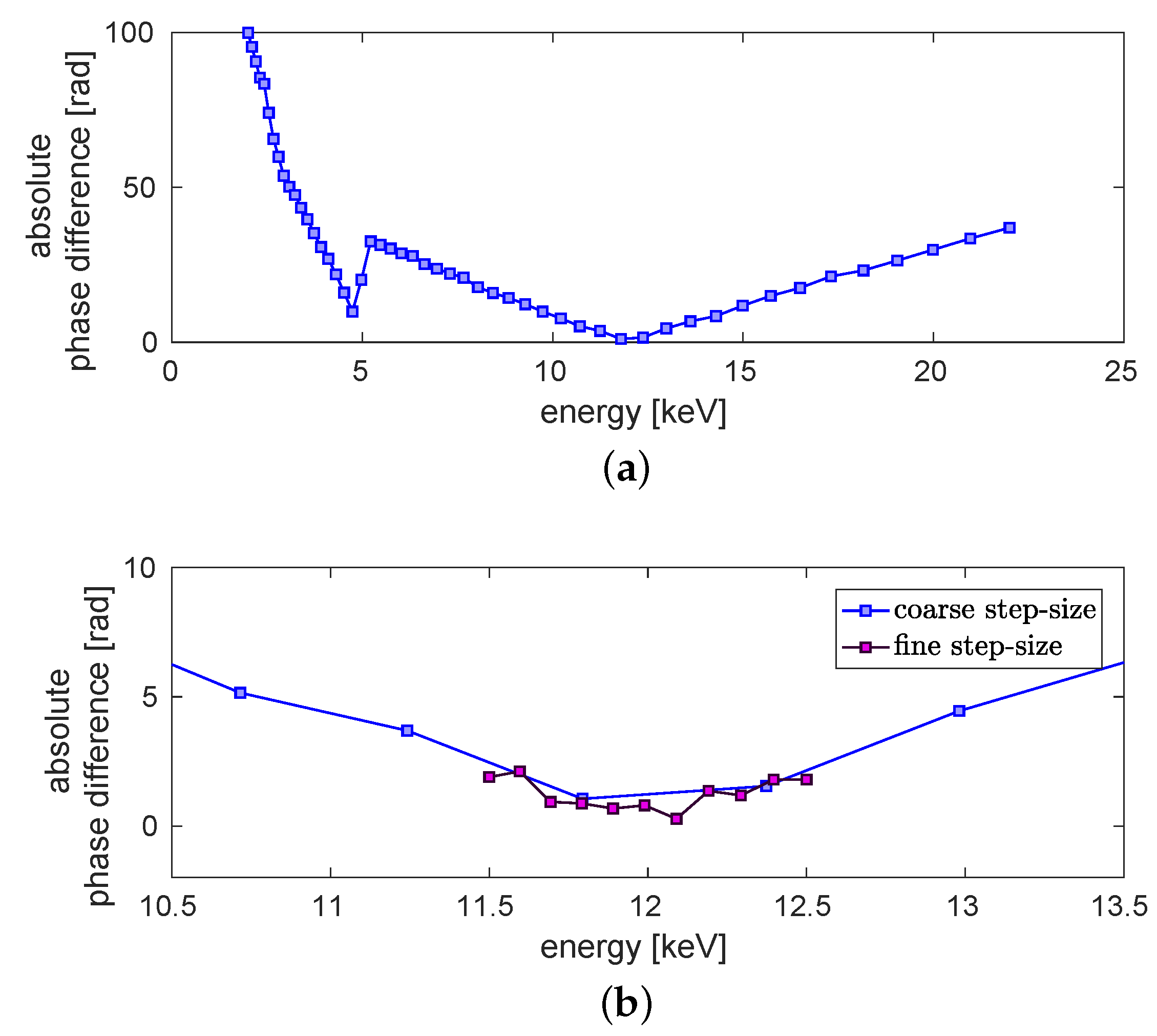
2.5. Energy Evaluation for GSI Data
3. Results
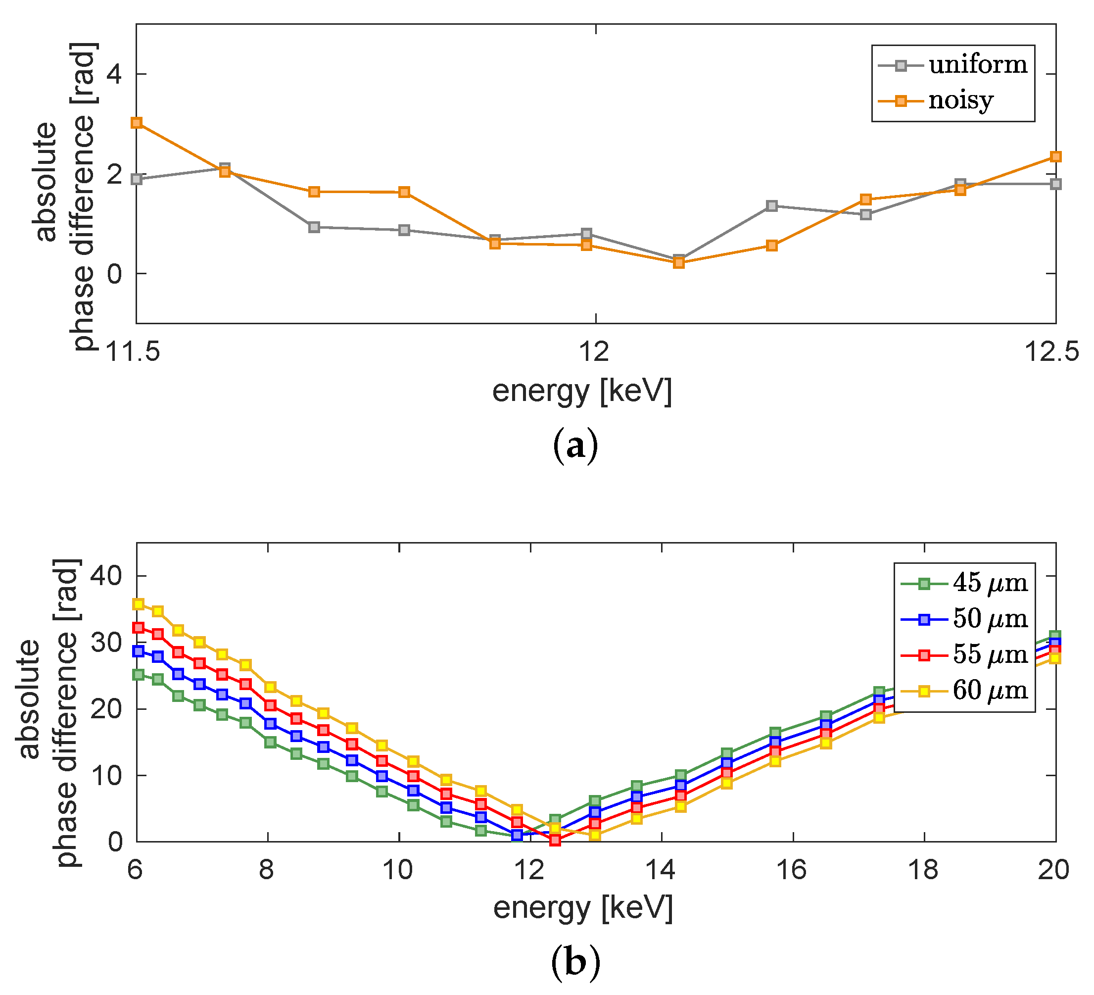
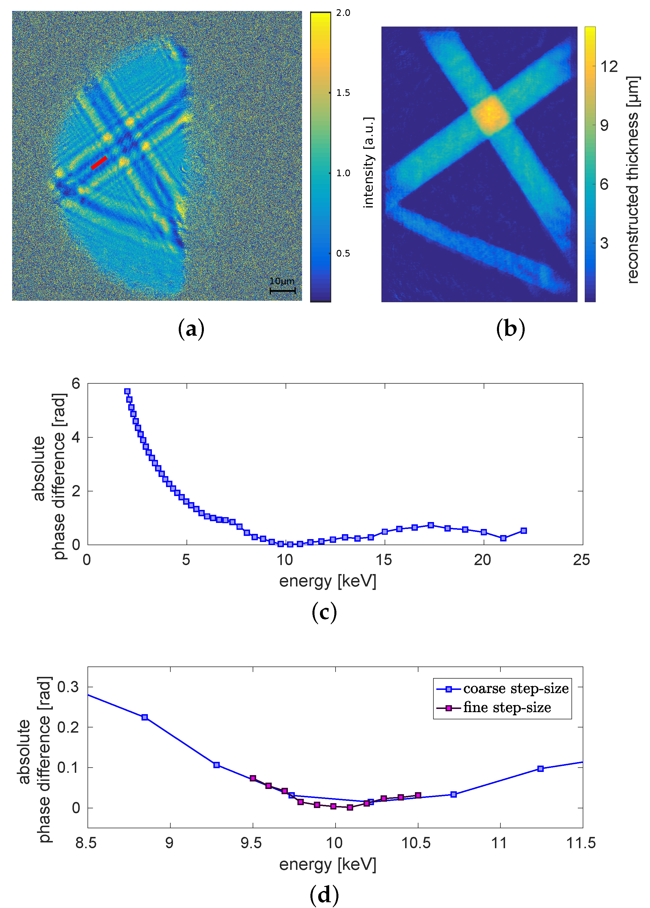
3.1. Evaluation of the Dominant X-ray Energy
3.2. Validation of the Evaluated Dominant X-ray Energy
3.3. Validation of the Evaluation Method with Monochromatic Images
4. Discussion and Conclusions
Author Contributions
Funding
Acknowledgments
Conflicts of Interest
References
- Le Pape, S.; Neumayer, P.; Fortmann, C.; Döppner, T.; Davis, P.; Kritcher, A.; Landen, O.; Glenzer, S. X-ray radiography and scattering diagnosis of dense shock-compressed matter. Phys. Plasmas 2010, 17, 056309. [Google Scholar] [CrossRef] [Green Version]
- Hochhaus, D.C.; Aurand, B.; Basko, M.; Ecker, B.; Kühl, T.; Ma, T.; Rosmej, F.; Zielbauer, B.; Neumayer, P. X-ray radiographic expansion measurements of isochorically heated thin wire targets. Phys. Plasmas 2013, 20, 062703. [Google Scholar] [CrossRef] [Green Version]
- Schwoerer, H.; Gibbon, P.; Düsterer, S.; Behrens, R.; Ziener, C.; Reich, C.; Sauerbrey, R. MeV X Rays and Photoneutrons from Femtosecond Laser-Produced Plasmas. Phys. Rev. Lett. 2001, 86, 2317–2320. [Google Scholar] [CrossRef] [PubMed] [Green Version]
- Momose, A. Demonstration of phase-contrast X-ray computed tomography using an X-ray interferometer. Nucl. Instrum. Methods Phys. Res. Sect. Accel. Spectrom. Detect. Assoc. Equip. 1995, 352, 622–628. [Google Scholar] [CrossRef]
- Momose, A. Recent Advances in X-ray Phase Imaging. Jpn. J. Appl. Phys. 2005, 44, 6355. [Google Scholar] [CrossRef]
- Pfeiffer, F.; Weitkamp, T.; Bunk, O.; David, C. Phase retrieval and differential phase-contrast imaging with low-brilliance X-ray sources. Nat. Phys. 2006, 2, 258–261. [Google Scholar] [CrossRef]
- Willner, M.; Herzen, J.; Grandl, S.; Auweter, S.; Mayr, D.; Hipp, A.; Chabior, M.; Sarapata, A.; Achterhold, K.; Zanette, I.; et al. Quantitative breast tissue characterization using grating-based X-ray phase-contrast imaging. Phys. Med. Biol. 2014, 59, 1557–1571. [Google Scholar] [CrossRef]
- Myers, G.R.; Mayo, S.C.; Gureyev, T.E.; Paganin, D.M.; Wilkins, S.W. Polychromatic cone-beam phase-contrast tomography. Phys. Rev. A 2007, 76, 045804. [Google Scholar] [CrossRef]
- Wilkins, S.; Gureyev, T.E.; Gao, D.; Pogany, A.; Stevenson, A. Phase-contrast imaging using polychromatic hard X-rays. Nature 1996, 384, 335. [Google Scholar] [CrossRef]
- Snigirev, A.; Snigireva, I.; Kohn, V.; Kuznetsov, S.; Schelokov, I. On the possibilities of X-ray phase contrast microimaging by coherent high-energy synchrotron radiation. Rev. Sci. Instrum. 1995, 66, 5486–5492. [Google Scholar] [CrossRef]
- Meadowcroft, A.L.; Bentley, C.D.; Stott, E.N. Evaluation of the sensitivity and fading characteristics of an image plate system for X-ray diagnostics. Rev. Sci. Instrum. 2008, 79, 113102. [Google Scholar] [CrossRef]
- Clark, J.N.; Putkunz, C.T.; Pfeifer, M.A.; Peele, A.G.; Williams, G.J.; Chen, B.; Nugent, K.A.; Hall, C.; Fullagar, W.; Kim, S.; et al. Use of a complex constraint in coherent diffractive imaging. Opt. Express 2010, 18, 1981. [Google Scholar] [CrossRef] [PubMed]
- Bagnoud, V.; Aurand, B.; Blazevic, A.; Borneis, S.; Bruske, C.; Ecker, B.; Eisenbarth, U.; Fils, J.; Frank, A.; Gaul, E.; et al. Commissioning and early experiments of the PHELIX facility. Appl. Phys. B 2010, 100, 137–150. [Google Scholar] [CrossRef]
- Antonelli, L.; Barbato, F.; Mancelli, D.; Trela, J.; Zeraouli, G.; Boutoux, G.; Neumayer, P.; Atzeni, S.; Schiavi, A.; Volpe, L.; et al. X-ray phase-contrast imaging for laser-induced shock waves. EPL (Europhys. Lett.) 2019, 125, 35002. [Google Scholar] [CrossRef] [Green Version]
- Schropp, A.; Hoppe, R.; Meier, V.; Patommel, J.; Seiboth, F.; Ping, Y.; Hicks, D.G.; Beckwith, M.A.; Collins, G.W.; Higginbotham, A.; et al. Imaging Shock Waves in Diamond with Both High Temporal and Spatial Resolution at an XFEL. Sci. Rep. 2015, 5. [Google Scholar] [CrossRef] [Green Version]
- Fiksel, G.; Marshall, F.J.; Mileham, C.; Stoeckl, C. Note: Spatial resolution of Fuji BAS-TR and BAS-SR imaging plates. Rev. Sci. Instrum. 2012, 83, 086103. [Google Scholar] [CrossRef]
- Weitkamp, T.; Haas, D.; Wegrzynek, D.; Rack, A. ANKAphase: Software for single-distance phase retrieval from inline X-ray phase-contrast radiographs. J. Synchrotron Radiat. 2011, 18, 617–629. [Google Scholar] [CrossRef] [PubMed]
- Burvall, A.; Lundström, U.; Takman, P.A.C.; Larsson, D.H.; Hertz, H.M. Phase retrieval in X-ray phase-contrast imaging suitable for tomography. Opt. Express 2011, 19, 10359–10376. [Google Scholar] [CrossRef] [PubMed]
- Souvorov, A.; Ishikawa, T.; Kuyumchyan, A. Multiresolution phase retrieval in the Fresnel region by use of wavelet transform. J. Opt. Soc. Am. Opt. Image Sci. 2006, 23, 279–287. [Google Scholar] [CrossRef]
- Voelz, D.G. Computational Fourier Optics: A MATLAB Tutorial; SPIE Press: Bellingham, WA, USA, 2011. [Google Scholar]
- Giewekemeyer, K.; Krüger, S.P.; Kalbfleisch, S.; Bartels, M.; Beta, C.; Salditt, T. X-ray propagation microscopy of biological cells using waveguides as a quasipoint source. Phys. Rev. A 2011, 83. [Google Scholar] [CrossRef]
- Hagemann, J.; Salditt, T. Divide and update: Towards single-shot object and probe retrieval for near-field holography. Opt. Express 2017, 25, 20953–20968. [Google Scholar] [CrossRef] [PubMed] [Green Version]
- Paganin, D.M. Coherent X-ray Optics; Oxford University Press (OUP): Oxford, UK, 2006. [Google Scholar] [CrossRef]
- Paganin, D.; Mayo, S.C.; Gureyev, T.E.; Miller, P.R.; Wilkins, S.W. Simultaneous phase and amplitude extraction from a single defocused image of a homogeneous object. J. Microsc. 2002, 206, 33–40. [Google Scholar] [CrossRef] [PubMed]
- Bronnikov, A.V. Reconstruction formulas in phase-contrast tomography. Opt. Commun. 1999, 171, 239–244. [Google Scholar] [CrossRef]
- Cloetens, P.; Ludwig, W.; Baruchel, J.; Van Dyck, D.; Van Landuyt, J.; Guigay, J.P.; Schlenker, M. Holotomography: Quantitative phase tomography with micrometer resolution using hard synchrotron radiation X-rays. Appl. Phys. Lett. 1999, 75, 2912–2914. [Google Scholar] [CrossRef] [Green Version]
- Guigay, J.P.; Langer, M.; Boistel, R.; Cloetens, P. Mixed transfer function and transport of intensity approach for phase retrieval in the Fresnel region. Opt. Lett. 2007, 32, 1617–1619. [Google Scholar] [CrossRef]
- Henke, B.; Gullikson, E.; Davis, J. X-ray interactions: Photoabsorption, scattering, transmission, and reflection at E = 50–30,000 eV, Z = 1–92. At. Data Nucl. Data Tables 1993, 54, 181–342. [Google Scholar] [CrossRef] [Green Version]
- Morgan, K.S.; Siu, K.K.W.; Paganin, D.M. The projection approximation and edge contrast for X-ray propagation-based phase contrast imaging of a cylindrical edge. Opt. Express 2010, 18, 9865–9878. [Google Scholar] [CrossRef]
- Matsushima, K.; Shimobaba, T. Band-Limited Angular Spectrum Method for Numerical Simulation of Free-Space Propagation in Far and Near Fields. Opt. Express 2009, 17, 19662–19673. [Google Scholar] [CrossRef] [Green Version]
- Bearden, J.A. X-ray Wavelengths. Rev. Mod. Phys. 1967, 39, 78–124. [Google Scholar] [CrossRef]


© 2020 by the authors. Licensee MDPI, Basel, Switzerland. This article is an open access article distributed under the terms and conditions of the Creative Commons Attribution (CC BY) license (http://creativecommons.org/licenses/by/4.0/).
Share and Cite
Seifert, M.; Weule, M.; Cipiccia, S.; Flenner, S.; Hagemann, J.; Ludwig, V.; Michel, T.; Neumayer, P.; Schuster, M.; Wolf, A.; et al. Evaluation of the Weighted Mean X-ray Energy for an Imaging System Via Propagation-Based Phase-Contrast Imaging. J. Imaging 2020, 6, 63. https://0-doi-org.brum.beds.ac.uk/10.3390/jimaging6070063
Seifert M, Weule M, Cipiccia S, Flenner S, Hagemann J, Ludwig V, Michel T, Neumayer P, Schuster M, Wolf A, et al. Evaluation of the Weighted Mean X-ray Energy for an Imaging System Via Propagation-Based Phase-Contrast Imaging. Journal of Imaging. 2020; 6(7):63. https://0-doi-org.brum.beds.ac.uk/10.3390/jimaging6070063
Chicago/Turabian StyleSeifert, Maria, Mareike Weule, Silvia Cipiccia, Silja Flenner, Johannes Hagemann, Veronika Ludwig, Thilo Michel, Paul Neumayer, Max Schuster, Andreas Wolf, and et al. 2020. "Evaluation of the Weighted Mean X-ray Energy for an Imaging System Via Propagation-Based Phase-Contrast Imaging" Journal of Imaging 6, no. 7: 63. https://0-doi-org.brum.beds.ac.uk/10.3390/jimaging6070063