Identification of QR Code Perspective Distortion Based on Edge Directions and Edge Projections Analysis


1
Technical University in Zvolen, Faculty of Technology, Department of Manufacturing and Automation Technology, Masarykova 24, 960 01 Zvolen, Slovakia
2
Slovak University of Technology in Bratislava, Faculty of Materials Science and Technology in Trnava, Institute of Production Technologies, 917 24 Trnava, Slovakia
*
Author to whom correspondence should be addressed.
J. Imaging 2020, 6(7), 67; https://0-doi-org.brum.beds.ac.uk/10.3390/jimaging6070067
Submission received: 22 June 2020
/
Revised: 6 July 2020
/
Accepted: 8 July 2020
/
Published: 10 July 2020
Abstract
:QR (quick response) Codes are one of the most popular types of two-dimensional (2D) matrix codes currently used in a wide variety of fields. Two-dimensional matrix codes, compared to 1D bar codes, can encode significantly more data in the same area. We have compared algorithms capable of localizing multiple QR Codes in an image using typical finder patterns, which are present in three corners of a QR Code. Finally, we present a novel approach to identify perspective distortion by analyzing the direction of horizontal and vertical edges and by maximizing the standard deviation of horizontal and vertical projections of these edges. This algorithm is computationally efficient, works well for low-resolution images, and is also suited to real-time processing.
1. Introduction
Two-dimensional (2D) matrix codes are a way how to efficiently store data that are machine readable. Thanks to the great spread of smartphones, 2D matrix codes have found application in many areas of life and industry. QR (quick response) Code was invented in 1994 by Denso Wave for the automotive industry in Japan, but nowadays has much wider usage. They are widely used in segments such as manufacturing, logistics, sales, media, advertising, tourism, e-commerce, identification, and authentication [1,2]. The QR Code often contains additional information about the product, the object or the place where it is located. However, they can also be a URL to a web page, Global Positioning System (GPS) coordinates, contact details, delivery address, payment instructions, etc.
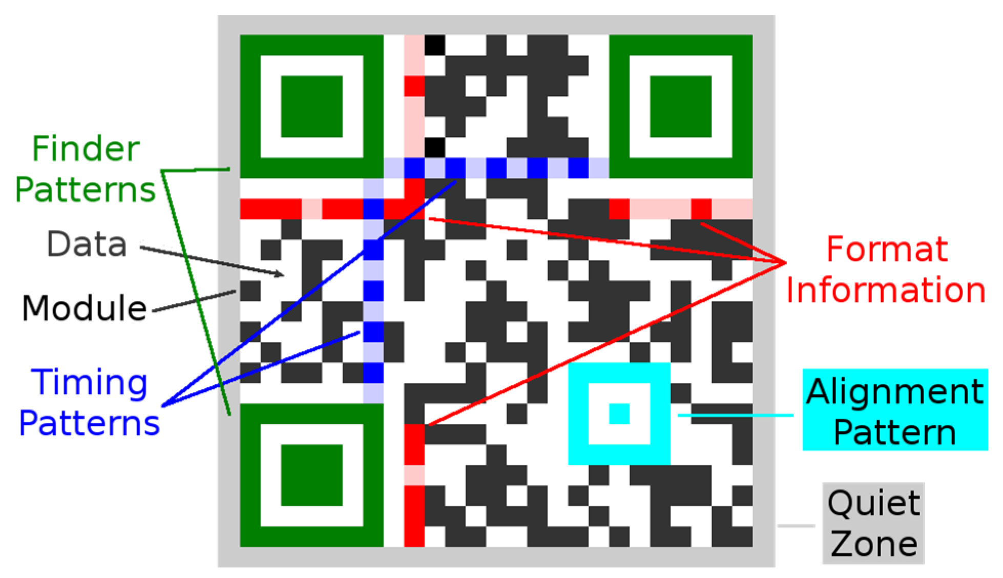
QR codes belong to a group of 2D matrix codes (similarly the data matrix codes). Traditional QR code (QR code Model 1 and Model 2) has a square shape and on its three corners are typical square-shaped patterns—finder patterns (FP), which are used to locate the code and to determine its dimensions and rotation. QR Code is structured as follows (Figure 1).
- Module—the smallest building element of a QR Code represented by a small dark or light square. One module represents one bit: usually, dark module for the “1” and light module for the “0”. Modules are organized into rows and columns and form squared matrix.
- Finder patterns—also called position detection patterns, these are localized in three corners of a QR Code. Each Finder Pattern is formed by an inner dark square (of size 3 × 3 modules) surrounded by a dark frame (of size 7 × 7 modules). Finder Patterns are separated from the rest of a QR Code by a light area of width one module. Finder Patterns are used by readers to determine position and orientation of a QR Code.
- Timing patterns—these are placed inside a QR Code and interconnect finder patterns. Timing patterns are formed by sequence of alternating dark and light modules. The timing pattern is used to determine the size of a module, the number of rows and columns, and possible distortion of a code.
- Alignment patterns—there may be none or more alignment patterns according to a version of a QR Code (QR Code version 1 has no alignment pattern). They allow the scanning device to determine the possible perspective distortion of the QR Code image.
- Format information—this contains additional information such as used error correction level (4 options) or a mask patterns number (7 options), which are required for decoding a QR Code.
- Quiet zone—this is a white area of width at least four modules located around a QR Code (in practice, the width is often less than four modules as required by the standard). The quiet zone should not contain any patterns or structures which can confuse readers.
- Data—they are encoded inside a QR Code and are protected by an error correction carried out via a Reed–Solomon algorithm (allows restoration of damaged data). This also means that a QR Code can be partially damaged and can still be entirely read out. QR Codes provide four user selectable levels of error correction: L (Low), M (Medium), Q (Quartile), and H (High). It means that up to approximately 7%, 15%, 25%, and 30% of the code words, which are damaged, can be restored [3]. Increasing the level of error correction reduces the available data capacity of a QR Code.
QR Codes are available in 40 different versions (version 1 represents a QR Code with 21 × 21 modules and version 40 represents QR Code with 177 × 177 modules; the relation between size and version can be expressed as: Size = 21 + (Version − 1) × 4).
Each QR Code version has the maximum data capacity according to the amount of data, character type and error correction level. For example, there is capacity of 10 alphanumeric (alt. 17 numeric) characters in a QR Code of minimal version 1 (size 21 × 21 modules), and capacity up to 1852 alphanumeric (alt. 3057 numeric) characters in maximal version 40 (size 177 × 177 modules) at highest error correction level [3]. QR Codes are able to encode numeric, alphanumeric, Kanji characters and also binary data.
The rest of this paper is organized as follows: in Section 2 a brief overview of previously published methods is presented, in Section 3 two finder pattern localization methods are summarized, in Section 4 the proposed method for QR Code perspective distortion identification is introduced, and in Section 5 the experimental results are presented.
2. Related Work
There were various approaches for QR Code detection in images published in the past. We can divide them into three main groups.
2.1. Finder Pattern-Based Localization Methods
The first group uses for location of a QR Code features of three typical finder patterns (Figure 1 and Figure 3).
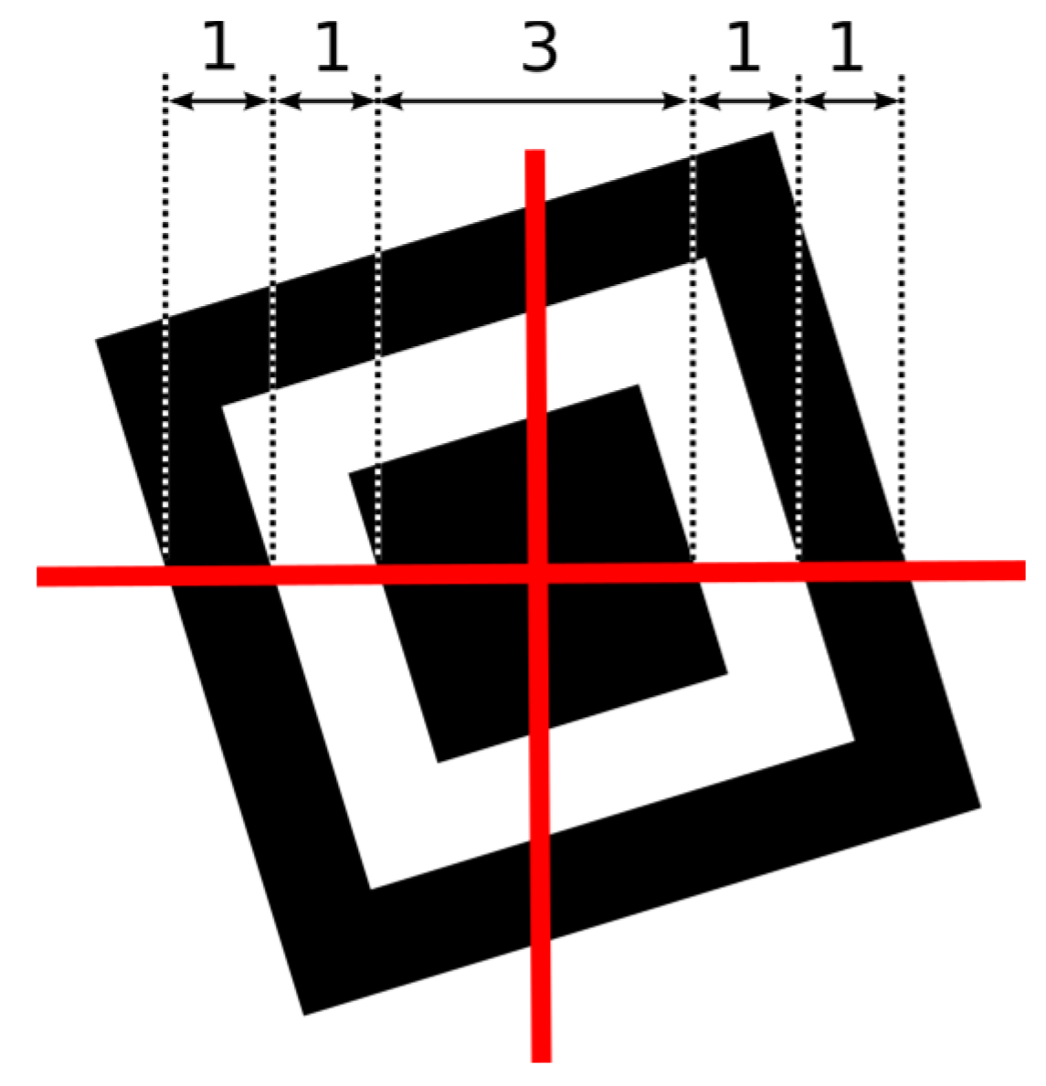
The shape of the finder pattern (square in the frame, Figure 3) was intentionally selected by QR Code inventors because “it was the pattern least likely to appear on various business forms and the like” [4]. They surveyed innumerable examples of printed matter and came up with the least used ratio of black and white areas on printed matter. This ratio was 1:1:3:1:1 (B:W:BBB:W:B), regardless of an angle of scanning.
In Lin and Fuh [5] a binary image is scanned horizontally and then vertically to find all points matching the ratios 1:1:3:1:1. Then the points belonging to the same FP are combined and the angle between three FP is checked.
In Li et al. [6] the connected components in a binary image are compressed using run-length coding on row basis. Then typical ratios of FP are searched row by row. Found FPs establish minimal containing region in which foreground points are searched for ratios 1:3:1, using a modified Knuth–Morris–Pratt algorithm for fast exploration, to compute a centre coordinate of FP.
In Belussi and Hirata [7] they use a cascade of weak classifiers trained on the finder patterns of the QR Code (The Viola-Jones’ rapid object detection method and Haar-like features extracted under floating window are used). In the second stage, the geometrical relationships among detected candidate finder patterns are analyzed in order to verify if there are subgroups of three of them spatially arranged as three corners of a square region.
In Bodnár and Nyúl [8] they also use cascade classifiers using Haar-like features, local binary patterns and histograms of oriented gradients, trained for the finder patterns of QR Codes and for the whole code region as well (also on multiple scales). The training process was too time-consuming.
In Tribak and Zaz [9] the first horizontal and vertical scans are performed to localize preliminarily QR Code patterns, followed by the principal component analysis (PCA) method, which allows removing false positives.
In Tribak and Zaz [10] instead of PCA, the authors use 7 Hu invariant moments as feature descriptors to preliminarily localized FP. The obtained feature vector is compared with feature vectors of set of training samples using Euclidean distance.
2.2. Local Features with Region Growing-Based Localization Methods
The methods in the second group extract specific features from an image under a floating window and these features are checked against sample features. The regions of an image, which are classified as QR Code candidate regions, are merged into larger ones. Local features may be constructed from the Ciążyński and Fabijańska window histogram [11] or from HOG (histogram of oriented gradients), angles of two main gradient directions, a number of edge pixels and an estimation of probability score of a chessboard-like structure Szentandrási et al. [12].
2.3. Connected Components-Based Localization Methods
The third group of methods attempts to detect QR Code as a whole. It is usually based on the fact that a QR Code consists of many small black squares which are relatively close to each other [13,14,15]. Usually, morphological erosion and dilation are applied to connect these small squares into one monolithic object and remove small objects. Gaur and Tiwari [13] proposed to use Canny edge detector together with morphological operations. Kong [14] combined Harris corner detection with convex hull algorithm to get the outline of the outer quadrilateral of a QR Code. In Sun et al. [15] researchers introduce algorithm, which aims to find QR Code area by detection of four corners of 2D barcode. They combine Canny edge detection with contours finding algorithm.
2.4. Deep Learning Based Localization Methods
Hansen et al. [16] described how to adapt deep learning based object detection algorithm YOLO for the purpose of detecting barcodes. Similarly, Zharkov and Zagaynov [17] introduced new fast and robust deep learning detector of 1D and 2D barcodes based on semantic segmentation approach. Convolutional neural network was utilized also in works [18,19].
3. The Finder Pattern Localization Methods
In the following paragraphs, we will give a brief overview of two methods for locating QR Codes which are based on finding three typical patterns—finder patterns—in the corners of the QR Code [5,20]. These three finder patterns also identify the three corner points of the QR Code bounding box. The method for determining the position of the 4th corner of the bounding rectangle, which we present in Section 4, is the main contribution of this article. The individual steps of the QR Code location algorithm are schematically shown in Figure 2.
Image processing begins with the conversion of the input image to a grayscale image, followed by adaptive thresholding grayscale image to a binary image. The adaptive thresholding techniques [21,22,23,24] is an effective way to separate the dark modules of a QR Code from the light ones, even for images with low contrast or uneven illumination (if classical methods of adaptive thresholding are not sufficient, learning based binarization utilizing convolutional neural networks can be considered [25]).
3.1. Finder Pattern Localization Based on 1:1:3:1:1 Search
This method (Alternative 1 in Figure 2) utilizes characteristic feature of Finder Patterns, namely that with any rotation of a QR Code in an image it is possible to put lines through the centre of the finder pattern, so that the dark and light points lying on them will alternate in the ratio 1:1:3:1:1.
This structure has the property that also when it is rotated, it is possible to make such a horizontal and vertical cut that dark and light points will alternate in the ratio 1:1:3:1:1 (Figure 3).
We look for centres of finder patterns by scanning the binary image horizontally, line by line from top to bottom, to find consecutive sequences of black and white points in a line matching the ratios 1:1:3:1:1 (B1:W2:BBB3:W4:B5 where Bx, Wx denotes the number of black, white points). In real images the ratio of black and white points is not ideal, so we have to consider tolerances:
For each match we store coordinates of Centroid (C) and Width (W = B1 + W2 + BBB3 + W4 + B5) of the sequence in a list of finder pattern candidates (Figure 4).
Subsequently, we search through this list of candidates and group together candidates whose centroids are at most 3 points horizontally and at most 3/7W vertically away from each other. A new centroid C and width W of the group is set as average of x, y coordinates of centroids C and widths W of nearby candidates.
After the grouping, we verify if also in vertical direction the ratio of black and white points is 1:1:3:1:1 (Figure 5). We do not scan the whole image vertically but only the surroundings of the finder pattern candidates, where the surrounding area is defined as:
Candidates, where there is no vertical match are rejected.
The finder pattern is built up by 3 × 3 modules square (RA), which is placed in the frame of 7 × 7 modules (RC) (Figure 6). The individual candidates for the Finder Pattern must therefore also meet all the following conditions:
- Area(RA) < Area(RB) < Area(RC) and Area(RB)/Area(RA) < 3 and Area(RC)/Area(RA) < 4
- 0.7 < Width(RB)/Height(RB) < 1.3 and 0.7 < Width(RC)/Height(RC) < 1.3
- Distance(Centroid(RA), Centroid(RB)) < 3 and Distance(Centroid(RA), Centroid(RC)) < 3
To check the finder pattern candidate and thus obtain the characteristics of the RA, RB and RC regions, we apply the flood fill algorithm. We start filling from centroid C (which lies in dark region RA) and continue through the light surrounding (region RB) to the dark surrounding (region RC). During region filling, we compute above mentioned region descriptors:
- Area (M00)
- Centroid (M10/M00, M01/M00), where M00, M10, M00 are raw image moments
- Bounding box (Top, Left, Right, Bottom)
The region descriptors are also used to update finder pattern candidate centroid C and compute the module width MW using equations:
3.2. Finder Pattern Localization Based on the Overlap of the Centroids of Continuous Regions
In this method (Alternative 2 in Figure 2), similar to Alternative 1, three typical position detection patterns, finder patterns, are used to locate a QR Code. However, we utilize another feature of them. The finder pattern consists of a smaller square that is centred in a larger frame. Both of these shapes (dark square and dark frame) form separate continuous components in the image, but they have the same position of their centroids.
To connect adjacent foreground points to continuous regions, a connected component labelling algorithm is applied to the binary image [26,27]. During the run of the algorithm, when a point with x, y coordinates is added to the region, the descriptor of the continuous region is updated as follows:
- raw moments M00 ←M00 + 1, M10←M10 + x, M01←M01 + y, which we will use later to calculate the centroid of the area (Cx = M10/M00, Cy = M01/M00);
- bounding box defined by top, left, bottom and right boundary.
(Note: as we do not need an image of the markers but only the continuous region descriptors, we can work with a more efficient modification of the marking algorithm, which works only with a 2-row markers buffer)
In following process, the region descriptors are searched (looking for square areas that could represent either an inner square or an outer frame) and those are selected that meet the conditions:
- Area (M00) must be at least 9 (minimum inner square size is 3 × 3);
- Aspect ratio width to height of the region must be between 0.7 and 1.3 (here we assume that the QR Code is approximately square sized. In case of a much stretched QR Code this tolerance may be increased).
We determine the centroid of the current region (Cx, Cy) and look for another region with a similar position of centroid (to reduce the number of comparisons, we work with a sorted list of regions by the x, y coordinates of the centroids or we can use a memory map of the centroids. The memory map is reduced in a 4:1 ratio to original image, which allows small inaccuracies in the position of centroids). There can be a maximum of 2 such continuous regions in the QR Code that could have similar positions of centroids.
If we found a region with a similar position of the centroid, we must verify whether these two regions can represent a smaller square in a larger frame. For region RC representing the outer frame and region RA representing the inner square, the following must apply:
- Area(RC) > Area(RA) and Area(RC)/Area(RA) ≤ 4
- Bounding box of region RA must lie entirely within the bounding box of region RC
- Distance(Centroid(RC), Centroid(RA)) < 3
If we find two such regions RA and RC, then we calculate the centroid of the finder pattern candidate and the module width MW as:
(The area of region RA is 9 MW (3 × 3 MW) and the area of region RC is 24 MW)
3.3. Grouping of Finder Patterns
We have identified candidates for the finder patterns, which are defined by their centroids. Now we must find such triplets from the list of Finder Pattern candidates, which could be the three corners of a QR Code. We build a matrix of distances between centroids and examine all three element combinations of all finder pattern candidates. For each combination, we check if the right-angled triangle can be constructed, so that these conditions are met:
- size of each side must be in predefined interval (the smallest and the largest expected QR Code);
- difference in sizes of two legs must be in tolerance ±14 (for non-distorted, non-stretched QR Code is sufficient less tolerance);
- difference in size of the real and theoretical hypotenuse must be in tolerance ±12 (for non-distorted, non-stretched QR Code is sufficient less tolerance).
In this way, we have built a list of QR Code candidates (defined by triplet FP1, FP2, FP3) based only on the mutual position of three finder pattern candidates. However, as we can see on Figure 7 (if the image contains multiple QR Codes), not all of the three QR Code candidates are real ones (dotted orange is false positive).
To exclude false positive candidates for a QR Code, defined by a triplet of finder patterns, we verify the presence of the quiet zone around the QR Code and the timing pattern inside the QR Code.
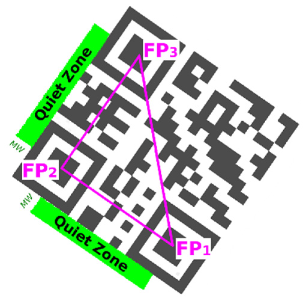
To verify the quiet zone, we check if there are only white points in the rectangular area of binary image which is parallel to line segments defined by FP1–FP2 and FP2–FP3 (Figure 8). For fast inspection of line points we use Bresenham’s line algorithm [28].
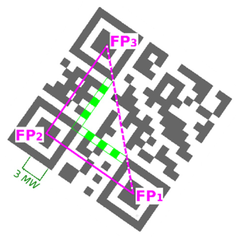
To verify timing patterns inside the QR Code, we examine the rectangular area between inner corners of finder patterns (Figure 9). We count the number of white and black points in the binary image and we calculate average length LAVG of white and black line segments and its standard deviation LSTDDEV. The timing pattern is expected to satisfy the following conditions:
3.4. QR Code Bounding Box
Vertexes of triangle FP1–FP2–FP3 are centroids of three finder patterns. Then this triangle is extended to the triangle P1–P2–P3, where arms of the triangle go through border modules of the QR Code (Figure 10). For example, the shift of FP3 to P3 in direction defined by vector (FP1, FP3) can be expressed as:
where MW is module width.
4. The Proposed Method
Identification of perspective distortion of the QR Code and determination of the position of the 4th corner point of the QR Code.
In the case of perspective (projective) distorted QR Codes, we need 4 points to set-up perspective transformation from a source square to destination quadrilateral [29]. The 3 corner points P1, P2, P3 have been identified using 3 finder patterns of the QR Code. Now the position of the 4th corner point P4 must be determined.
4.1. Alternative A—Evaluation of the Edge Projections
A QR Code is a 2D matrix and inner structure of the QR Code forms a chessboard-like structure. That means the individual modules create edges that are perpendicular to each other. It can be said that the optimal position of the point P4 is such, where the vertical and horizontal edge projections reach the largest standard deviation. We assume that at the optimal position of the point P4, both horizontal and vertical edges will be in alignment and thus their projections will show significant local maxima (amplitudes), which will alternate with significantly lower (up to zero) values. In the following, we propose an iterative algorithm to gradually improve the position of point P4 in order to find the optimal boundary of the QR Code. Algorithm can be defined by these steps:
Start with an initial estimate of the position of the point P4, which is calculated as the intersection of lines parallel to P2–P3 and P2–P1, so that points P1–P2–P3–P4 form a parallelogram (Figure 11 shows the starting position of the P4 point for various distorted QR Codes). Then start moving (shifting) the point P4 first vertically in the direction P4–P3 (Figure 12) and then horizontally in the direction P4–P1. The initial size of the shift step is for QR Codes with modules greater than 2 points set to 2 points, otherwise it is set to 1 point (the smaller the QR Code module is, the smaller the step is also).
For each shift of point P4, from the transformed region IT of the grayscale image, defined by points P1–P2–P3–P4, determine the image of horizontal edges IHE (the horizontal edge is calculated as the difference between the brightness of the current point at coordinates (x, y) and the point on the previous line at coordinates (x, y−1): ) and the horizontal projection (sum of absolute values) of these edges in the horizontal direction . For the vector PHE calculate the standard deviation (the score).
If the standard deviation (score) increases, then proceed in the selected direction, otherwise if the score has decreased during the last two steps, go back 2 steps (to the position with the highest score) and change the direction of the shift to the opposite. Repeat step 2.
If there is no increase even after the change of direction, return to the position of the point P4 with the highest score and reduce the shift step to ½ and repeat steps 3 and 4 (to refine the position of the P4 point).
Just as the optimal position of the point P4 in the vertical direction was searched using horizontal edges and horizontal projection (Figure 12), in the same way look for its optimal position in the horizontal direction using vertical edges. and vertical projection of edges .
(Note: to compute edge image, i.e., the derivate of grayscale image, we have tested also other derivate masks like Prewitt operator [−1, 0, +1] and non-local maxima suppression, but experimental results were not significantly better, therefore we stayed on simple difference [−1,+1], which is computationally most effective.)
In Figure 12 we see that by gradually moving the point P4 upwards to the point P3 (and thus to a more precise delineation of the QR Code), the standard deviation increases in each step and the horizontal projection of the horizontal edges has more pronounced local maxima, which are alternated by more pronounced minima.
As the above mentioned method (Alternative A) is sensitive (especially for small QR Codes with a module size up to 3 points) to the precise alignment of boundary lines P1–P2 resp. P2–P3 with the outer edges of the QR Code, it is necessary to refine the positions of these points. This can be achieved using the same approach (by evaluation of edge projections) and by moving the points P1 and P3 (Figure 13a) and then the lines P1–P2 and P2–P3 (Figure 13b) separately, while working with the projections of the edges in a narrow region of the image around the lines given by points P1–P2 and P2–P3 respectively.
Another alternative way to refine the initial position of corner points P1, P2, P3 uses edge projections in the narrow area of the outer frame of the finder pattern and shifts the corner points to the middle between the local minimum (represents white-black transition on the outer edge of the finder pattern frame) and the local maximum (represents black-white transition on the inner edge of the finder pattern frame) of edge projections. Horizontal projections of horizontal edges in the OH area are used for centering in the vertical axis and vertical projections of vertical edges in the OV area are used for centering in the horizontal axis (Figure 14).
After refining the positions of points P1, P2, P3, we look for the optimal position of point P4 as described in Section 4.1.
Identification of QR Code Distortion by Edge Orientation Analysis
Before the aforementioned method (Alternative A) it is possible to add one more step in which the orientation (directions) of significant edges in a QR Code is analyzed. According this analysis it is possible to identify perspective or cylindrical distortion of the QR Code and shift the initial position of the 4th point P4. (this rough determination of the initial position will allow us to reduce the number of steps required to find the optimal position of point P4 in Alternative A as well as to identify the cylindrical distortion. For QR Codes that are cylindrically distorted, Alternative A is not suitable because the perspective transformation is not sufficient to remove this type of deformation).
First, the image of the horizontal edges is analyzed (Figure 15b) and then the image of the vertical edges is analyzed also. The edge images are calculated for the sub-region of the grayscale image, which is defined by points P1–P2–P3–P4 (Figure 15a). For edge images the following steps are performed:
Suppress weak edge points in the edge images that have gradient less than the specified threshold (<20) and which do not represent local maxima. In the image of horizontal edges, the point d(x, y) is considered to be a local maximum if: d(x,y − 1) < d(x,y) > d(x,y + 1) and in the image of vertical edges if: d(x − 1,y) < d(x,y) > d(x + 1,y).
Connect adjacent strong edge points into continuous regions. For each contiguous region calculate the region descriptor: raw moments of zero to second order: M00 (area), M10, M01, M20, M11, M02 (Equation (7)).
where x, y are coordinates of strong edge point in the edge image IE.
Filter out insignificant regions (short edges) which have area M00 less than 3 times the estimated size of the module MW (Equations (3) and (4)). Continue to work only with significant regions (edges) (Figure 15c).
Divide the edge image horizontally and vertically into thirds. Classify each region into one of these thirds, based on the location of the centroid of each individual region. Centroid C of the region is calculated according to Equation (8). For each third calculate the average angle from the angles of the individual regions, which are classified into the given third. The angle (orientation) α of the region is also calculated from the moments (Equation (9)).
where μ are central moments of second order, which can be calculated from raw moments M.
Evaluate the average angles of regions in individual thirds.
Divide the image of horizontal edges horizontally into thirds and also the image of vertical edges vertically into thirds. If the average angle in the individual thirds gradually decreases or increases, i.e.,
or , where α1 is average angle in 1st third, α2 is average angle in 2nd third and α3 is average angle in 3rd third.
It is then a perspective-distorted QR Code and the position of point P4 can be shifted (either vertically in the case of analysis of horizontal edges or horizontally in the case of analysis of vertical edges) by:
, where l represents the width in the case of the image of horizontal edges and the height of the image in the case of the image of vertical edges.
Divide the image of the horizontal edges vertically into thirds and mark the average angle in the left third as β1 and the average angle in the right third as β3. If the angles β1 and β3 have opposite signs and their difference is above a defined threshold, then this indicates a cylindrical distortion in the y-axis. Similarly, we identify the cylindrical distortion in the x-axis by dividing the image of the vertical edges horizontally into thirds and comparing the angles in the upper and lower thirds.
4.2. Alternative B—Evaluation the Overlap of the Boundary Line
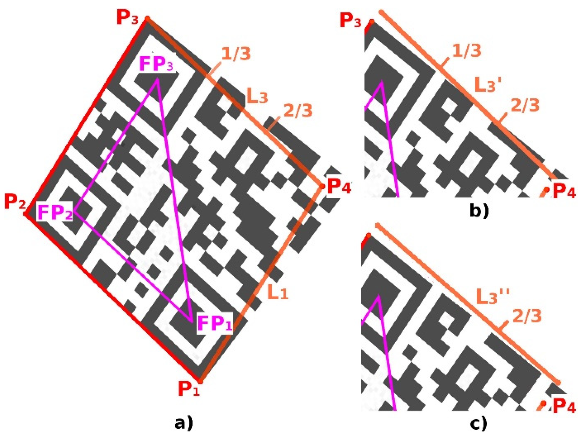
Another method (Alternative B) how to find the optimal position of the 4th corner point P4 is based on moving the boundary lines P3–P4 and P1–P4 and evaluating the overlap of the boundary lines with a QR Code (Figure 16).
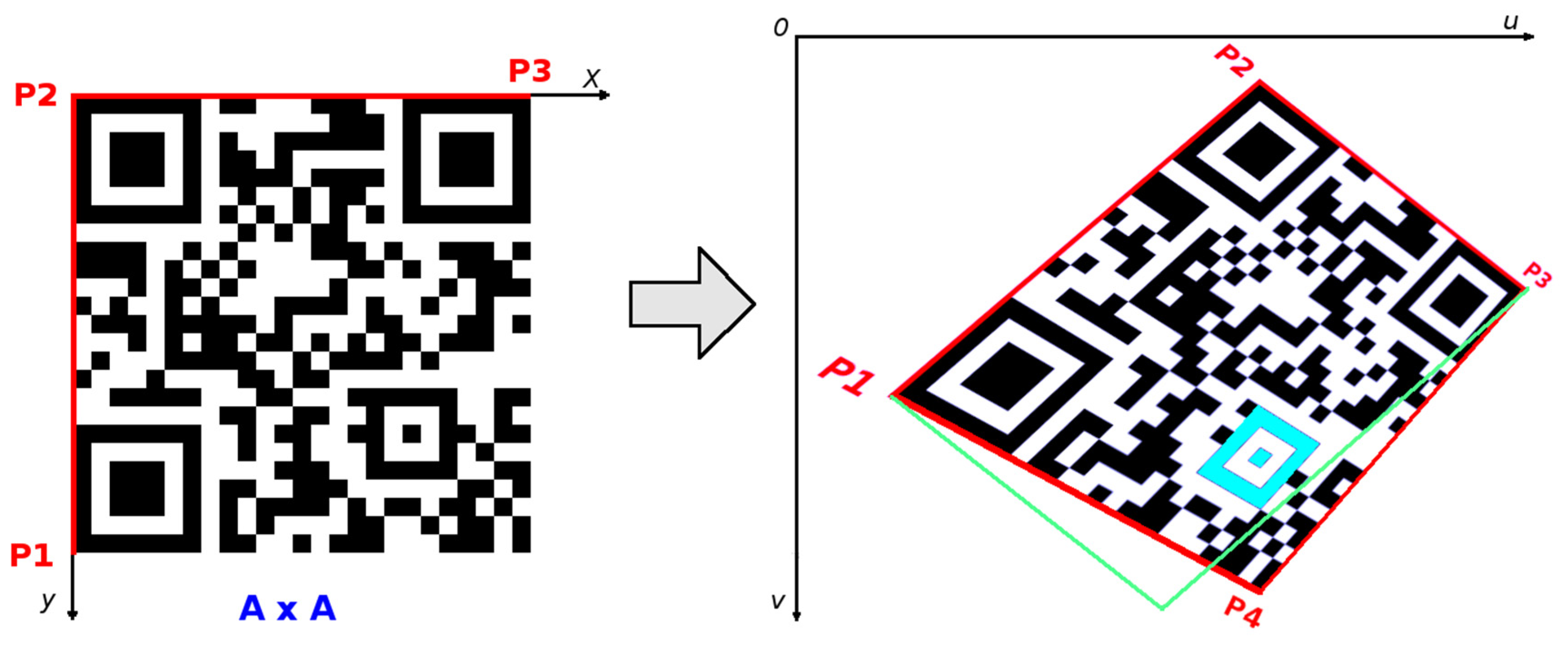
Once we have identified the position of the 4th point, P4, we can set-up perspective transformation from the source square domain representing an ideal QR Code to the quadrilateral destination representing a real QR Code in the image (Figure 17).
Using the following equations [29]:
, , where coefficients can be computed from coordinates of points P1(u1,v1), P2(u2, v2), P3(u3, v3), P4(u4, v4) as:
4.3. Decoding the QR Code
To successfully decode a QR Code, the precise location of all four corner points which form the bounding quadrilateral, must be done. Once perspective transformation is set up, we can map image points from this quadrilateral into square binary matrix. Dark modules become binary 1 and light modules become binary 0. This binary matrix is the input of a deterministic process that decodes the data stored in the QR Code. If the QR Code is only perspective distorted, then by applying a perspective transformation we get an image of a square QR Code, where its modules are also squares of the same size (Figure 17). In this case, creating the binary matrix is straightforward because it is enough to take the middle points of the modules, which decide whether the module is dark or light (Figure 18). If the modules are larger, we can also consider the average value of several adjacent points around the middle point. Whether a point is classified as dark or light depends on the local threshold value. We divide the whole area of the QR Code into 9 tiles (3 × 3) and for each tile we calculate its threshold value as the grayscale intensity average. Then the local threshold value is determined by bilinear interpolation of the thresholds of adjacent tiles.
If the deformation of the QR Code cannot be sufficiently restored only by inverse perspective transformation, for example if a cylindrical distortion is added to the perspective distortion, then the module sizes of the QR Code are not constant (Figure 19). In this case we have to adapt the positions of the middle points to the changing sizes of the modules. Again, we can apply the principle of edge projections when local maxima determine the edges of the modules and distances between two adjacent local maxima gives the size of the current module in the examined row or column. The middle points are then placed in the centre between adjacent local maxima. In the results we refer to this technique as “Dynamic grid”.
5. Results
The method mentioned above was tested on a test set consisting of 286 samples of QR Codes. The testing set contained 20 synthetic QR Codes of various sizes and rotations, 86 QR Codes from Internet images and 180 QR Codes from a specific manufacturing environment. The samples of the test codes are in Figure 20.
In Table 1 and Figure 21 there are our results compared against competitive QR Code decoding software (open-source and also commercial). In the table, there are the numbers of successfully recognized/decoded QR Codes out of a total of 286 codes.
Our method successfully localized all QR Codes, but failed to decode one sample. This sample was a QR Code placed on a bottle, so that the QR Code was perspective- and also cylindrically distorted. How to handle this kind of combined distortion is a challenge for our future research. Lay et al. [36] proposed a parametric cylindrical surface model for rectification of QR Codes printed on cylinders.
As the most of the competitive QR Code decoders are closed source solutions we cannot compare their and our detection algorithms in detail. For this reason, we have performed black-box testing only (using default settings). There does not exists standardized published QR Code testing datasets to compare the results of our method against the results of other previously published methods. Our testing dataset is published online together with this article under “Supplementary Material”.
In Table 2 is compared time consumption of individual solutions depending on the resolution of the input image and the number of QR Codes in one image (the table includes only open-source software that we could test on the same hardware with CPU i5-4590 3.3GHz; our solution was implemented in Free Pascal without using any optimized computer vision libraries).
6. Conclusions
We have proposed and tested a precise and fast method for the location of perspective-distorted 2D QR Codes in arbitrary images under various lighting conditions. This method is suitable for localization of single or multiple QR Codes in low-resolution images as well as for real time processing. The proposed methods use typical position detection patterns of QR Codes so-called finder patterns to identify three corners of QR Codes in an image. For distorted QR Codes perspective transformation must be set-up. The optimal position of the fourth corner of the QR Code is determined by analyzing the direction of horizontal and vertical edges and by maximizing the standard deviation of horizontal and vertical projections of these edges. Prerequisites of our method are the existence of intact finder patterns and quiet zones around a QR Code.
The novelty of our method lies in the way the bounding box of a QR Code is determined, especially for perspective-distorted QR Codes and how variable-sized modules are handled.
This method was validated on the testing set consisting of synthetic and also real world samples and it was compared with competitive solutions. The experimental results show that our method has a great detection rate. Unlike other articles, we consider a QR Code to be successfully recognized only if it is also decoded, not just localized. Precise localization is a necessary but not sufficient condition for successful decoding.
Supplementary Materials
The following are available online at https://0-www-mdpi-com.brum.beds.ac.uk/2313-433X/6/7/67/s1, one ZIP file contains images of testing dataset of QR Codes used to test our proposed algorithms.
Author Contributions
Conceptualization, methodology, software, writing—original draft preparation, L.K.; validation, writing—review and editing, visualization, E.P.; supervision, project administration, funding acquisition, P.B.; All authors have read and agreed to the published version of the manuscript.
Funding
This research was funded by VEGA project 1/0019/20: Accurate calculations, modeling and simulation of emerging surfaces based on the physical causes of machining surfaces and surfaces created by additive technologies in the conditions of machine and robotic machining.
Acknowledgments
The contribution is sponsored by the project.
Conflicts of Interest
The authors declare no conflict of interest. The funders had no role in the design of the study, in the collection, analyses, or interpretation of data; in the writing of the manuscript; or in the decision to publish the results.
References
- Frankovsky, P.; Pastor, M.; Dominik, L.; Kicko, M.; Trebuna, P.; Hroncova, D.; Kelemen, M. Wheeled Mobile Robot in Structured Environment. In Proceedings of the 12th International Conference ELEKTRO, Mikulov, Czech Republic, 21–23 May 2018. [Google Scholar]
- Božek, P.; Nikitin, Y.; Bezák, P.; Fedorko, G.; Fabian, M. Increasing the production system productivity using inertial navigation. Manuf. Technol. 2015, 15, 274–278. [Google Scholar]
- Denso Wave Incorporated: What Is a QR Code? Available online: http://www.qrcode.com/en/about/ (accessed on 6 September 2018).
- Denso Wave Incorporated: History of QR Code. Available online: http://www.qrcode.com/en/history/ (accessed on 6 September 2018).
- Lin, J.-A.; Fuh, C.-S. 2D Barcode Image Decoding. Math. Probl. Eng. 2013, 1–10. [Google Scholar] [CrossRef]
- Li, S.; Shang, J.; Duan, Z.; Huang, J. Fast detection method of quick response code based on run-length coding. IET Image Process. 2018, 12, 546–551. [Google Scholar] [CrossRef]
- Belussi, L.F.F.; Hirata, N.S.T. Fast component-based QR Code detection in arbitrarily acquired images. J. Math. Imaging Vis. 2013. [Google Scholar] [CrossRef]
- Bodnár, P.; Nyúl, L.G. Improved QR Code Localization Using Boosted Cascade of Weak Classifiers. Acta Cybern. 2015, 22, 21–33. [Google Scholar] [CrossRef] [Green Version]
- Tribak, H.; Zaz, Y. QR Code Recognition based on Principal Components Analysis Method. Int. J. Adv. Comput. Sci. Appl. 2017, 8. [Google Scholar] [CrossRef] [Green Version]
- Tribak, H.; Zaz, Y. QR Code Patterns Localization based on Hu Invariant Moments. Int. J. Adv. Comput. Sci. Appl. 2017. [Google Scholar] [CrossRef] [Green Version]
- Ciążyński, K.; Fabijańska, A. Detection of QR-Codes in Digital Images Based on Histogram Similarity. Image Process. Commun. 2015, 20, 41–48. [Google Scholar] [CrossRef] [Green Version]
- Szentandrási, I.; Herout, A.; Dubská, M. Fast Detection and Recognition of QR Codes in High-Resolution Images. In Proceedings of the 28th Spring Conference on Computer Graphics; ACM: New York, NY, USA, 2012. [Google Scholar]
- Gaur, P.; Tiwari, S. Recognition of 2D Barcode Images Using Edge Detection and Morphological Operation. Int. J. Comput. Sci. Mob. Comput. IJCSMC 2014, 3, 1277–1282. [Google Scholar]
- Kong, S. QR Code Image Correction based on Corner Detection and Convex Hull Algorithm. J. Multimed. 2013, 8, 662–668. [Google Scholar] [CrossRef]
- Sun, A.; Sun, Y.; Liu, C. The QR-Code Reorganization in Illegible Snapshots Taken by Mobile Phones. In Proceedings of the 2007 International Conference on Computational Science and its Applications (ICCSA 2007), Kuala Lumpur, Malaysia, 26–39 August 2007; pp. 532–538. [Google Scholar]
- Hansen, D.K.; Nasrollahi, K.; Rasmussen, C.B.; Moeslund, T.B. Real-Time Barcode Detection and Classification using Deep Learning. IJCCI 2017, 1, 321–327. [Google Scholar]
- Zharkov, A.; Zagaynov, I. Universal Barcode Detector via Semantic Segmentation. In Proceedings of the 2019 International Conference on Document Analysis and Recognition (ICDAR), Sydney, Australia, 20–25 September 2019; pp. 837–843. [Google Scholar]
- Chou, T.-H.; Ho, C.-S.; Kuo, Y.-F. QR Code Detection Using Convolutional Neural Networks. In Proceedings of the 2015 International Conference on Advanced Robotics and Intelligent Systems (ARIS), Taipei, Taiwan, 29–31 May 2015; pp. 1–5. [Google Scholar] [CrossRef]
- Kurniawan, W.C.; Okumura, H.; Muladi; Handayani, A.N. An Improvement on QR Code Limit Angle Detection using Convolution Neural Network. In Proceedings of the 2019 International Conference on Electrical, Electronics and Information Engineering (ICEEIE), Denpasar, Bali, Indonesia, 3 October 2019; pp. 234–238. [Google Scholar] [CrossRef]
- Lopez-Rincon, O.; Starostenko, O.; Alarcon-Aquino, V.; Galan-Hernandez, J.C. Binary Large Object-Based Approach for QR Code Detection in Uncontrolled Environments. J. Electr. Comput. Eng. 2017, 2, 1–15. [Google Scholar] [CrossRef] [Green Version]
- Niblack, W. An Introduction to Digital Image Processing; Prentice Hall: Englewood Cliffs, NJ, USA, 1986. [Google Scholar]
- Sauvola, J.; Pietikäinen, M. Adaptive document image binarization. Pattern Recognit. 2020, 33, 225–236. [Google Scholar] [CrossRef] [Green Version]
- Bradley, D.; Roth, G. Adaptive thresholding using the integral image. J. Graph. Tools 2007, 12, 13–21. [Google Scholar] [CrossRef]
- Sulaiman, A.; Omar, K.; Nasrudin, M.F. Degraded Historical Document Binarization: A Review on Issues, Challenges, Techniques, and Future Directions. J. Imaging 2019, 5, 48. [Google Scholar] [CrossRef] [Green Version]
- Calvo-Zaragoza, J.; Gallego, A.-J. A selectional auto-encoder approach for document image binarization. Pattern Recognit. 2019, 86, 37–47. [Google Scholar] [CrossRef] [Green Version]
- Rosenfeld, A.; Pfaltz, J. Sequential Operations in Digital Picture Processing. J. ACM 1966, 13, 471–494. [Google Scholar] [CrossRef]
- Bailey, D.G.; Klaiber, M.J. Zig-Zag Based Single-Pass Connected Components Analysis. J. Imaging 2019, 5, 45. [Google Scholar] [CrossRef] [Green Version]
- Bresenham, J.E. Algorithm for computer control of a digital plotter. IBM Syst. J. 1965, 4, 25–30. [Google Scholar] [CrossRef]
- Heckbert, P. Fundamentals of Texture Mapping and Image Warping. Available online: http://www2.eecs.berkeley.edu/Pubs/TechRpts/1989/5504.html (accessed on 6 September 2018).
- Google: ZXing (“Zebra Crossing”) Barcode Scanning Library for Java, Android. Available online: https://github.com/zxing (accessed on 22 September 2018).
- Beer, D. Quirc-QR Decoder Library. Available online: https://github.com/dlbeer/quirc (accessed on 22 September 2018).
- Leadtools: QR Code SDK Technology. Available online: http://demo.leadtools.com/JavaScript/Barcode/index.html (accessed on 22 September 2018).
- Inlite Research Inc.: Barcode Reader SDK. Available online: https://online-barcode-reader.inliteresearch.com (accessed on 22 September 2018).
- Terriberry, T.B. ZBar Barcode Reader. Available online: http://zbar.sourceforge.net (accessed on 22 September 2018).
- Dynamsoft: Barcode Reader SDK. Available online: https://www.dynamsoft.com/Products/Dynamic-Barcode-Reader.aspx (accessed on 22 September 2018).
- Lay, K.; Wang, L.; Wang, C. Rectification of QR-Code Images Using the Parametric Cylindrical Surface Model. In Proceedings of the International Symposium on Next-Generation Electronics (ISNE), Taipei, Taiwan, 4–6 May 2015; pp. 1–5. [Google Scholar]
- Karrach, L.; Pivarčiová, E.; Nikitin, Y.R. Comparing the impact of different cameras and image resolution to recognize the data matrix codes. J. Electr. Eng. 2018, 69, 286–292. [Google Scholar] [CrossRef] [Green Version]
Figure 1.
Version 2: 25 × 25 modules Quick Response (QR) Code.

Figure 2.
The flow chart of the proposed algorithm.
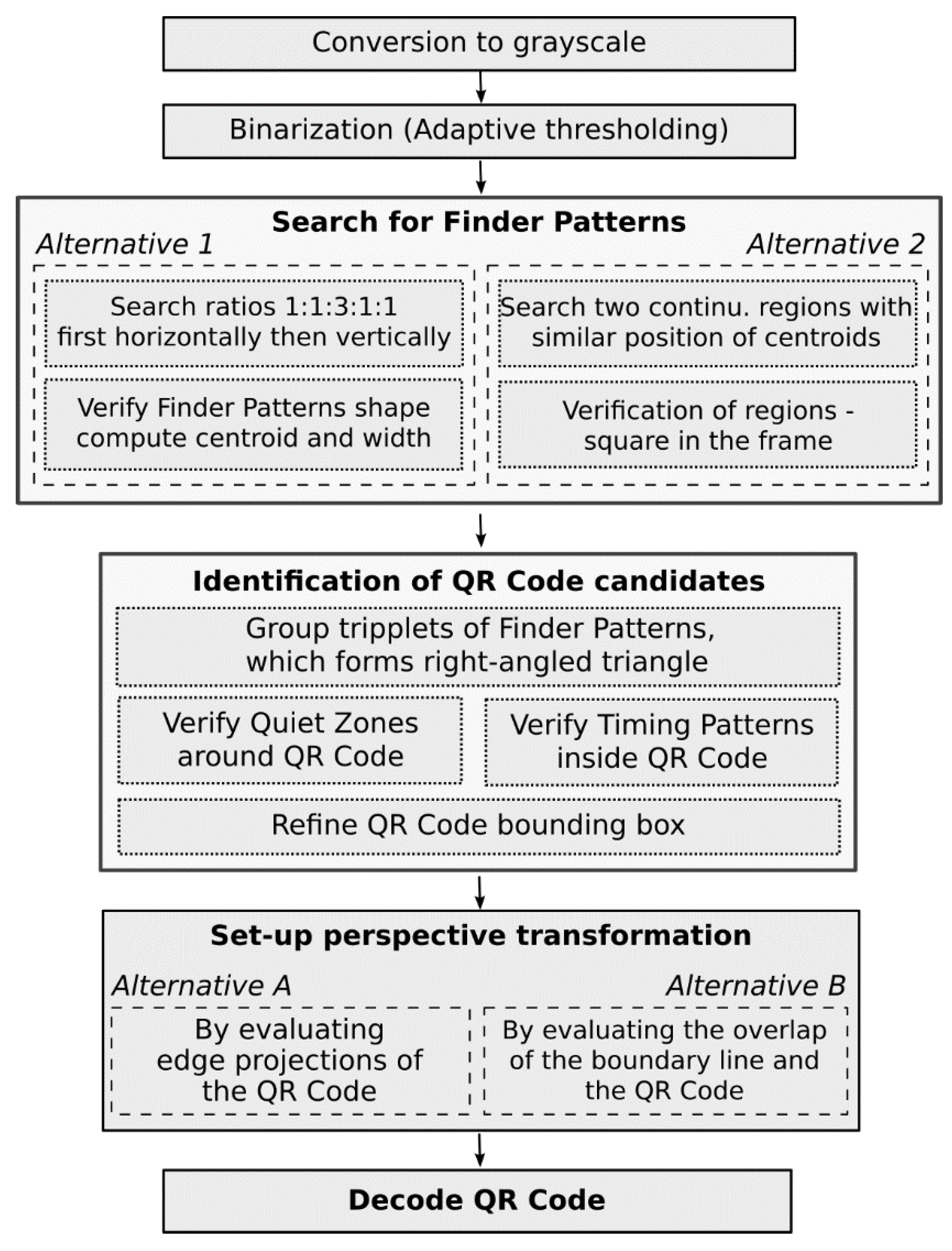
Figure 3.
The finder pattern.

Figure 4.
Finder pattern candidate matching 1:1:3:1:1.
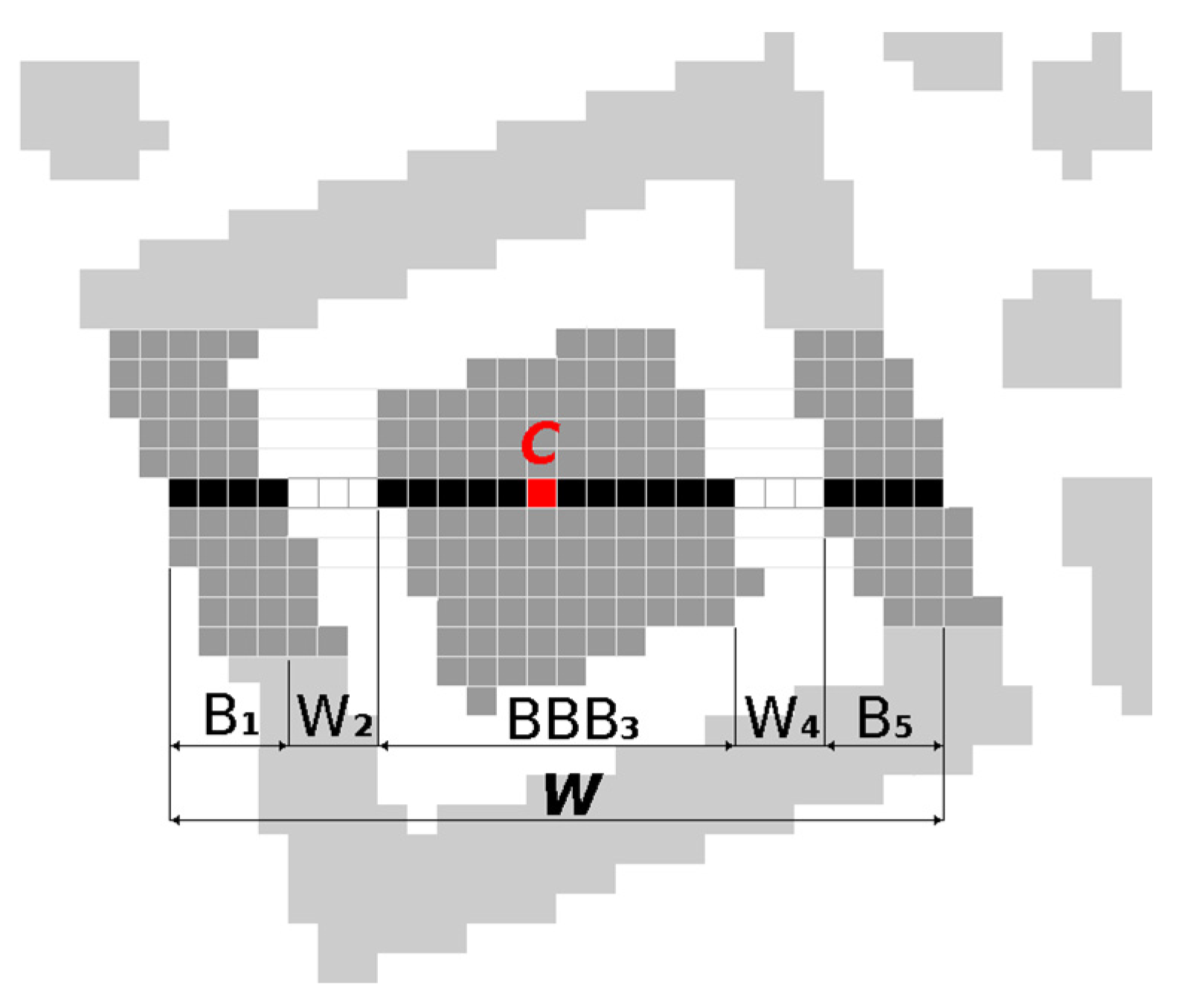
Figure 5.
Finder pattern candidate matching 1:1:3:1:1 in both axes.

Figure 6.
Connected components of the finder pattern candidate.
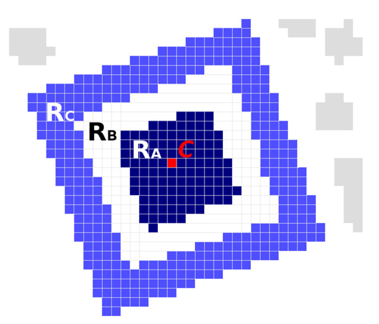
Figure 7.
QR Code candidates.

Figure 8.
Quiet zones around QR Code.

Figure 9.
Timing patterns inside a QR Code.

Figure 10.
Bounding box.
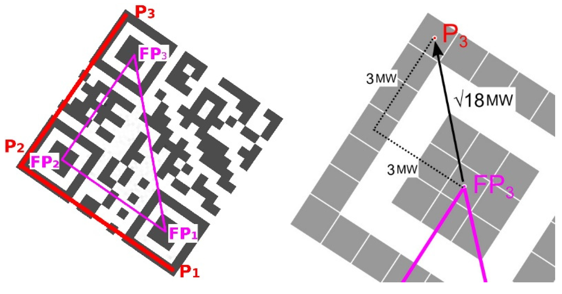
Figure 11.
Initial estimate of position of 4th point P4. (a) undistorted QR Code; (b) skewed QR Code; (c,d) perspective distorted QR Codes.
Figure 11.
Initial estimate of position of 4th point P4. (a) undistorted QR Code; (b) skewed QR Code; (c,d) perspective distorted QR Codes.

Figure 12.
Identification of perspective deformation of QR Code: (a) QR Code; (b) horizontal edges; (c) horizontal projection of horizontal edges.
Figure 12.
Identification of perspective deformation of QR Code: (a) QR Code; (b) horizontal edges; (c) horizontal projection of horizontal edges.

Figure 13.
Refining the position of the corner points of the QR Code (alternative 1). (a) refining the position of the points P1 and P3; (b) refining the position of the lines P1–P2 and P2–P3.
Figure 13.
Refining the position of the corner points of the QR Code (alternative 1). (a) refining the position of the points P1 and P3; (b) refining the position of the lines P1–P2 and P2–P3.

Figure 14.
Refining of the position of the corner points of the QR Code (alternative 2). (a) areas of the finder pattern where edge projections are evaluated; (b) local extrema in edge projections.
Figure 14.
Refining of the position of the corner points of the QR Code (alternative 2). (a) areas of the finder pattern where edge projections are evaluated; (b) local extrema in edge projections.
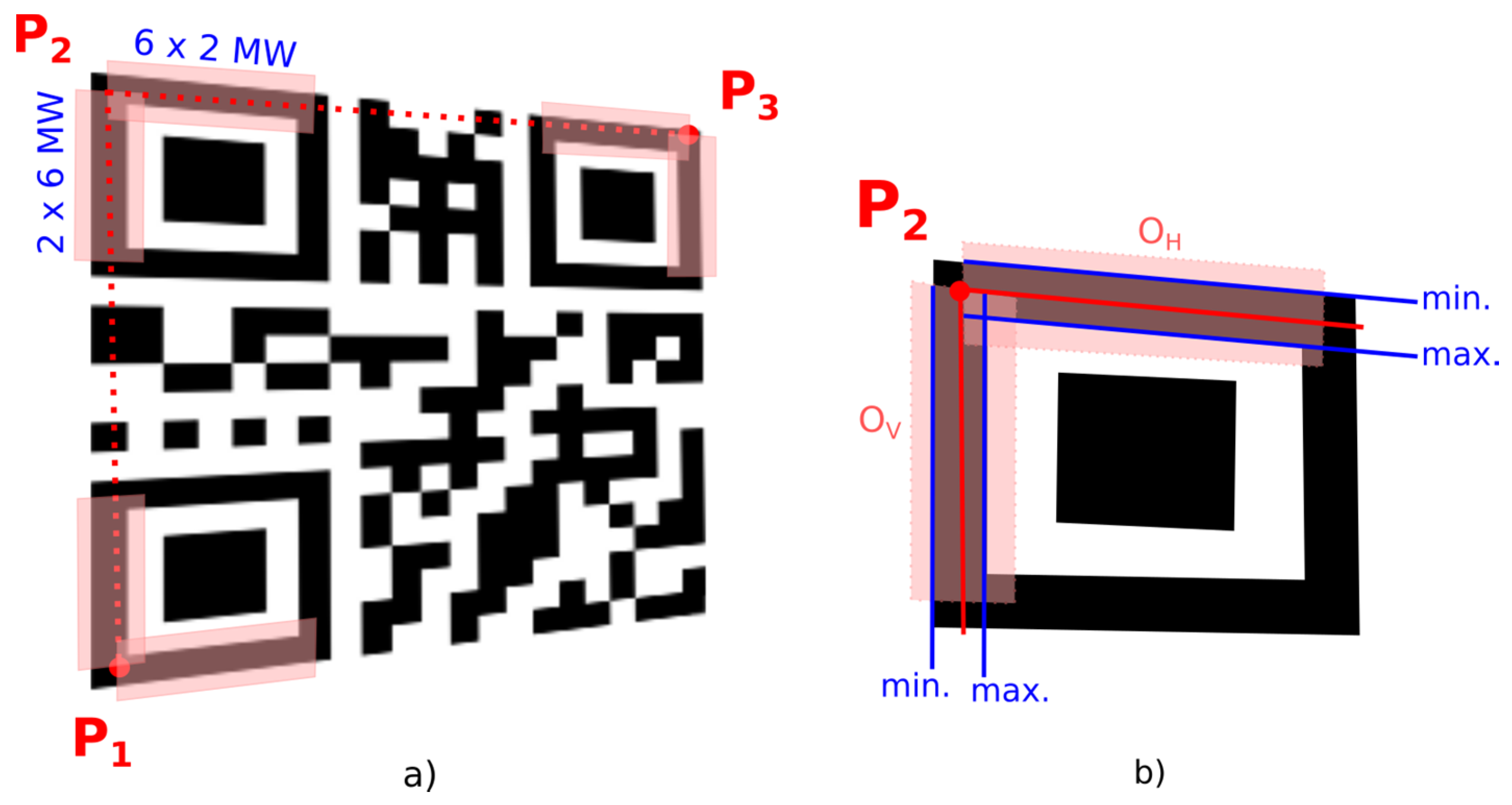
Figure 15.
Identification of QR Code distortion by edge orientation analysis: (a) QR Code; (b) horizontal edges image; (c) significant edges.
Figure 15.
Identification of QR Code distortion by edge orientation analysis: (a) QR Code; (b) horizontal edges image; (c) significant edges.

Figure 16.
Perspective distortion. (a) initial position of the point P4 and lines L1, L3; (b) first shift of the line L3; (c) second shift of the line L3.
Figure 16.
Perspective distortion. (a) initial position of the point P4 and lines L1, L3; (b) first shift of the line L3; (c) second shift of the line L3.

Figure 17.
Perspective transformation.

Figure 18.
Mapping of the QR Code into the binary matrix.

Figure 19.
Variable-sized modules.

Figure 20.
Testing samples: (a) synthetic; (b) Internet; (c) manufacturing.

Figure 21.
Our results compared with competitive solutions.
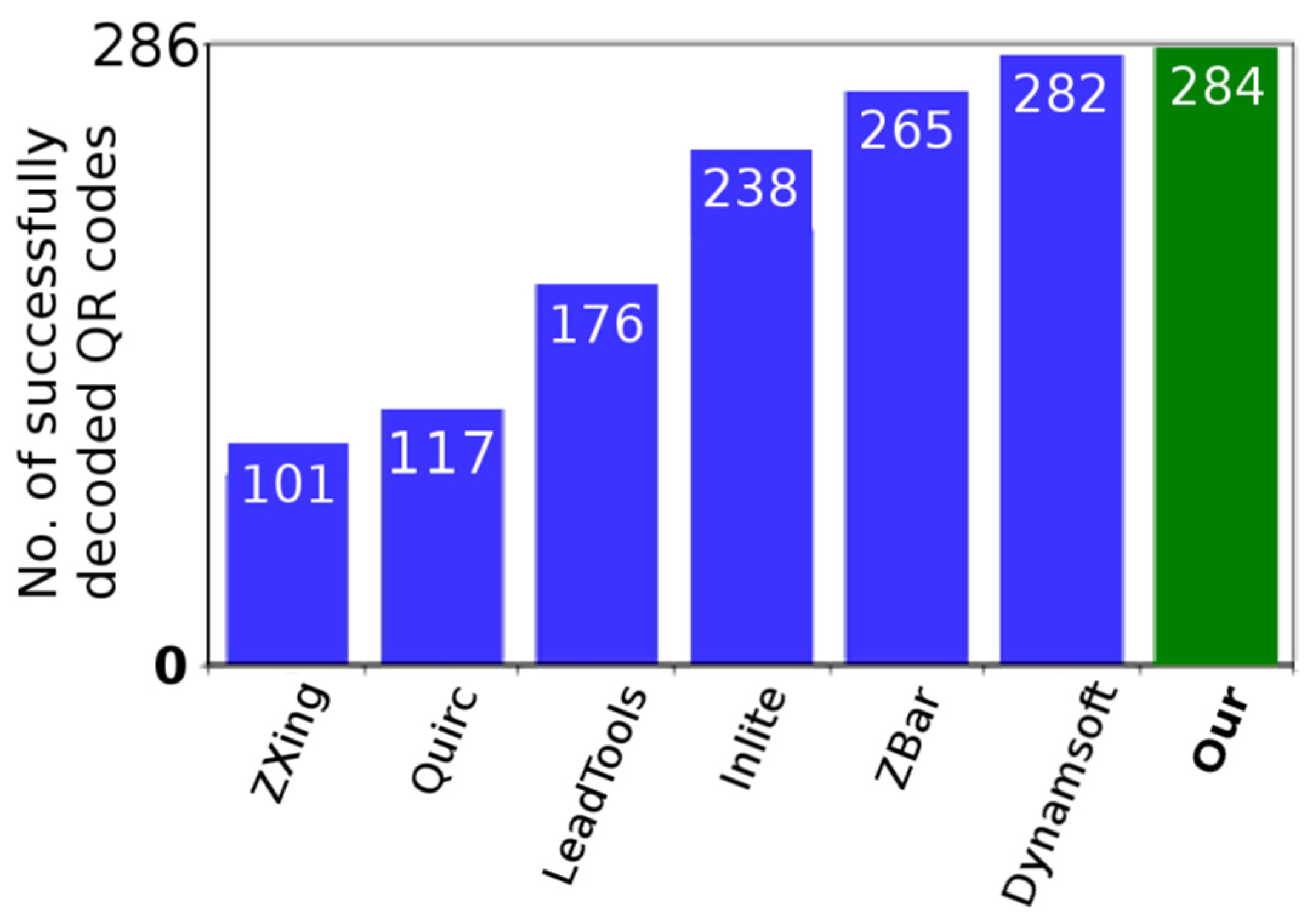
Figure 22.
Other types of 2D codes: (a) micro QR Code; (b) data matrix code.


Table 1.
Our results compared with competitive solutions.
| Software | Samples (a) | Samples (b) | Samples (c) |
|---|---|---|---|
| Google ZXing (open-source) [30] | 1 | 70 | 30 |
| Quirc (open-source) [31] | 12 | 66 | 39 |
| LEADTOOLS QR Code SDK [32] | 7 | 69 | 100 |
| Inlite Barcode Reader SDK [33] | 18 | 79 | 141 |
| ZBar (open-source) [34] | 20 | 78 | 167 |
| Dynamsoft Barcode Reader SDK [35] | 20 | 84 | 178 |
| Our—Alternative 1.A, Dynamic grid | 20 | 85 | 180 |
| Our—Alternative 2.A, Dynamic grid | 20 | 85 | 179 |
Table 2.
Approximate time consumption of tested software.
| Software | 1024 × 768 | 1296 × 960 | 2592 × 1920 | ||||
|---|---|---|---|---|---|---|---|
| 1 code | 10 codes | 1 code | 10 codes | 1 code | 10 codes | 50 codes | |
| Quirc (open-source) | 10 ms | 34 ms | 15 ms | 37 ms | 66 ms | 130 ms | 430 ms |
| ZBar (open-source) | 48 ms | 96 ms | 76 ms | 124 ms | 338 ms | 396 ms | 1781 ms |
| Our—Alternative 1.A | 17 ms | 77 ms | 23 ms | 83 ms | 74 ms | 135 ms | 426 ms |
| Our—Alternative 2.A | 17 ms | 79 ms | 22 ms | 83 ms | 69 ms | 129 ms | 414 ms |
© 2020 by the authors. Licensee MDPI, Basel, Switzerland. This article is an open access article distributed under the terms and conditions of the Creative Commons Attribution (CC BY) license (http://creativecommons.org/licenses/by/4.0/).
Share and Cite
MDPI and ACS Style
Karrach, L.; Pivarčiová, E.; Božek, P. Identification of QR Code Perspective Distortion Based on Edge Directions and Edge Projections Analysis. J. Imaging 2020, 6, 67. https://0-doi-org.brum.beds.ac.uk/10.3390/jimaging6070067
AMA Style
Karrach L, Pivarčiová E, Božek P. Identification of QR Code Perspective Distortion Based on Edge Directions and Edge Projections Analysis. Journal of Imaging. 2020; 6(7):67. https://0-doi-org.brum.beds.ac.uk/10.3390/jimaging6070067
Chicago/Turabian StyleKarrach, Ladislav, Elena Pivarčiová, and Pavol Božek. 2020. "Identification of QR Code Perspective Distortion Based on Edge Directions and Edge Projections Analysis" Journal of Imaging 6, no. 7: 67. https://0-doi-org.brum.beds.ac.uk/10.3390/jimaging6070067
Note that from the first issue of 2016, this journal uses article numbers instead of page numbers. See further details here.