On Computational Aspects of Krawtchouk Polynomials for High Orders
by
 , , and
Basheera M. Mahmmod
1,‡ ,
,
Alaa M. Abdul-Hadi
1,‡,
Sadiq H. Abdulhussain
1,*,†,‡ and
Aseel Hussien
2,‡ 1
Department of Computer Engineering, University of Baghdad, Baghdad 10071, Iraq
2
Department of Computer Science, Liverpool John Moores University, Liverpool L3 3AF, UK
*
Author to whom correspondence should be addressed.
†
Current address: Department of Computer Engineering, University of Baghdad, Baghdad 10071, Iraq.
‡
These authors contributed equally to this work.
J. Imaging 2020, 6(8), 81; https://0-doi-org.brum.beds.ac.uk/10.3390/jimaging6080081
Submission received: 2 July 2020
/
Revised: 8 August 2020
/
Accepted: 11 August 2020
/
Published: 13 August 2020
(This article belongs to the Special Issue Mathematical Models of Visual Perception and Biology with Applications to Images Processing and Computer Vision)
Abstract
:Discrete Krawtchouk polynomials are widely utilized in different fields for their remarkable characteristics, specifically, the localization property. Discrete orthogonal moments are utilized as a feature descriptor for images and video frames in computer vision applications. In this paper, we present a new method for computing discrete Krawtchouk polynomial coefficients swiftly and efficiently. The presented method proposes a new initial value that does not tend to be zero as the polynomial size increases. In addition, a combination of the existing recurrence relations is presented which are in the n- and x-directions. The utilized recurrence relations are developed to reduce the computational cost. The proposed method computes approximately 12.5% of the polynomial coefficients, and then symmetry relations are employed to compute the rest of the polynomial coefficients. The proposed method is evaluated against existing methods in terms of computational cost and maximum size can be generated. In addition, a reconstruction error analysis for image is performed using the proposed method for large signal sizes. The evaluation shows that the proposed method outperforms other existing methods.
1. Introduction
Discrete orthogonal moments, simply moments, are utilized as a feature descriptor in several fields such as signal processing and computer vision [1]. Moments, mathematically, are formed from the projection of a signal on the discrete orthogonal polynomial basis to ensure non-redundancy of the feature set [2,3]. Tchebichef, Hahn, Charlier, and Krawtchouk polynomials are types of polynomials that are used to generate discrete moments. Amongst them, Krawtchouk can express an image locally [2]. Beside, discrete Krawtchouk polynomials (DKPs) have been combined with other polynomials to enhance the performance of the resulted polynomial by adding the localization property of the DKP such as discrete Krawtchouk–Tchebichef polynomials [4], Squared Tchebichef–Krawtchouk polynomials [5], and Squared Krawtchouk–Tchebichef polynomials [6]. Krawtchouk polynomials and its hybrid forms have been utilized in different applications such as speech enhancement [7], shot boundary detection [8,9], and information hiding [10]. The DKP has a parameter (p) that controls the shifting direction of the features [11]. The parameter p at 0.5 has a special case because it equally divides the moment plane into four portions and makes the feature extraction more simple than other values of parameter p.
Many efforts have been conducted to compute the DKP coefficients (DKPCs) using three-term recurrence algorithm (TTRA). The TTRA is employed as a replacement to the hypergeometric series and gamma functions because these functions are time-consuming. Yap et al. [11] presented TTRA in the n-direction to compute DKPCs. Koekkoek et al. [12] presented the TTRA in the x-direction to generate DKPCs. However, when the image size becomes large, DKPCs shows instability because of the numerical propagation errors. The method presented in [13] shows that a reduction in the computation of recurrence times is the key to reduce the numerical error. However, the existing methods suffer from the problem of initial value which tends to be zero as the polynomial-size increases [13]. To overcome this problem, this paper proposes a new method to compute the DKPCs efficiently and swiftly. The proposed method investigated a new location to compute the initial value which is then used to compute the rest of the DKPCs. Based on the location of the initial value, a new TTRA is presented to compute the DKPCs with a reduction in the computation of polynomials coefficients.
2. Preliminaries
In this section, the definitions DKPs are presented as well as the recurrence relation which are employed in the proposed method. The n-th order of the weighted and normalized DKP is defined as follows [12]:
where denotes the hypergeometric series and is defined as:
where represents the rising factorial defined as:
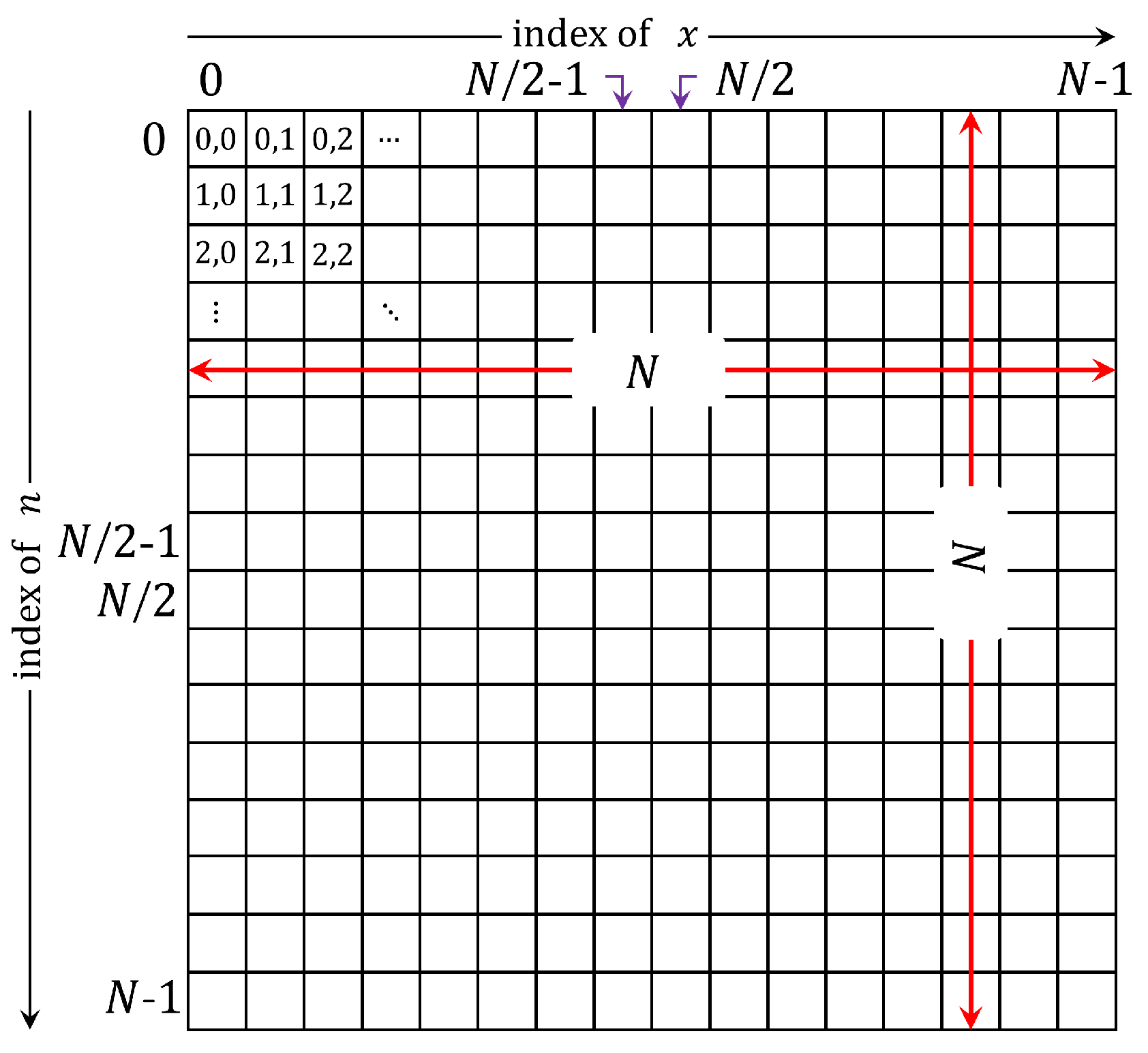
DKPs are generally a two-dimensional array with three parameters as shown in Figure 1, which are: (1) the size of the array , (2) the polynomial order parameter (n), and (3) the polynomial index parameter (x).
The computation of the DKPCs using Equation (1) is considered computationally cost due to the usage of hypergeometric and gamma functions. Therefore, the three-term recurrence algorithm (TTRA) is employed for computing the DKPCs [14]. Two types of TTRAs are introduced: TTRAs in the x- and n-directions.
In this algorithm, the polynomial coefficients are computed by employing the coefficients at the orders and .
In this algorithm, the DKPCs are computed by considering the values of the coefficients at the indices and .
3. Proposed Recurrence Algorithm
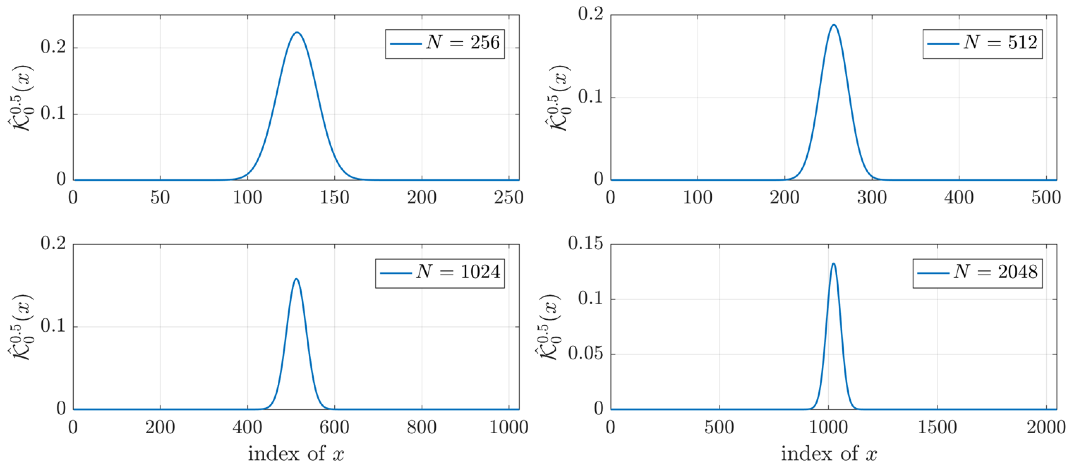
Computing the initial value is considered important and impacts the values of DKPCs. Previous algorithms failed to compute DKP for high order because the location where initial value computed goes to zero which in turn makes the rest of the values polynomial zero out. Thus, unlike the existing algorithm which considers as the initial values. Figure 2 shows the results of the for different values of polynomial size. From Figure 2, it is clear that when , the values of becomes very small and in several environments considered zero. On the other hand, the value of at always large values.
The proposed initial value is computed at and . From Equation (1), the initial value can be written as follows:
The problem with Equation (8) is that the gamma function, , produces very large numbers and produces infinity in several environments such as MATALB and python. To overcome this problem, natural logarithmic gamma function, , can be utilized. Thus, Equation (8) can be written as follows:
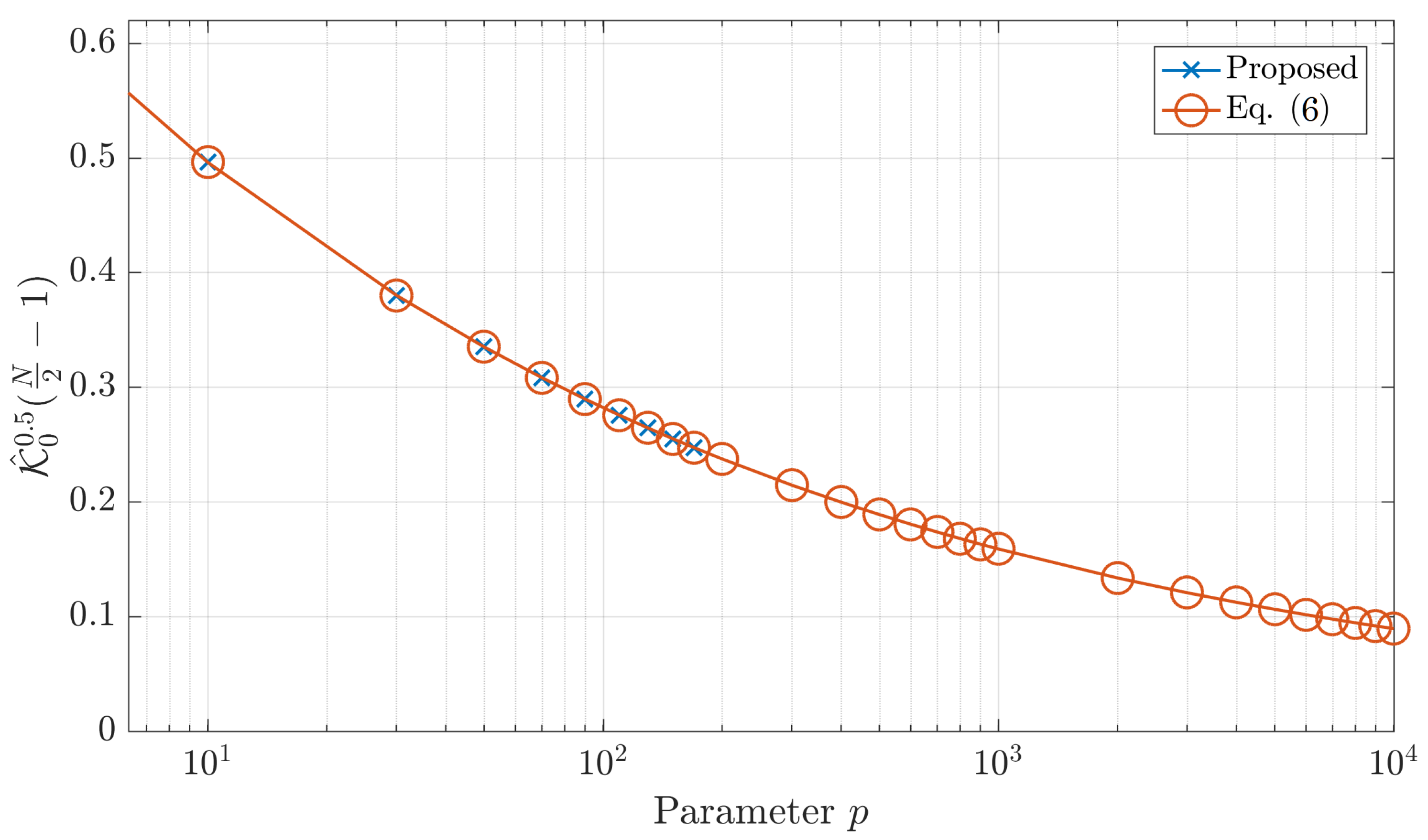
where represents the natural logarithmic function represents the logarithmic gamma function. The maximum limit of each function is presented in Figure 3 which clearly shows that the proposed formula can compute the initial values for a wide range of polynomial size.
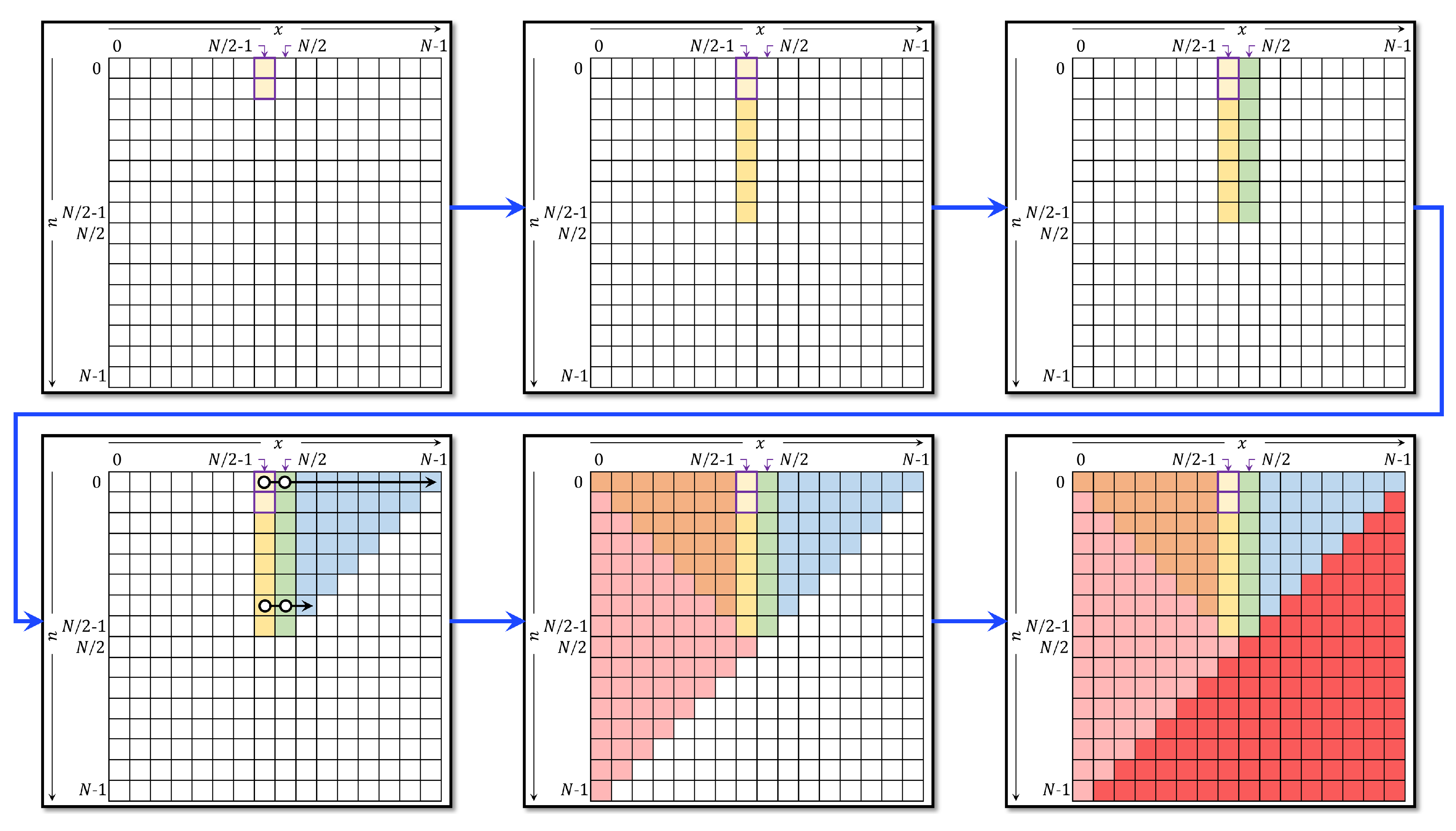
The plane of the DKP is partitioned as shown in Figure 4. After finding a computable initial value, the value of the coefficient at and need to be computed. The coefficient of is computed as follows:
It is noteworthy mentioning that the plane of the DKP is partitioned as shown in Figure 4. After computing the four coefficients, the TTRA in the n-direction can be employed to compute the values in the range and . However, a reduced form of the TTRA in the n-direction is presented and used. The reduced form of the TTRA is defined as:
To compute the values in the range and , the following symmetry relation is utilized [13]:
Next, the coefficients of the DKP are computed in the range and (region K11 in Figure 4) using the proposed reduced form in the x-direction TTRA as follows:
The coefficient in the range and (region K12 in Figure 4) is computed using symmetry relation [13] as follows:
The coefficients in the range and (region K2 in Figure 4) are computed using the following symmetry relation [13]:
The coefficients in the range and (region K3 in Figure 4) are computed using the following symmetry relation [13]:
The steps of the method are depicted in Figure 5 and can be summarized as follows:
- The Initial value is computed using Equation (9).
- The value of is computed from using Equation (10).
- The first set of initial used for TTRA is computed in the range of and using Equation (11).
- The first set of initial used for TTRA is computed in the range of and using Equation (12).
- The modified recurrence algorithm, Equation (13), is used to compute the values of the coefficients in the range and . It should be noted that, for each x, when and , the recurrence relation is terminated and n is increased by 1.
4. Performance Evaluation of the Proposed Method
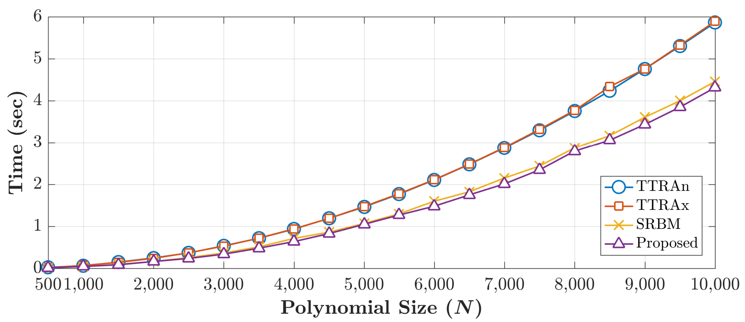
A comparison with the existing methods is performed based on two criteria: computation cost and maximum generated size. A comparison of computation time is performed for different polynomials size. The existing algorithms are the TTRA in the n-direction (TTRAn) [11], TTRA in the x-direction (TTRAx) [12], and symmetry relation-based method (SRBM) [13]. The execution time is carried out using Krawtchouk parameter and different DKP sizes. Figure 6 shows the execution time required for each algorithm to generate DKPCs with a size of . For each method, average execution time for 10 runs is reported in Figure 6.
From Figure 6, it can be noticed that the execution times TTRAn [11] and TTRAx [12] are approximately identical because both of the algorithms are computing 50% of coefficients using the recurrence algorithm. TTRAn employs Equation (4) and TTRAx employs Equation (6). The rest of the coefficients are computed using similarity relation. For SRBM [13], only 12.5% of the coefficients are computed; thus, it shows less execution time when compared to TTRAn and TTRAx.
Obviously, in the proposed method, the average execution time to generate DKPCs is less than existing methods. This achievement is due to: (1) the proposed method computed only 12.5% of the DKPCs, and (2) a reduced complexity forms of the existing recurrence relations are introduced (Equations (11) and (13)). To affirm the results of the proposed algorithm, the improvement ratio of the execution time is measured. The improvement of the proposed algorithm to SRBM is ∼3.7%; while the improvement ratio over the TTRAn and TTRAx is ∼30%. Accordingly, it can be inferred that the proposed algorithm outperforms the existing methods in terms of the execution time.
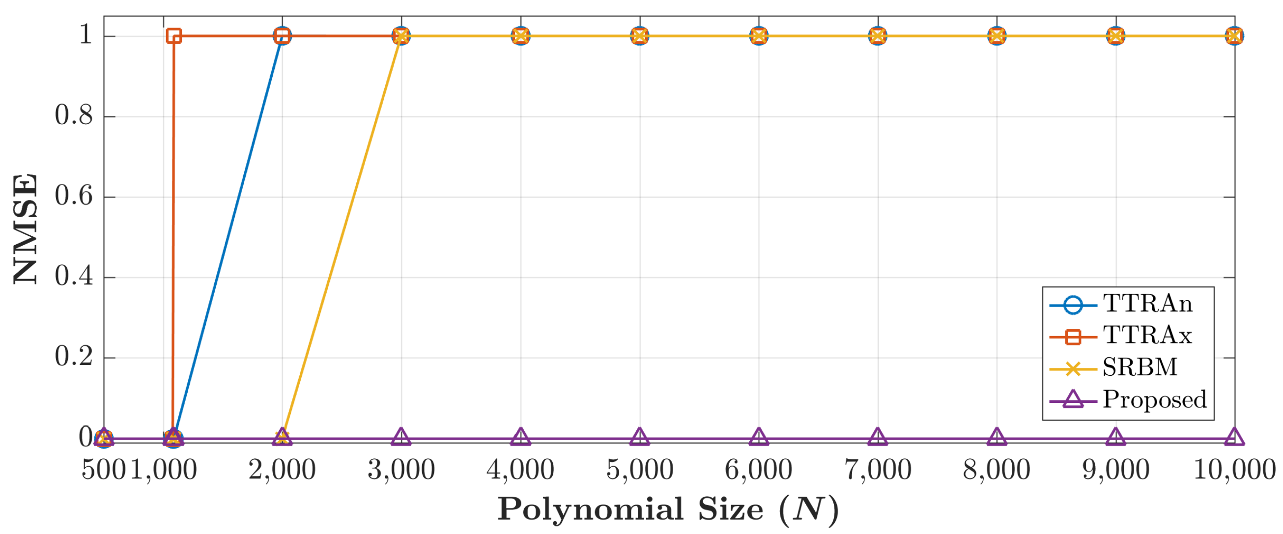
The proposed method is also evaluated in terms of maximum size can be generated and compared to that of the existing methods. For each method, the maximum size is found using the procedure presented in [13]:
- A test image, , is used.
- The test image is resized to a small size ,
- DKP, , is generated with signal size and order of (),
- The moment, , is computed using ,
- The test image is then reconstructed back from the moment domain using ,
- The normalized mean square error (NMSE) is computed between and ,
- If the , the size of the image and DKP is increased by 2, i.e., and repeat step 1 to 7.
- If the , the maximum size can be generated by the polynomial is reached and reported.
- The maximum size considered in the experiment is set to 12,288.
where the NMSE is computed as follows:
Note that, the cameraman image is considered in the experiment as the test image. From the previous experiment, the maximum size of the TTRAn is 1090, TTRAx is 1080, SRBM is 2140, and for the proposed method is 12,288 (12K). The experiment reveals that the proposed method outperforms the existing method and the improvement factor is ∼5.7 times greater than SRBM and ∼11.3 times greater than TTRAn and TTRAx. To confirm the performance of the proposed algorithm, the reconstruction error in terms of the NMSE for all cases presented in Figure 6 are shown in Figure 7.
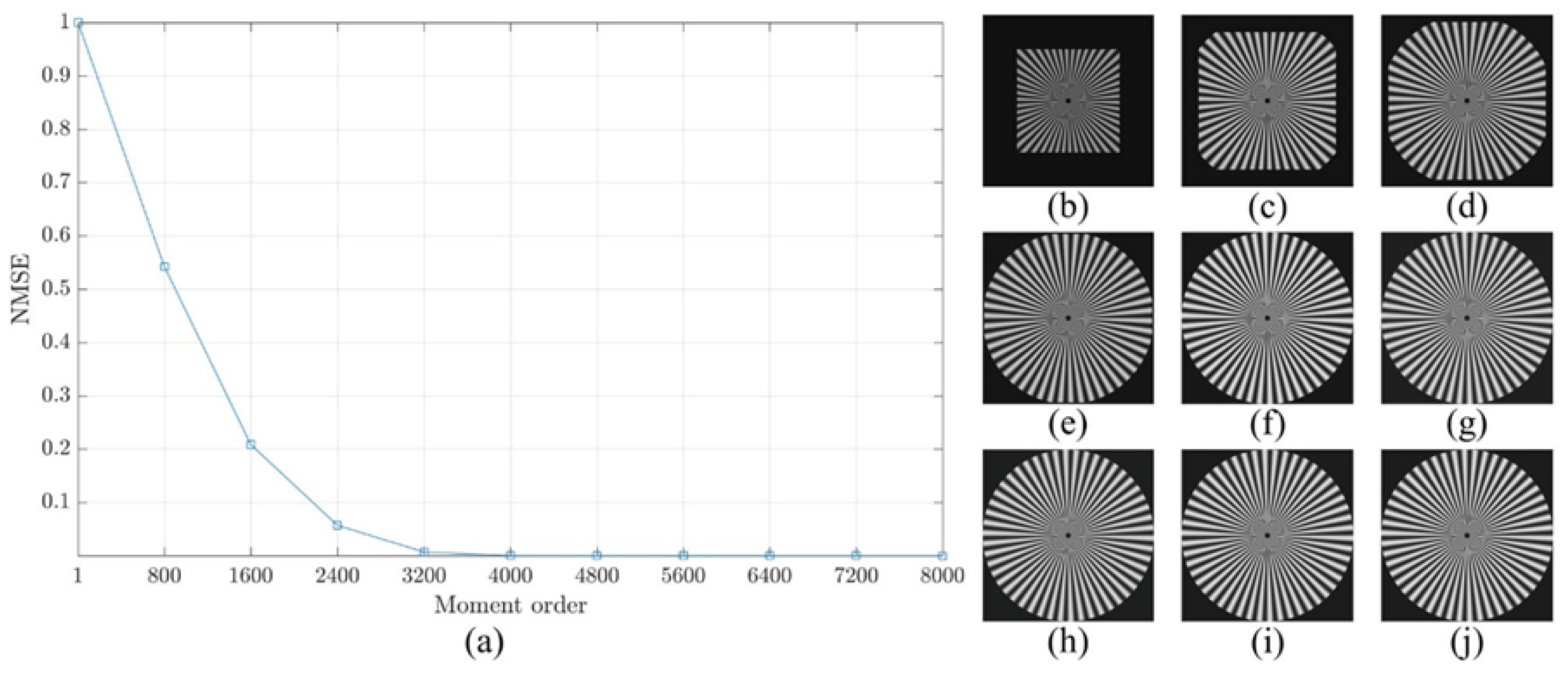
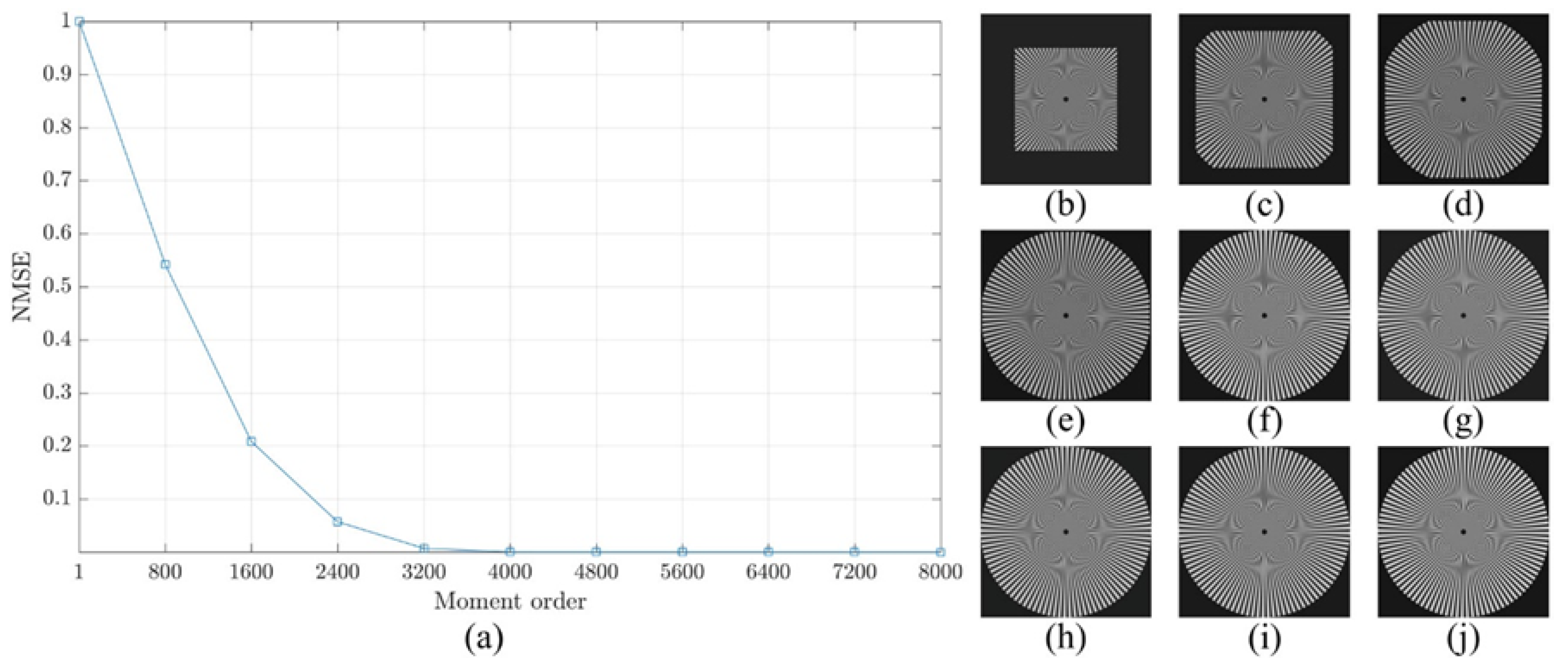
For more clarification regarding the ability of the proposed method, a reconstruction error analysis is performed for the proposed method to test its accuracy. The reconstruction error analysis is performed using a reconstruction error Sinusoidal Siemens star which is utilized to examine the resolution of optical systems and printers. Sinusoidal Siemens star involves of sinusoidal oscillations patterns in a polar coordinate system such that the spatial frequency varies for concentric circles of different sizes. The Sinusoidal Siemens star is defined as [15]:
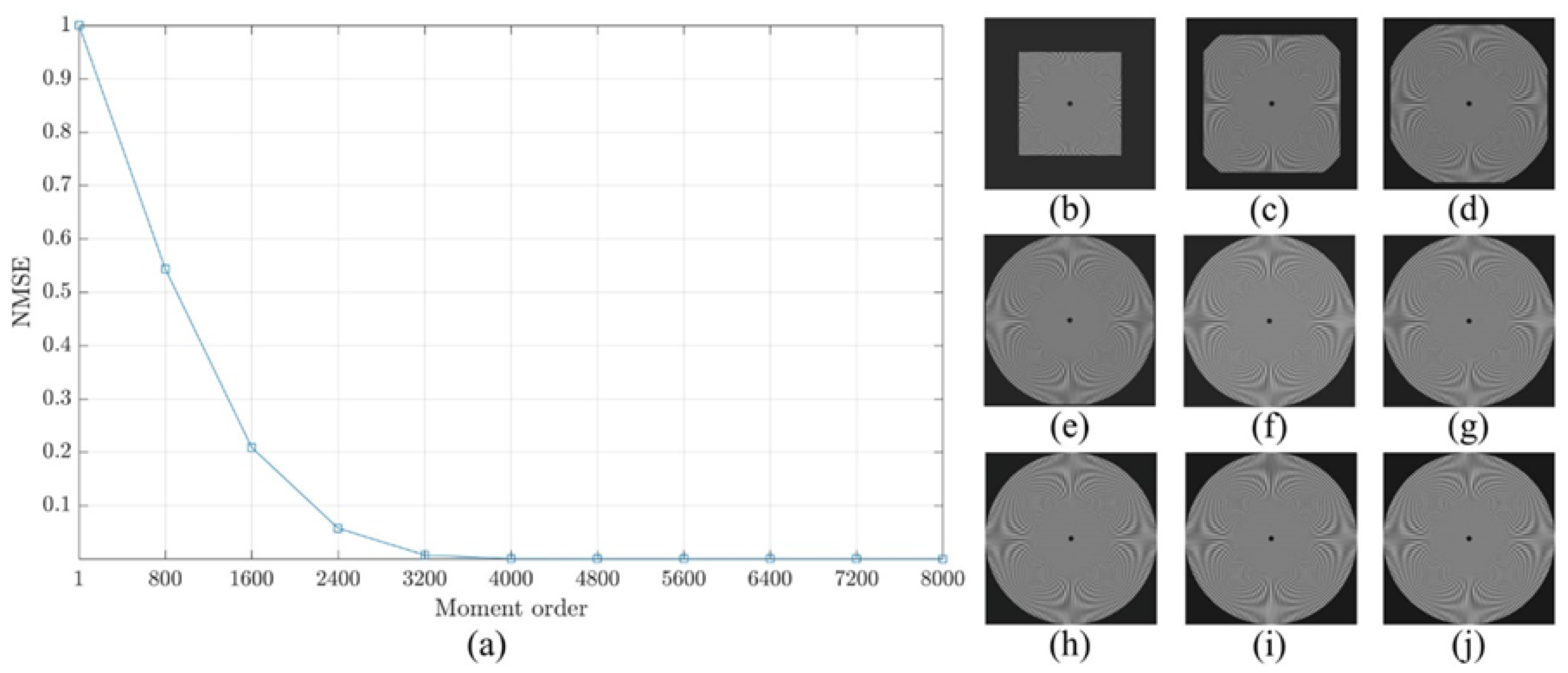
where I represent the intensity represented by a sinusoidal function with an angle . In addition, a, b, , and are the intensity mean, the intensity amplitude, the number of cycles, and the phase offset, respectively. Figure 8 shows Sinusoidal Siemens star with different values of number of cycles which are . In the experiment, the parameters of the sinusoidal Siemens star are considered as follows , , , and .
The reconstruction analysis using the proposed method is performed for an image with a size of . First, the image is transformed into the moment domain of the DKP. Then, the image is reconstructed using a limited number of moments. The number of moments is increased by a step of 800 until the image is fully reconstructed using the total number of moments. The obtained results are shown in Figure 9, Figure 10 and Figure 11. From the figures, it is clear that the proposed method is able to generate a stable DKP with high order. For instance, the image reconstruction analysis shows that the NMSE closes to zero when the moment order reaches , i.e., the DKP can represent the signal using only 50% of the moments; moreover, the spokes of sinusoidal Siemens star are never touched or overlap. This led to the proposed method to compute DKP has remarkable performance and satisfy the orthogonality condition without distortion.
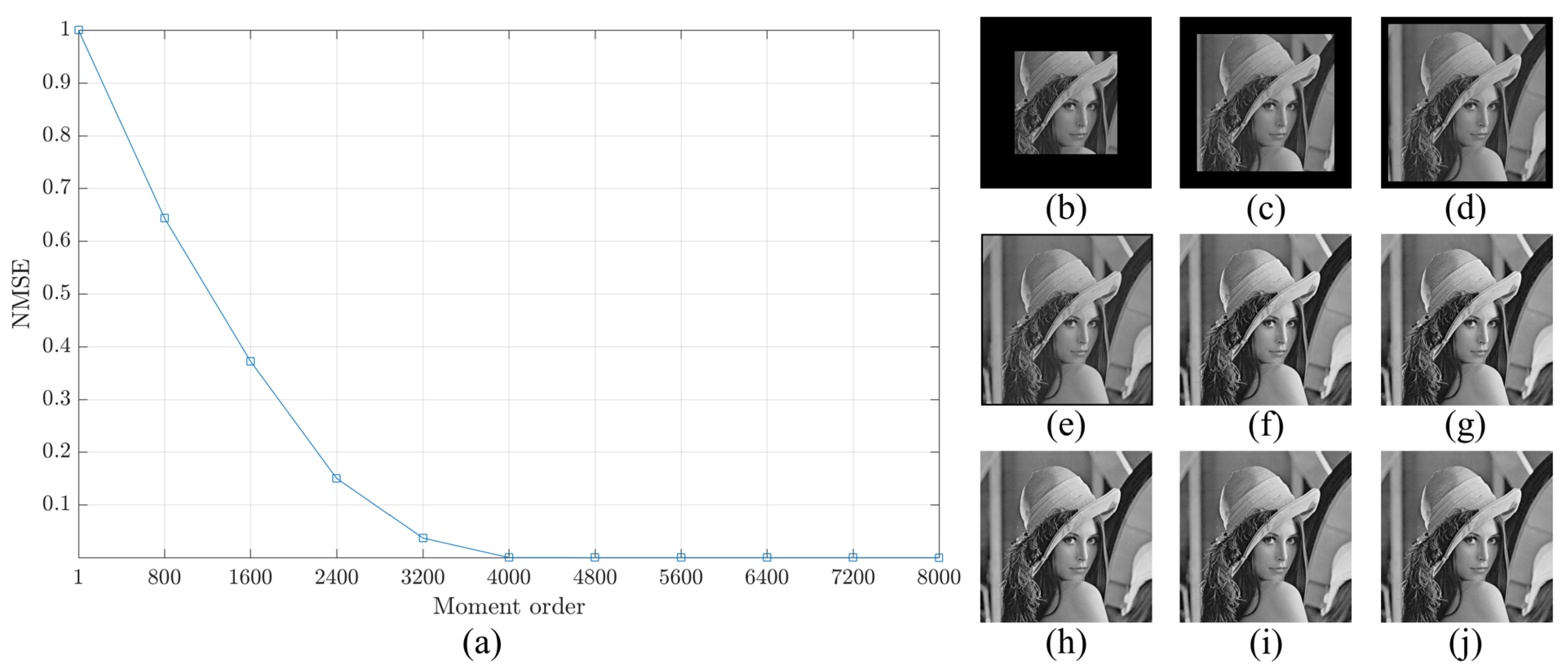
In addition to Sinusoidal Siemens star, the well known image of Lena is utilized for reconstruction analysis. The Lena image is resized to obtain Lena image with a size of . The same procedure for Sinusoidal Siemens is performed for Lena image. The result is shown in Figure 12. The result clearly confirm that the proposed method is able to generate a stable DKP with high order.
To sum up, the proposed method is able to compute DKP accurately and satisfy the orthogonality condition without distortion for large signal size and order.
5. Conclusions
This paper presents a new method for efficiently computing the DKPCs. The presented method is based on the combination of the existing recurrence methods as well as a new initial value formula with values not tend to zero. The initial values and the combined recurrence methods are utilized to compute the coefficients of the DKP in a specified portion. Then, the recurrence relations are employed to compute the rest coefficients of the DKP for other portions. The results show that the proposed method has significantly less computational cost when compared to the existing methods. In addition, the proposed method has the ability to minimize the propagation errors which in turn makes it able to generate DKP with high order and size of 12,288.
Author Contributions
These authors contributed equally to this work. S.H.A. conceived the ideas for this article; S.H.A., B.M.M., A.M.A.-H., and A.H. had detailed discussions about the contents, structure and organization of the manuscript; S.H.A., B.M.M., and A.M.A.-H. contributed to modifications, improvements commonly, responses to the review comments and manuscript revision. All authors have read and agreed to the published version of the manuscript.
Funding
This research received no external funding.
Acknowledgments
We would like express our heartfelt thanks to all of the anonymous reviewers for their efforts, valuable comments and suggestions. We would also like to acknowledge University of Baghdad for general support.
Conflicts of Interest
The authors declare no conflict of interest.
Abbreviations
The following abbreviations are used in this manuscript:
| DKP | discrete Krawtchouk polynomials |
| DKPC | discrete Krawtchouk polynomial Coefficient |
| TTRA | three-term recurrence algorithm |
| TTRAn | three-term recurrence algorithm in the n-direction |
| TTRAx | three-term recurrence algorithm in the x-direction |
| SRBM | symmetry relation-based method |
| NMSE | normalized mean square error |
References
- Camacho-Bello, C.; Rivera-Lopez, J.S. Some computational aspects of Tchebichef moments for higher orders. Pattern Recognit. Lett. 2018, 112, 332–339. [Google Scholar] [CrossRef]
- Akhmedova, F.; Liao, S. Face recognition using discrete orthogonal hahn moments. World Acad. Sci. Eng. Technol. Int. J. Comput. Electr. Autom. Control Inf. Eng. 2015, 9, 1550–1556. [Google Scholar]
- Abdul-Hadi, A.M.; Abdulhussain, S.H.; Mahmmod, B.M. On the computational aspects of Charlier polynomials. Cogent Eng. 2020, 7, 1763553. [Google Scholar] [CrossRef]
- Mahmmod, B.M.; bin Ramli, A.R.; Abdulhussain, S.H.; Al-Haddad, S.A.R.; Jassim, W.A. Signal compression and enhancement using a new orthogonal-polynomial-based discrete transform. IET Signal Process. 2018, 12, 129–142. [Google Scholar] [CrossRef]
- Idan, Z.N.; Abdulhussain, S.H.; Al-Haddad, S.A.R. A New separable moments based on Tchebichef– Krawtchouk polynomials. IEEE Access 2020, 8, 41013–41025. [Google Scholar] [CrossRef]
- Abdulhussain, S.H.; Ramli, A.R.; Mahmmod, B.M.; Saripan, M.I.; Al-Haddad, S.A.R.; Jassim, W.A. A new hybrid form of Krawtchouk and Tchebichef polynomials: Design and application. J. Math. Imaging Vis. 2019, 61, 555–570. [Google Scholar] [CrossRef]
- Mahmmod, B.M.; Ramli, A.R.; Baker, T.; Al-Obeidat, F.; Abdulhussain, S.H.; Jassim, W.A. Speech enhancement algorithm based on super-gaussian modeling and orthogonal polynomials. IEEE Access 2019, 7, 103485–103504. [Google Scholar] [CrossRef]
- Abdulhussain, S.H.; Rahman Ramli, A.; Mahmmod, B.M.; Iqbal Saripan, M.; Al-Haddad, S.; Baker, T.; Flayyih, W.N.; Jassim, W.A. A fast feature extraction algorithm for image and video processing. In Proceedings of the 2019 International Joint Conference on Neural Networks (IJCNN), Budapest, Hungary, 14–19 July 2019; IEEE: Piscataway, NJ, USA, 2019; pp. 1–8. [Google Scholar]
- Abdulhussain, S.H.; Al-Haddad, S.A.R.; Saripan, M.I.; Mahmmod, B.M.; Hussien, A. Fast temporal video segmentation based on Krawtchouk–Tchebichef moments. IEEE Access 2020, 8, 72347–72359. [Google Scholar] [CrossRef]
- Radeaf, H.S.; Mahmmod, B.M.; Abdulhussain, S.H.; Al-Jumaeily, D. A steganography based on orthogonal moments. In Proceedings of the International Conference on Information and Communication Technology—CICT ’19; ACM Press: New York, NY, USA, 2019; pp. 147–153. [Google Scholar]
- Yap, P.-T.; Paramesran, R.; Ong, S.-H. Image analysis by krawtchouk moments. IEEE Trans. Image Process. 2003, 12, 1367–1377. [Google Scholar] [PubMed] [Green Version]
- Koekoek, R.; Lesky, P.A.; Swarttouw, R.F. Hypergeometric Orthogonal Polynomials and Their Q-Analogues; Springer Science & Business Media: Berlin/Heidelberg, Germany, 2010. [Google Scholar]
- Abdulhussain, S.H.; Ramli, A.R.; Al-Haddad, S.A.R.; Mahmmod, B.M.; Jassim, W.A. Fast recursive computation of Krawtchouk polynomials. J. Math. Imaging Vis. 2018, 60, 285–303. [Google Scholar] [CrossRef]
- Zhu, H.; Liu, M.; Shu, H.; Zhang, H.; Luo, L. General form for obtaining discrete orthogonal moments. IET Image Process. 2010, 4, 335. [Google Scholar] [CrossRef]
- Birch, G.C.; Griffin, J.C. Sinusoidal Siemens star spatial frequency response measurement errors due to misidentified target centers. Opt. Eng. 2015, 54, 074104. [Google Scholar] [CrossRef]
Figure 1.
The 2D array parameters of DKPCs.

Figure 2.
Plot of for different values of polynomial size.

Figure 4.
The partitions of the DKP plane.
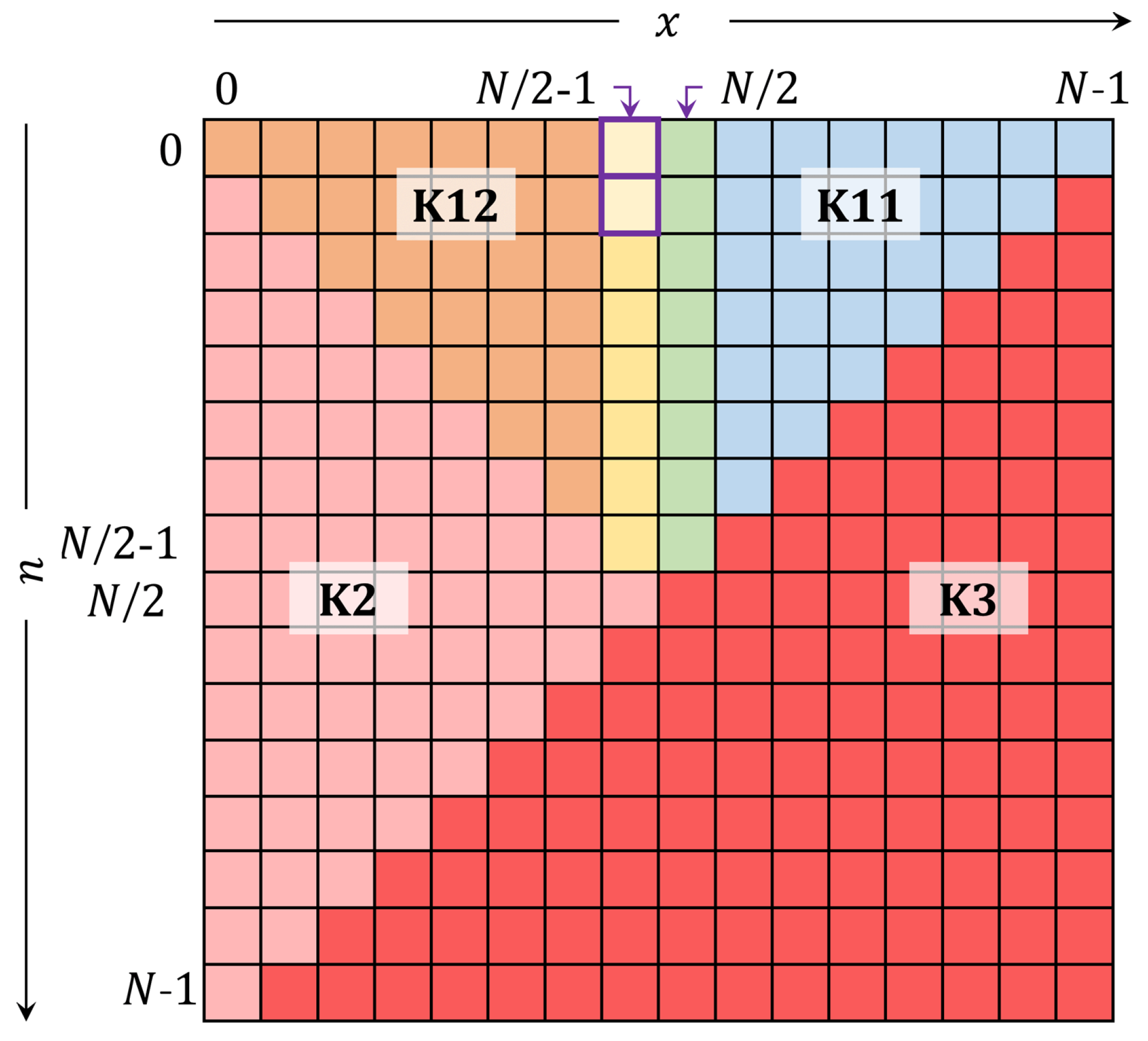
Figure 5.
The steps used to compute DKPCs using the proposed recurrence algorithm.

Figure 6.
Computation time of the proposed and existing methods.

Figure 7.
Reconstruction error of the proposed and existing methods.

Figure 8.
Sinusoidal Siemens star: (a) , (b) , (c) .

Figure 9.
Construction analysis for the proposed method using sinusoidal Siemens start with . (a) NMSE, image reconstructed using number of moment equal to (b) 800, (c) 1600, (d) 2400, (e) 3200, (f) 4000, (g) 4800, (h) 5600, (i) 6400, and (j) 7200.
Figure 9.
Construction analysis for the proposed method using sinusoidal Siemens start with . (a) NMSE, image reconstructed using number of moment equal to (b) 800, (c) 1600, (d) 2400, (e) 3200, (f) 4000, (g) 4800, (h) 5600, (i) 6400, and (j) 7200.

Figure 10.
Construction analysis for the proposed method using sinusoidal Siemens start with . (a) NMSE, image reconstructed using number of moment equal to (b) 800, (c) 1600, (d) 2400, (e) 3200, (f) 4000, (g) 4800, (h) 5600, (i) 6400, and (j) 7200.
Figure 10.
Construction analysis for the proposed method using sinusoidal Siemens start with . (a) NMSE, image reconstructed using number of moment equal to (b) 800, (c) 1600, (d) 2400, (e) 3200, (f) 4000, (g) 4800, (h) 5600, (i) 6400, and (j) 7200.

Figure 11.
Construction analysis for the proposed method using sinusoidal Siemens start with . (a) NMSE, image reconstructed using number of moment equal to (b) 800, (c) 1600, (d) 2400, (e) 3200, (f) 4000, (g) 4800, (h) 5600, (i) 6400, and (j) 7200.
Figure 11.
Construction analysis for the proposed method using sinusoidal Siemens start with . (a) NMSE, image reconstructed using number of moment equal to (b) 800, (c) 1600, (d) 2400, (e) 3200, (f) 4000, (g) 4800, (h) 5600, (i) 6400, and (j) 7200.

Figure 12.
Construction analysis for the proposed method using Lena image. (a) NMSE, image reconstructed using number of moment equal to (b) 800, (c) 1600, (d) 2400, (e) 3200, (f) 4000, (g) 4800, (h) 5600, (i) 6400, and (j) 7200.
Figure 12.
Construction analysis for the proposed method using Lena image. (a) NMSE, image reconstructed using number of moment equal to (b) 800, (c) 1600, (d) 2400, (e) 3200, (f) 4000, (g) 4800, (h) 5600, (i) 6400, and (j) 7200.

© 2020 by the authors. Licensee MDPI, Basel, Switzerland. This article is an open access article distributed under the terms and conditions of the Creative Commons Attribution (CC BY) license (http://creativecommons.org/licenses/by/4.0/).
Share and Cite
MDPI and ACS Style
Mahmmod, B.M.; Abdul-Hadi, A.M.; Abdulhussain, S.H.; Hussien, A. On Computational Aspects of Krawtchouk Polynomials for High Orders. J. Imaging 2020, 6, 81. https://0-doi-org.brum.beds.ac.uk/10.3390/jimaging6080081
AMA Style
Mahmmod BM, Abdul-Hadi AM, Abdulhussain SH, Hussien A. On Computational Aspects of Krawtchouk Polynomials for High Orders. Journal of Imaging. 2020; 6(8):81. https://0-doi-org.brum.beds.ac.uk/10.3390/jimaging6080081
Chicago/Turabian StyleMahmmod, Basheera M., Alaa M. Abdul-Hadi, Sadiq H. Abdulhussain, and Aseel Hussien. 2020. "On Computational Aspects of Krawtchouk Polynomials for High Orders" Journal of Imaging 6, no. 8: 81. https://0-doi-org.brum.beds.ac.uk/10.3390/jimaging6080081
Note that from the first issue of 2016, this journal uses article numbers instead of page numbers. See further details here.