
A Combined Radiomics and Machine Learning Approach to Distinguish Clinically Significant Prostate Lesions on a Publicly Available MRI Dataset

 , , ,
, , ,
Abstract
:1. Introduction
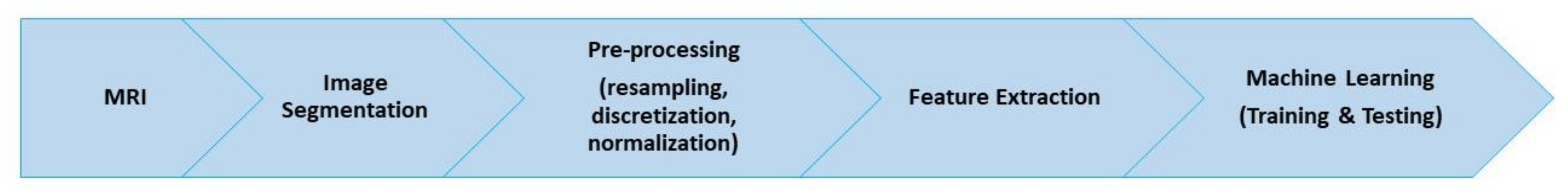
2. Materials and Methods
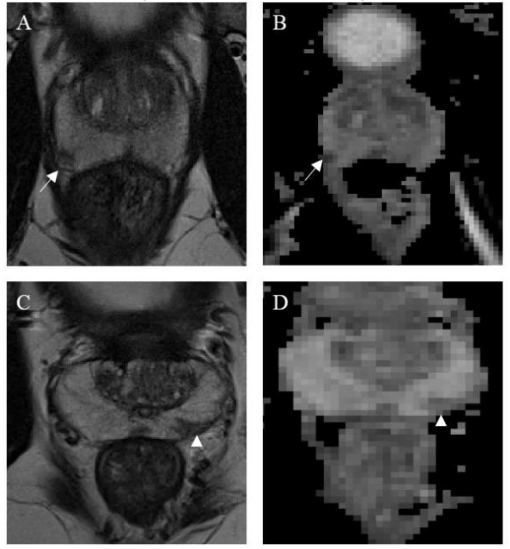
2.1. Dataset
2.2. Radiomics Features Extraction
2.3. Statistical Analysis
2.4. Machine Learning
3. Results
3.1. Statistical Analysis
3.2. Machine Learning Analysis
4. Discussion and Conclusions
Author Contributions
Funding
Institutional Review Board Statement
Informed Consent Statement
Data Availability Statement
Conflicts of Interest
Appendix A
- t2_log-sigma-3-0-mm-3D_glcm_Contrast
- t2_log-sigma-3-0-mm-3D_ngtdm_Busyness
- t2_log-sigma-4-0-mm-3D_firstorder_10Percentile
- t2_log-sigma-4-0-mm-3D_firstorder_90Percentile
- t2_log-sigma-4-0-mm-3D_firstorder_InterquartileRange
- t2_log-sigma-4-0-mm-3D_glcm_Idm
- t2_log-sigma-4-0-mm-3D_glcm_InverseVariance
- t2_log-sigma-5-0-mm-3D_firstorder_Minimum
- t2_log-sigma-5-0-mm-3D_glcm_Contrast
- t2_log-sigma-5-0-mm-3D_glszm_LargeAreaEmphasis
- t2_log-sigma-5-0-mm-3D_gldm_LargeDependenceHighGrayLevelEmphasis
- t2_wavelet-LLH_glcm_JointEnergy
- t2_wavelet-LHL_firstorder_90Percentile
- t2_wavelet-LHH_glcm_JointEnergy
- t2_wavelet-HLL_glrlm_LongRunEmphasis
- t2_wavelet-HHL_firstorder_Variance
- t2_wavelet-HHL_glszm_LargeAreaLowGrayLevelEmphasis
- t2_wavelet-HHL_ngtdm_Busyness
- t2_wavelet-LLL_firstorder_Energy
- adc_original_firstorder_10Percentile
- adc_original_glrlm_LongRunEmphasis
- adc_original_glszm_LargeAreaEmphasis
- adc_log-sigma-1-0-mm-3D_glcm_Contrast
- adc_log-sigma-1-0-mm-3D_glcm_Idm
- adc_log-sigma-3-0-mm-3D_firstorder_90Percentile
- adc_log-sigma-3-0-mm-3D_glrlm_LongRunEmphasis
- adc_log-sigma-3-0-mm-3D_glszm_GrayLevelNonUniformity
- adc_log-sigma-4-0-mm-3D_glcm_InverseVariance
- adc_log-sigma-4-0-mm-3D_glszm_LargeAreaHighGrayLevelEmphasis
- adc_log-sigma-5-0-mm-3D_glrlm_RunPercentage
- adc_log-sigma-5-0-mm-3D_glszm_ZoneVariance
- adc_wavelet-LHL_firstorder_Kurtosis
- adc_wavelet-HLL_firstorder_90Percentile
- adc_wavelet-HLL_glcm_Imc2
- adc_wavelet-HLL_glcm_Idm
- adc_wavelet-HLL_glrlm_RunVariance
- adc_wavelet-HHL_glcm_Contrast
- adc_wavelet-HHL_glszm_LargeAreaEmphasis
- adc_wavelet-LLL_glcm_Imc2
References
- Siegel, R.L.; Miller, K.D.; Fuchs, H.E.; Jemal, A. Cancer statistics. CA Cancer J. Clin. 2021, 71, 7–33. [Google Scholar] [CrossRef]
- Matoso, A.; Epstein, J.I. Defining clinically significant prostate cancer on the basis of pathological findings. Histopathology 2019, 74, 135–145. [Google Scholar] [CrossRef] [Green Version]
- Mottet, N.; Van den Bergh, R.C.N.; Briers, E.; Van den Broeck, T.; Cumberbatch, M.G.; De Santis, M.; Fanti, S.; Fossati, N.; Gandaglia, G.; Gillessen, S.; et al. EAU-EANM-ESTRO-ESUR-SIOG Guidelines on Prostate Cancer-2020 Update. Part 1: Screening, Diagnosis, and Local Treatment with Curative Intent. Eur. Urol. 2021, 79, 243–262. [Google Scholar] [CrossRef] [PubMed]
- Gupta, R.T.; Mehta, K.A.; Turkbey, B.; Verma, S. PI-RADS: Past, present, and future. J. Magn. Reson. Imaging 2020, 52, 33–53. [Google Scholar] [CrossRef] [PubMed]
- Del Monte, M.; Leonardo, C.; Salvo, V.; Grompone, M.D.; Pecoraro, M.; Stanzione, A.; Campa, R.; Vullo, F.; Sciarra, A.; Catalano, V.; et al. MRI/US fusion-guided biopsy: Performing exclusively targeted biopsies for the early detection of prostate cancer. Radiol. Med. 2018, 123, 227–234. [Google Scholar] [CrossRef] [PubMed]
- Wei, C.G.; Zhang, Y.Y.; Pan, P.; Chen, T.; Yu, H.C.; Dai, G.C.; Tu, J.; Yang, S.; Zhao, W.L.; Shen, J.K. Diagnostic accuracy and interobserver agreement of PI-RADS version 2 and version 2.1 for the detection of transition zone prostate cancers. Am. J. Roentgenol. 2021, 216, 1247–1256. [Google Scholar] [CrossRef]
- Sosnowski, R.; Zagrodzka, M.; Borkowski, T. The limitations of multiparametric magnetic resonance imaging also must be borne in mind. Cent. Eur. J. Urol. 2016, 69, 22–23. [Google Scholar] [CrossRef] [Green Version]
- Stanzione, A.; Ricciardi, C.; Cuocolo, R.; Romeo, V.; Petrone, J.; Sarnataro, M.; Mainenti, P.P.; Improta, G.; De Rosa, F.; Insabato, L.; et al. MRI Radiomics for the Prediction of Fuhrman Grade in Clear Cell Renal Cell Carcinoma: A Machine Learning Exploratory Study. J. Digit. Imaging 2020, 33, 879–887. [Google Scholar] [CrossRef]
- Carlo, R.; Renato, C.; Giuseppe, C.; Lorenzo, U.; Giovanni, I.; Domenico, S.; Valeria, R.; Elia, G.; Maria, C.L.; Mario, C. Distinguishing Functional from Non-functional Pituitary Macroadenomas with a Machine Learning Analysis. In Proceedings of the XV Mediterranean Conference on Medical and Biological Engineering and Computing—MEDICON 2019, IFMBE Proceedings, Coimbra, Portugal, 26–28 September 2019; Henriques, J., Neves, N., de Carvalho, P., Eds.; Springer: Cham, Switzerland, 2020; Volume 76. [Google Scholar] [CrossRef]
- Romeo, V.; Cuocolo, R.; Ricciardi, C.; Ugga, L.; Cocozza, S.; Verde, F.; Stanzione, A.; Napolitano, V.; Russo, D.; Improta, G.; et al. Prediction of tumor grade and nodal status in oropharyngeal and oral cavity squamous-cell carcinoma using a radiomic approach. Anticancer. Res. 2020, 40, 271–280. [Google Scholar] [CrossRef]
- Chaddad, A.; Kucharczyk, M.J.; Cheddad, A.; Clarke, S.E.; Hassan, L.; Ding, S.; Rathore, S.; Zhang, M.; Katib, Y.; Bahoric, B.; et al. Magnetic resonance imaging based radiomic models of prostate cancer: A narrative review. Cancers 2021, 13, 552. [Google Scholar] [CrossRef]
- Stanzione, A.; Gambardella, M.; Cuocolo, R.; Ponsiglione, A.; Romeo, V.; Imbriaco, M. Prostate MRI radiomics: A systematic review and radiomic quality score assessment. Eur. J. Radiol. 2020, 129, 109095. [Google Scholar] [CrossRef]
- Cuocolo, R.; Cipullo, M.B.; Stanzione, A.; Romeo, V.; Green, R.; Cantoni, V.; Ponsiglione, A.; Ugga, L.; Imbriaco, M. Machine learning for the identification of clinically significant prostate cancer on MRI: A meta-analysis. Eur. Radiol. 2020, 30, 6877–6887. [Google Scholar] [CrossRef] [PubMed]
- Cutaia, G.; La Tona, G.; Comelli, A.; Vernuccio, F.; Agnello, F.; Gagliardo, C.; Salvaggio, L.; Quartuccio, N.; Sturiale, L.; Stefano, A.; et al. Radiomics and Prostate MRI: Current Role and Future Applications. J. Imaging 2021, 7, 34. [Google Scholar] [CrossRef] [PubMed]
- Spadarella, G.; Calareso, G.; Garanzini, E.; Ugga, L.; Cuocolo, A.; Cuocolo, R. MRI based radiomics in nasopharyngeal cancer: Systematic review and perspectives using radiomic quality score (RQS) assessment. Eur. J. Radiol. 2021, 140, 109744. [Google Scholar] [CrossRef] [PubMed]
- Cuocolo, R.; Stanzione, A.; Castaldo, A.; De Lucia, D.R.; Imbriaco, M. Quality control and whole-gland, zonal and lesion annotations for the PROSTATEx challenge public dataset. Eur. J. Radiol. 2021, 138, 109647. [Google Scholar] [CrossRef]
- Litjens, G.; Debats, O.; Barentsz, J.; Karssemeijer, N.; Huisman, H. Computer-aided detection of prostate cancer in MRI. IEEE Trans. Med Imaging 2014, 33, 1083–1092. [Google Scholar] [CrossRef] [PubMed]
- Steiger, P.; Thoeny, H.C. Prostate MRI based on PI-RADS version 2: How we review and report. Cancer Imaging 2016, 16, 9. [Google Scholar] [CrossRef] [PubMed] [Green Version]
- Litjens, G.; Debats, O.; van de Ven, W.; Karssemeijer, N.; Huisman, H. A pattern recognition approach to zonal segmentation of the prostate on MRI. In Proceedings of the International Conference on Medical Image Computing and Computer-Assisted Intervention, Nice, France, 1–5 October 2012; Springer: Berlin/Heidelberg, Germany, 2012; pp. 413–420. [Google Scholar]
- Stanzione, A.; Cuocolo, R.; Del Grosso, R.; Nardiello, A.; Romeo, V.; Travaglino, A.; Raffone, A.; Bifulco, G.; Zullo, F.; Insabato, L.; et al. Deep myometrial infiltration of endometrial cancer on MRI: A radiomics-powered machine learning pilot study. Acad. Radiol. 2021, 28, 737–744. [Google Scholar] [CrossRef]
- Van Griethuysen, J.J.; Fedorov, A.; Parmar, C.; Hosny, A.; Aucoin, N.; Narayan, V.; Beets-Tan, R.G.; Fillion-Robin, J.C.; Pieper, S.; Aerts, H.J. Computational radiomics system to decode the radiographic phenotype. Cancer Res. 2017, 77, e104–e107. [Google Scholar] [CrossRef] [Green Version]
- Cuocolo, R.; Stanzione, A.; Faletti, R.; Gatti, M.; Calleris, G.; Fornari, A.; Gentile, F.; Motta, A.; Dell’Aversana, S.; Creta, M.; et al. MRI index lesion radiomics and machine learning for detection of extraprostatic extension of disease: A multicenter study. Eur. Radiol. 2021, 31, 7575–7583. [Google Scholar] [CrossRef]
- Klein, S.; Van Der Heide, U.A.; Lips, I.M.; Van Vulpen, M.; Staring, M.; Pluim, J.P. Automatic segmentation of the prostate in 3D MR images by atlas matching using localized mutual information. Med. Phys. 2008, 35, 1407–1417. [Google Scholar] [CrossRef]
- Ali, J.; Khan, R.; Ahmad, N.; Maqsood, I. Random forests and decision trees. Int. J. Comput. Sci. Issues (IJCSI) 2012, 9, 272. [Google Scholar]
- Quinlan, J.R. C4. 5: Programs for Machine Learning; Elsevier: Amsterdam, The Netherlands, 1994. [Google Scholar]
- Breiman, L. Random forests. Mach. Learn. 2001, 45, 5–32. [Google Scholar] [CrossRef] [Green Version]
- Si, S.; Zhang, H.; Keerthi, S.S.; Mahajan, D.; Dhillon, I.S.; Hsieh, C.J. Gradient boosted decision trees for high dimensional sparse output. In Proceedings of the 34th International Conference on Machine Learning, PMLR, Sydney, Australia, 6–11 August 2017; pp. 3182–3190. [Google Scholar]
- Freund, Y.; Schapire, R.E. A decision-theoretic generalization of on-line learning and an application to boosting. J. Comput. Syst. Sci. 1997, 55, 119–139. [Google Scholar] [CrossRef] [Green Version]
- Hong, H.; Liu, J.; Bui, D.T.; Pradhan, B.; Acharya, T.D.; Pham, B.T.; Zhu, A.X.; Chen, W.; Ahmad, B.B. Landslide susceptibility mapping using J48 Decision Tree with AdaBoost, Bagging and Rotation Forest ensembles in the Guangchang area (China). Catena 2018, 163, 399–413. [Google Scholar] [CrossRef]
- Rish, I. An empirical study of the naive Bayes classifier. In IJCAI 2001 Workshop on Empirical Methods in Artificial Intelligence; IBM: New York, NY, USA, 2001; Volume 3, pp. 41–46. [Google Scholar]
- Langley, P.; Iba, W.; Thompson, K. An analysis of Bayesian classifiers. In Proceedings of the Tenth National Conference on Artificial Intelligence, AAAI’92, San Jose, CA, USA, 12–16 July 1992; AAAI: Menlo Park, CA, USA, 1992; Volume 90, pp. 223–228. [Google Scholar]
- Mitchell, T.M. Machine Learning; McGraw-Hill Education: New York, NY, USA, 1997. [Google Scholar]
- Chomboon, K.; Chujai, P.; Teerarassamee, P.; Kerdprasop, K.; Kerdprasop, N. An empirical study of distance metrics for k-nearest neighbor algorithm. In Proceedings of the 3rd International Conference on Industrial Application Engineering, Kitakyushu, Japan, 28–31 March 2015; pp. 280–285. [Google Scholar]
- Anguita, D.; Ghelardoni, L.; Ghio, A.; Oneto, L.; Ridella, S. The ‘K’ in K-fold Cross Validation. In Proceedings of the European Symposium on Artificial Neural Networks, Computational Intelligence and Machine Learning (ESANN), Bruges, Belgium, 25–27 April 2012; pp. 441–446. [Google Scholar]
- Yadav, S.; Shukla, S. Analysis of k-fold cross-validation over hold-out validation on colossal datasets for quality classification. In Proceedings of the 2016 IEEE 6th International Conference on Advanced Computing (IACC), Bhimavaram, India, 27–28 February 2016; pp. 78–83. [Google Scholar]
- Kostrzewa, D.; Brzeski, R. The data dimensionality reduction in the classification process through greedy backward feature elimination. In Proceedings of the International Conference on Man–Machine Interactions, Kraków, Poland, 3–6 October 2017; Springer: Cham, Switzerland, 2017; pp. 397–407. [Google Scholar]
- Hossin, M.; Sulaiman, M.N. A review on evaluation metrics for data classification evaluations. Int. J. Data Min. Knowl. Manag. Process. 2015, 5, 1–11. [Google Scholar]
- Scrutinio, D.; Ricciardi, C.; Donisi, L.; Losavio, E.; Battista, P.; Guida, P.; Cesarelli, M.; Pagano, G.; D’Addio, G. Machine learning to predict mortality after rehabilitation among patients with severe stroke. Sci. Rep. 2020, 10, 20127. [Google Scholar] [CrossRef]
- O’Hagan, S.; Kell, D.B. Software review: The KNIME workflow environment and its applications in Genetic Programming and machine learning. Genet. Program. Evolvable Mach. 2015, 16, 387–391. [Google Scholar] [CrossRef] [Green Version]
- Donisi, L.; Cesarelli, G.; Coccia, A.; Panigazzi, M.; Capodaglio, E.M.; D’Addio, G. Work-Related Risk Assessment According to the Revised NIOSH Lifting Equation: A Preliminary Study Using a Wearable Inertial Sensor and Machine Learning. Sensors 2021, 21, 2593. [Google Scholar] [CrossRef] [PubMed]
- Crawford, E.D.; Grubb, R., 3rd; Black, A.; Andriole, G.L., Jr.; Chen, M.H.; Izmirlian, G.; Berg, C.D.; D’Amico, A.V. Comorbidity and mortality results from a randomized prostate cancer screening trial. J. Clin. Oncol. Off. J. Am. Soc. Clin. Oncol. 2011, 29, 355–361. [Google Scholar] [CrossRef] [PubMed]
- Tosoian, J.J.; Carter, H.B.; Lepor, A.; Loeb, S. Active surveillance for prostate cancer: Current evidence and contemporary state of practice. Nat. Rev. Urol. 2016, 13, 205–215. [Google Scholar] [CrossRef] [Green Version]
- Edmund, L.; Rotker, K.L.; Lakis, N.S.; Brito, J.M., III; Lepe, M.; Lombardo, K.A.; Renzulli, J.F., II; Matoso, A. Upgrading and upstaging at radical prostatectomy in the post-prostate-specific antigen screening era: An effect of delayed diagnosis or a shift in patient selection? Hum. Pathol. 2017, 59, 87–93. [Google Scholar] [CrossRef]
- Abraham, B.; Nair, M.S. Computer-aided grading of prostate cancer from MRI images using convolutional neural networks. J. Intell. Fuzzy Syst. 2019, 36, 2015–2024. [Google Scholar] [CrossRef]
- Le, M.H.; Chen, J.; Wang, L.; Wang, Z.; Liu, W.; Cheng, K.T.T.; Yang, X. Automated diagnosis of prostate cancer in multi-parametric MRI based on multimodal convolutional neural networks. Phys. Med. Biol. 2017, 62, 6497–6514. [Google Scholar] [CrossRef]
- Sobecki, P.; Życka-Malesa, D.; Mykhalevych, I.; Sklinda, K.; Przelaskowski, A. MRI imaging texture features in prostate lesions classification. In EMBEC & NBC 2017. EMBEC 2017, NBC 2017, IFMBE Proceedings; Eskola, H., Väisänen, O., Viik, J., Hyttinen, J., Eds.; Springer: Singapore, 2018; Volume 65, pp. 827–830. [Google Scholar]
- Zhong, X.; Cao, R.; Shakeri, S.; Scalzo, F.; Lee, Y.; Enzmann, D.R.; Wu, H.H.; Raman, S.S.; Sung, K. Deep transfer learning- based prostate cancer classification using 3 Tesla multi-parametric MRI. Abdom. Radiol. 2019, 44, 2030–2039. [Google Scholar] [CrossRef]
- Chaddad, A.; Niazi, T.; Probst, S.; Bladou, F.; Anidjar, M.; Bahoric, B. Predicting Gleason score of prostate cancer patients using radiomic analysis. Front. Oncol. 2018, 8, 630. [Google Scholar] [CrossRef] [PubMed] [Green Version]
- Chen, T.; Li, M.; Gu, Y.; Zhang, Y.; Yang, S.; Wei, C.; Wu, J.; Li, X.; Zhao, W.; Shen, J. Prostate cancer differentiation and aggressiveness: Assessment with a radiomic-based model vs. PI-RADS v2. J. Magn. Reson. Imaging 2019, 49, 875–884. [Google Scholar] [CrossRef] [PubMed] [Green Version]
- Fehr, D.; Veeraraghavan, H.; Wibmer, A.; Gondo, T.; Matsumoto, K.; Vargas, H.A.; Sala, E.; Hricak, H.; Deasy, J.O. Automatic classification of prostate cancer Gleason scores from multiparametric magnetic resonance images. Proc. Natl. Acad. Sci. USA 2015, 112, E6265–E6273. [Google Scholar] [CrossRef] [Green Version]
- Bonekamp, D.; Kohl, S.; Wiesenfarth, M.; Schelb, P.; Radtke, J.P.; Götz, M.; Kickingereder, P.; Yaqubi, K.; Hitthaler, B.; Gählert, N.; et al. Radiomic machine learning for characterization of prostate lesions with MRI: Comparison to ADC values. Radiology 2018, 289, 128–137. [Google Scholar] [CrossRef] [PubMed]
- Peerlings, J.; Woodruff, H.C.; Winfield, J.M.; Ibrahim, A.; Van Beers, B.E.; Heerschap, A.; Jackson, A.; Wildberger, J.E.; Mottaghy, F.M.; DeSouza, N.M.; et al. Stability of radiomics features in apparent diffusion coefficient maps from a multi-centre test-retest trial. Sci. Rep. 2019, 9, 4800. [Google Scholar] [CrossRef] [Green Version]
- Rundo, L.; Militello, C.; Russo, G.; Garufi, A.; Vitabile, S.; Gilardi, M.C.; Mauri, G. Automated prostate gland segmentation based on an unsupervised fuzzy C-means clustering technique using multispectral T1w and T2w MR imaging. Information 2017, 8, 49. [Google Scholar] [CrossRef] [Green Version]
- Wang, Z.; Liu, C.; Cheng, D.; Wang, L.; Yang, X.; Cheng, K.T. Automated detection of clinically significant prostate cancer in mp-MRI images based on an end-to-end deep neural network. IEEE Trans. Med Imaging 2018, 37, 1127–1139. [Google Scholar] [CrossRef]
- Antonelli, M.; Johnston, E.W.; Dikaios, N.; Cheung, K.K.; Sidhu, H.S.; Appayya, M.B.; Giganti, F.; Simmons, L.A.; Freeman, A.; Allen, C.; et al. Machine learning classifiers can predict Gleason pattern 4 prostate cancer with greater accuracy than experienced radiologists. Eur. Radiol. 2019, 29, 4754–4764. [Google Scholar] [CrossRef] [Green Version]
- Dikaios, N.; Alkalbani, J.; Abd-Alazeez, M.; Sidhu, H.S.; Kirkham, A.; Ahmed, H.U.; Emberton, M.; Freeman, A.; Halligan, S.; Taylor, S.; et al. Zone-specific logistic regression models improve classification of prostate cancer on multi-parametric MRI. Eur. Radiol. 2015, 25, 2727–2737. [Google Scholar] [CrossRef]
- Clark, K.; Vendt, B.; Smith, K.; Freymann, J.; Kirby, J.; Koppel, P.; Moore, S.; Phillips, S.; Maffitt, D.; Pringle, M.; et al. The cancer imaging archive (TCIA): Maintaining and operating a public information repository. J. Digit. Imaging 2013, 26, 1045–1057. [Google Scholar] [CrossRef] [PubMed] [Green Version]
- Lapa, P.; Castelli, M.; Gonçalves, I.; Sala, E.; Rundo, L. A Hybrid End-to-End Approach Integrating Conditional Random Fields into CNNs for Prostate Cancer Detection on MRI. Appl. Sci. 2020, 10, 338. [Google Scholar] [CrossRef] [Green Version]
- Kang, H.C.; Jo, N.; Bamashmos, A.S.; Ahmed, M.; Sun, J.; Ward, J.F.; Choi, H. Accuracy of Prostate Magnetic Resonance Imaging: Reader Experience Matters. Eur. Urol. Open Sci. 2021, 27, 53–60. [Google Scholar] [CrossRef] [PubMed]
- Cuocolo, R.; Verde, F.; Ponsiglione, A.; Romeo, V.; Petretta, M.; Imbriaco, M.; Stanzione, A. Clinically significant prostate cancer detection with biparametric MRI: A systematic review and meta-analysis. Am. J. Roentgenol. 2021, 216, 608–621. [Google Scholar] [CrossRef] [PubMed]
- Pasquini, L.; Napolitano, A.; Visconti, E.; Longo, D.; Romano, A.; Tomà, P.; Espagnet, M.C.R. Gadolinium-based contrast agent-related toxicities. CNS Drugs 2018, 32, 229–240. [Google Scholar] [CrossRef]
- Wallström, J.; Geterud, K.; Kohestani, K.; Maier, S.E.; Månsson, M.; Pihl, C.G.; Socratous, A.; Godtman, R.A.; Hellström, M.; Hugosson, J. Bi- or multiparametric MRI in a sequential screening program for prostate cancer with PSA followed by MRI? Results from the Göteborg prostate cancer screening 2 trial. Eur. Radiol. 2021, 1–11. [Google Scholar] [CrossRef]


| Variable | Class | Mean | ± | std. dev. | t-Test p-Value |
|---|---|---|---|---|---|
| t2_original_shape_MeshVolume | 0 | 0.11 | ± | 0.13 | 0.003 ** |
| 1 | 0.18 | ± | 0.19 | ||
| t2_original_firstorder_10Percentile | 0 | 0.47 | ± | 0.20 | 0.002 ** |
| 1 | 0.40 | ± | 0.15 | ||
| t2_original_glcm_Imc2 | 0 | 0.65 | ± | 0.26 | 0.007 ** |
| 1 | 0.56 | ± | 0.26 | ||
| t2_original_glcm_Idm | 0 | 0.59 | ± | 0.16 | 0.098 |
| 1 | 0.62 | ± | 0.15 | ||
| t2_logsigma10mm3D_firstorder_90Percentile | 0 | 0.24 | ± | 0.15 | 0.119 |
| 1 | 0.21 | ± | 0.13 | ||
| t2_logsigma10mm3D_ngtdm_Busyness | 0 | 0.15 | ± | 0.15 | 0.042 * |
| 1 | 0.20 | ± | 0.19 | ||
| t2_logsigma10mm3D_gldm_DependenceVariance | 0 | 0.37 | ± | 0.21 | 0.001 *** |
| 1 | 0.46 | ± | 0.21 | ||
| t2_logsigma20mm3D_firstorder_90Percentile | 0 | 0.44 | ± | 0.19 | 0.874 |
| 1 | 0.44 | ± | 0.15 | ||
| t2_logsigma20mm3D_glcm_DifferenceVariance | 0 | 0.19 | ± | 0.16 | 0.506 |
| 1 | 0.17 | ± | 0.15 | ||
| t2_logsigma20mm3D_glszm_LargeAreaLowGrayLevelEmphasis | 0 | 4.76 | ± | 1.17 | 0.345 |
| 1 | 6.16 | ± | 9.36 | ||
| t2_logsigma30mm3D_glcm_Contrast | 0 | 0.15 | ± | 0.13 | 0.112 |
| 1 | 0.12 | ± | 0.11 | ||
| t2_logsigma30mm3D_glrlm_LongRunEmphasis | 0 | 0.25 | ± | 0.17 | 0.015 * |
| 1 | 0.31 | ± | 0.19 | ||
| t2_logsigma30mm3D_ngtdm_Busyness | 0 | 0.15 | ± | 0.15 | 0.181 |
| 1 | 0.17 | ± | 0.13 | ||
| t2_logsigma40mm3D_firstorder_10Percentile | 0 | 0.63 | ± | 0.17 | 0.072 |
| 1 | 0.66 | ± | 0.12 | ||
| t2_logsigma40mm3D_firstorder_90Percentile | 0 | 0.44 | ± | 0.17 | 0.033 * |
| 1 | 0.49 | ± | 0.14 | ||
| t2_logsigma40mm3D_firstorder_InterquartileRange | 0 | 0.38 | ± | 0.17 | 0.571 |
| 1 | 0.39 | ± | 0.19 | ||
| t2_logsigma40mm3D_glcm_Idm | 0 | 0.50 | ± | 0.17 | 0.054 |
| 1 | 0.54 | ± | 0.16 | ||
| t2_logsigma40mm3D_glcm_InverseVariance | 0 | 0.85 | ± | 0.11 | 0.325 |
| 1 | 0.86 | ± | 0.08 | ||
| t2_logsigma40mm3D_glszm_SizeZoneNonUniformity | 0 | 0.07 | ± | 0.10 | 0.064 |
| 1 | 0.11 | ± | 0.14 | ||
| t2_logsigma50mm3D_firstorder_Minimum | 0 | 0.58 | ± | 0.17 | 0.708 |
| 1 | 0.57 | ± | 0.14 | ||
| t2_logsigma50mm3D_firstorder_Variance | 0 | 0.17 | ± | 0.15 | 0.026 * |
| 1 | 0.22 | ± | 0.17 | ||
| t2_logsigma50mm3D_glcm_Autocorrelation | 0 | 0.16 | ± | 0.15 | 0.006 ** |
| 1 | 0.22 | ± | 0.16 | ||
| t2_logsigma50mm3D_glcm_Contrast | 0 | 0.11 | ± | 0.11 | 0.465 |
| 1 | 0.10 | ± | 0.82 | ||
| t2_logsigma50mm3D_glrlm_LongRunEmphasis | 0 | 0.26 | ± | 0.16 | 0.413 |
| 1 | 0.28 | ± | 0.18 | ||
| t2_logsigma50mm3D_glszm_LargeAreaEmphasis | 0 | 5.40 | ± | 1.16 | 0.172 |
| 1 | 7.50 | ± | 1.13 | ||
| t2_logsigma50mm3D_gldm_LargeDependenceHighGrayLevelEmphasis | 0 | 0.09 | ± | 0.10 | 0.003 ** |
| 1 | 0.13 | ± | 0.11 | ||
| t2_waveletLLH_glcm_JointEnergy | 0 | 0.28 | ± | 0.19 | 0.927 |
| 1 | 0.28 | ± | 0.15 | ||
| t2_waveletLHL_firstorder_90Percentile | 0 | 0.21 | ± | 0.15 | 0.213 |
| 1 | 0.19 | ± | 0.12 | ||
| t2_waveletLHH_glcm_JointEnergy | 0 | 0.45 | ± | 0.21 | 0.305 |
| 1 | 0.47 | ± | 0.17 | ||
| t2_waveletHLL_glrlm_LongRunEmphasis | 0 | 0.36 | ± | 0.16 | 0.217 |
| 1 | 0.38 | ± | 0.17 | ||
| t2_waveletHLL_ngtdm_Busyness | 0 | 0.14 | ± | 0.14 | 0.059 |
| 1 | 0.17 | ± | 0.17 | ||
| t2_waveletHHL_firstorder_Variance | 0 | 0.24 | ± | 0.14 | 0.244 |
| 1 | 0.22 | ± | 0.11 | ||
| t2_waveletHHL_glszm_LargeAreaLowGrayLevelEmphasis | 0 | 0.40 | ± | 0.08 | 0.386 |
| 1 | 0.06 | ± | 0.15 | ||
| t2_waveletHHL_ngtdm_Busyness | 0 | 0.17 | ± | 0.17 | 0.047 * |
| 1 | 0.22 | ± | 0.19 | ||
| t2_waveletLLL_firstorder_Energy | 0 | 0.10 | ± | 0.14 | 0.131 |
| 1 | 0.13 | ± | 0.15 | ||
| adc_original_firstorder_10Percentile | 0 | 0.58 | ± | 0.16 | 0.001 *** |
| 1 | 0.47 | ± | 0.18 | ||
| adc_original_glrlm_LongRunEmphasis | 0 | 0.31 | ± | 0.18 | 0.612 |
| 1 | 0.32 | ± | 0.17 | ||
| adc_logsigma10mm3D_glcm_Contrast | 0 | 0.10 | ± | 0.11 | 0.718 |
| 1 | 0.09 | ± | 0.09 | ||
| adc_logsigma10mm3D_glcm_Idm | 0 | 0.54 | ± | 0.21 | 0.265 |
| 1 | 0.57 | ± | 0.19 | ||
| adc_logsigma10mm3D_ngtdm_Strength | 0 | 0.11 | ± | 0.15 | 0.070 |
| 1 | 0.09 | ± | 0.09 | ||
| adc_logsigma30mm3D_firstorder_90Percentile | 0 | 0.11 | ± | 0.14 | 0.001 *** |
| 1 | 0.09 | ± | 0.09 | ||
| adc_logsigma30mm3D_glcm_DifferenceAverage | 0 | 0.35 | ± | 0.19 | 0.163 |
| 1 | 0.38 | ± | 0.16 | ||
| adc_logsigma30mm3D_glrlm_LongRunEmphasis | 0 | 0.26 | ± | 0.16 | 0.140 |
| 1 | 0.23 | ± | 0.12 | ||
| adc_logsigma30mm3D_glszm_GrayLevelNonUniformity | 0 | 0.16 | ± | 0.13 | 0.001 *** |
| 1 | 0.25 | ± | 0.21 | ||
| adc_logsigma40mm3D_glcm_InverseVariance | 0 | 0.66 | ± | 0.16 | 0.694 |
| 1 | 0.65 | ± | 0.16 | ||
| adc_logsigma40mm3D_glszm_LargeAreaHighGrayLevelEmphasis | 0 | 4.28 × 10² | ± | 1.22 × 10² | 0.472 |
| 1 | 5.39 × 10² | ± | 9.64 × 10² | ||
| adc_logsigma50mm3D_firstorder_10Percentile | 0 | 0.50 | ± | 0.18 | 0.100 |
| 1 | 0.54 | ± | 0.19 | ||
| adc_logsigma50mm3D_glrlm_RunPercentage | 0 | 0.58 | ± | 0.15 | 0.051 |
| 1 | 0.62 | ± | 0.12 | ||
| adc_logsigma50mm3D_glszm_ZoneVariance | 0 | 6.50 × 10² | ± | 1.39 × 101 | 0.720 |
| 1 | 5.99 × 10² | ± | 8.49 × 10² | ||
| adc_waveletLLH_glcm_JointEnergy | 0 | 0.27 | ± | 0.16 | 0.572 |
| 1 | 0.29 | ± | 0.18 | ||
| adc_waveletLLH_glrlm_LongRunEmphasis | 0 | 0.19 | ± | 0.12 | 0.015 * |
| 1 | 0.24 | ± | 0.16 | ||
| adc_waveletLHL_firstorder_90Percentile | 0 | 0.36 | ± | 0.14 | 0.926 |
| 1 | 0.36 | ± | 0.13 | ||
| adc_waveletLHL_firstorder_Kurtosis | 0 | 0.10 | ± | 0.10 | 0.004 ** |
| 1 | 0.15 | ± | 0.14 | ||
| adc_waveletHLL_firstorder_90Percentile | 0 | 0.22 | ± | 0.12 | 0.060 |
| 1 | 0.25 | ± | 0.12 | ||
| adc_waveletHLL_glcm_Imc2 | 0 | 0.46 | ± | 0.23 | 0.984 |
| 1 | 0.46 | ± | 0.20 | ||
| adc_waveletHLL_glcm_Idm | 0 | 0.53 | ± | 0.16 | 0.743 |
| 1 | 0.53 | ± | 0.14 | ||
| adc_waveletHLL_glrlm_RunVariance | 0 | 0.28 | ± | 0.15 | 0.05 * |
| 1 | 0.32 | ± | 0.18 | ||
| adc_waveletHHL_glcm_Contrast | 0 | 0.07 | ± | 0.12 | 0.834 |
| 1 | 0.08 | ± | 0.10 | ||
| adc_waveletHHL_glszm_LargeAreaEmphasis | 0 | 4.70 × 10² | ± | 8.20 × 10² | 0.064 |
| 1 | 8.26 × 10² | ± | 1.58 × 101 | ||
| adc_waveletLLL_glcm_Imc2 | 0 | 0.88 | ± | 0.17 | 0.477 |
| 1 | 0.89 | ± | 0.12 |
| Algorithms | Accuracy | Accuracy Max | Sensitivity | Specificity | AUCROC |
|---|---|---|---|---|---|
| J48 | 74.2 | 83.3 | 35.5 | 87.4 | 0.567 |
| ADA-B | 74.6 | 86.7 | 42.1 | 85.7 | 0.720 |
| RF | 77.9 | 83.3 | 48.7 | 87.9 | 0.713 |
| GBT | 74.9 | 86.2 | 34.2 | 88.8 | 0.682 |
| NB | 68.9 | 80.0 | 56.6 | 73.1 | 0.650 |
| KNN | 73.2 | 76.7 | 18.4 | 91.9 | 0.643 |
| Algorithms | Number of Features | Accuracy | Accuracy Max | Sensitivity | Specificity | AUCROC |
|---|---|---|---|---|---|---|
| J48 | 16 | 82.2 | 100 | 56.5 | 91.0 | 0.635 |
| ADA-B | 14 | 81.1 | 88.9 | 52.2 | 91.0 | 0.708 |
| RF | 39 | 82.2 | 88.9 | 39.1 | 97.0 | 0.730 |
| GBT | 50 | 76.7 | 100 | 43.5 | 88.1 | 0.774 |
| NB | 15 | 70.0 | 88.9 | 21.7 | 86.6 | 0.546 |
| KNN | 25 | 74.4 | 88.9 | 30.4 | 89.6 | 0.676 |
Publisher’s Note: MDPI stays neutral with regard to jurisdictional claims in published maps and institutional affiliations. |
© 2021 by the authors. Licensee MDPI, Basel, Switzerland. This article is an open access article distributed under the terms and conditions of the Creative Commons Attribution (CC BY) license (https://creativecommons.org/licenses/by/4.0/).
Share and Cite
Donisi, L.; Cesarelli, G.; Castaldo, A.; De Lucia, D.R.; Nessuno, F.; Spadarella, G.; Ricciardi, C. A Combined Radiomics and Machine Learning Approach to Distinguish Clinically Significant Prostate Lesions on a Publicly Available MRI Dataset. J. Imaging 2021, 7, 215. https://0-doi-org.brum.beds.ac.uk/10.3390/jimaging7100215
Donisi L, Cesarelli G, Castaldo A, De Lucia DR, Nessuno F, Spadarella G, Ricciardi C. A Combined Radiomics and Machine Learning Approach to Distinguish Clinically Significant Prostate Lesions on a Publicly Available MRI Dataset. Journal of Imaging. 2021; 7(10):215. https://0-doi-org.brum.beds.ac.uk/10.3390/jimaging7100215
Chicago/Turabian StyleDonisi, Leandro, Giuseppe Cesarelli, Anna Castaldo, Davide Raffaele De Lucia, Francesca Nessuno, Gaia Spadarella, and Carlo Ricciardi. 2021. "A Combined Radiomics and Machine Learning Approach to Distinguish Clinically Significant Prostate Lesions on a Publicly Available MRI Dataset" Journal of Imaging 7, no. 10: 215. https://0-doi-org.brum.beds.ac.uk/10.3390/jimaging7100215