
Enhanced Region Growing for Brain Tumor MR Image Segmentation

 , ,
, ,
Abstract
:1. Introduction
- Benign brain tumors are those that grow slowly and do not metastasize or spread to other body organs and often can be removed and hence are less destructive or curable. They can still cause problems since they can grow big and press on sensitive areas of the brain (the so-called mass effect). Depending on their location, they can be life-threatening.
- Malignant brain tumors are those with cancerous cells. The rate of growth is fast ranging from months to a few years. Unlike other malignancies, malignant brain tumors rarely spread to other body parts due to the tight junction in the brain and spinal cord.
Brain Tumor Imaging Technologies
- T1-weighted: by measuring the time required for the magnetic vector to return to its resting state(T1-relaxation time)
- T2-weighted: by measuring the time required for the axial spin to return to its resting state (T2-relaxation time).
- Fluid-attenuated inversion recovery(T2-FLAIR): which is T2 weighted by suppressing cerebrospinal fluid(CSF).
2. Related Works
2.1. Region-Based Brain Tumor Segmentation
2.2. Deep Learning-Based Brain Tumor Segmentations
3. Materials and Methods
3.1. Dataset
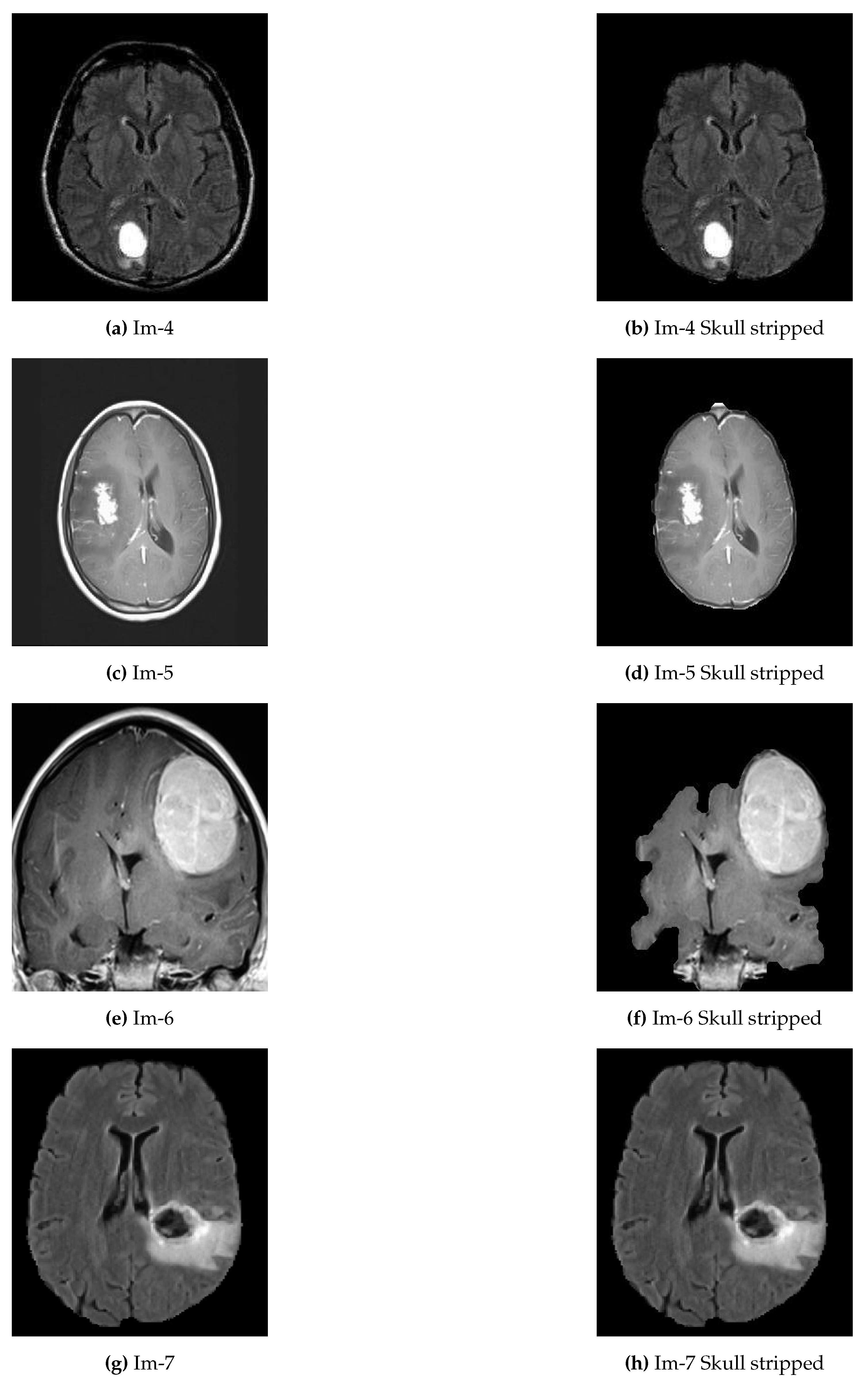
3.2. Preprocessing
| Algorithm 1 Skull Stripping |
|
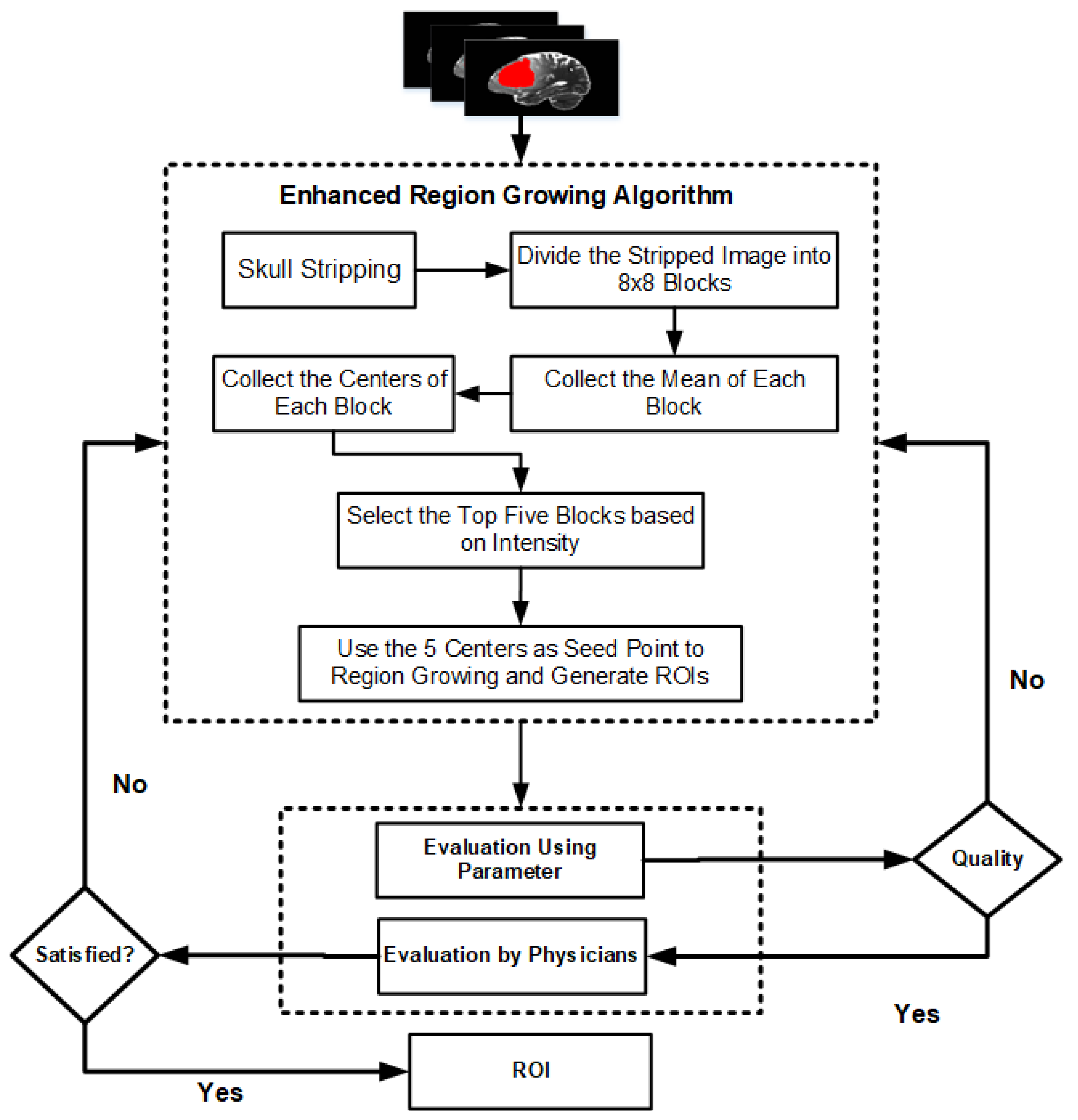
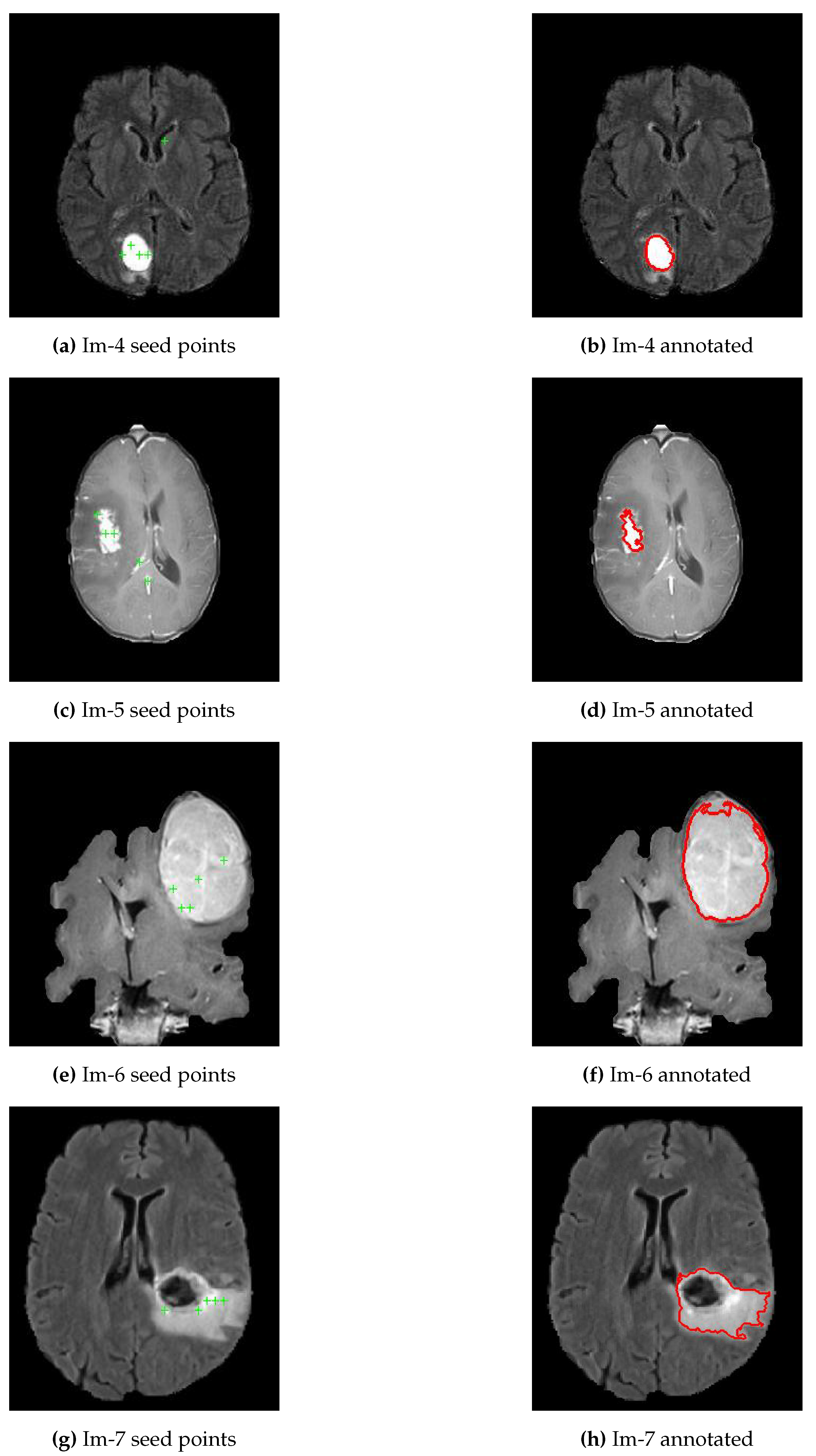
3.3. Enhanced Region-Growing Approach
| Algorithm 2 Enhanced Region Growing Segmentation for Brain Tumor Segmentation |
|
3.4. Evaluation Approach
3.4.1. Extra Fraction (EF)
3.4.2. Overlap Fraction (OF)
3.4.3. Dice Similarity Score (DSS)
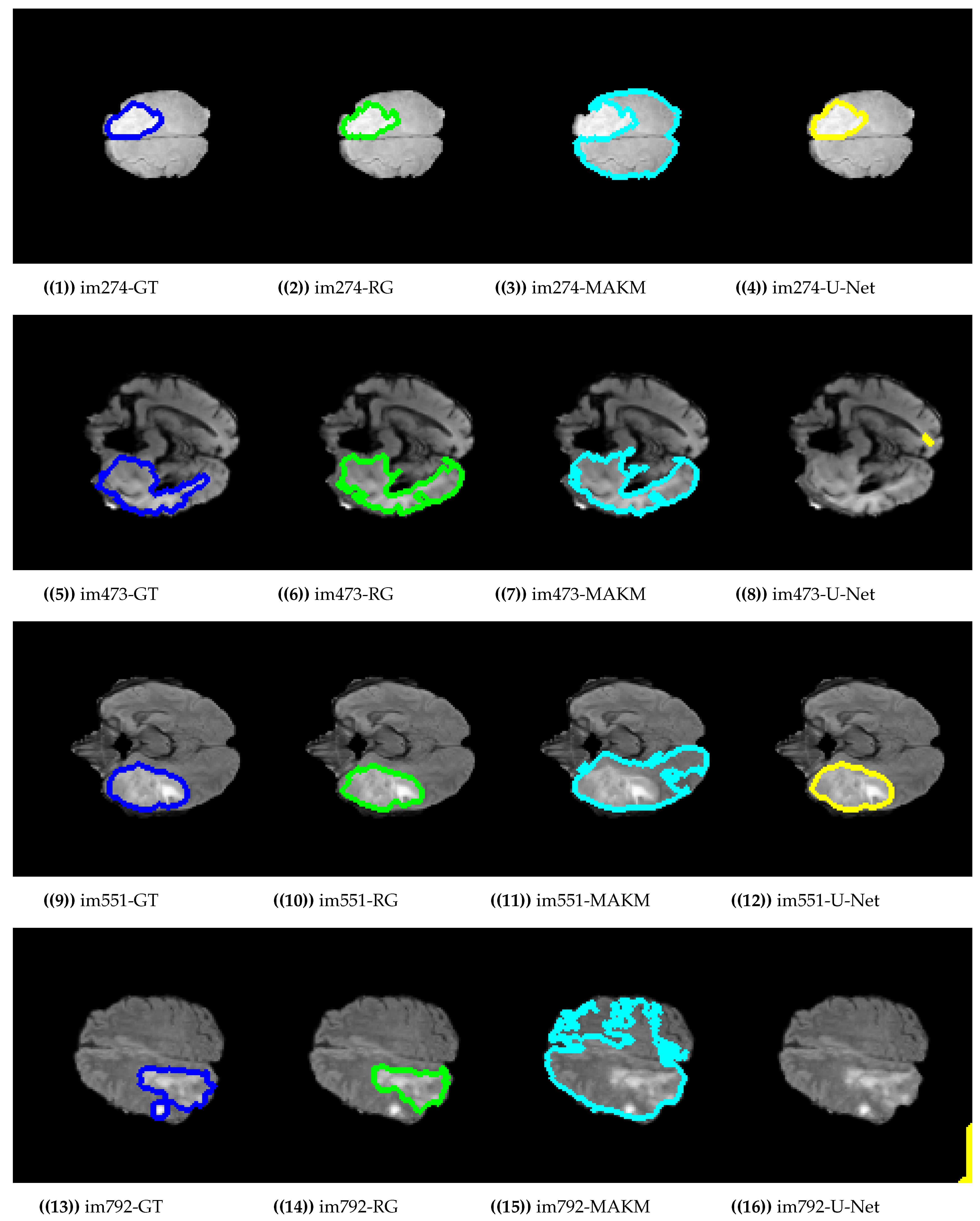
4. Experimental Results and Discussion
5. Conclusions
Author Contributions
Funding
Institutional Review Board Statement
Informed Consent Statement
Conflicts of Interest
References
- Sonar, P.; Bhosle, U.; Choudhury, C. Mammography classification using modified hybrid SVM-KNN. In Proceedings of the 2017 International Conference on Signal Processing and Communication (ICSPC), Coimbatore, India, 28–29 July 2017. [Google Scholar] [CrossRef]
- Yasiran, S.S.; Salleh, S.; Mahmud, R. Haralick texture and invariant moments features for breast cancer classification. AIP Conf. Proc. 2016, 1750, 020022. [Google Scholar]
- Aldape, K.; Brindle, K.M.; Chesler, L.; Chopra, R.; Gajjar, A.; Gilbert, M.R.; Gottardo, N.; Gutmann, D.H.; Hargrave, D.; Holland, E.C.; et al. Challenges to curing primary brain tumours. Nat. Rev. Clin. Oncol. 2019, 16, 509–520. [Google Scholar] [CrossRef] [PubMed] [Green Version]
- Zhao, Z.; Yang, G.; Lin, Y.; Pang, H.; Wang, M. Automated glioma detection and segmentation using graphical models. PLoS ONE 2018, 13, e0200745. [Google Scholar] [CrossRef] [PubMed] [Green Version]
- Birry, R.A.K. Automated Classification in Digital Images of Osteogenic Differentiated Stem Cells. Ph.D. Thesis, University of Salford, Salford, UK, 2013. [Google Scholar]
- Drevelegas, A.; Papanikolaou, N. Imaging modalities in brain tumors. In Imaging of Brain Tumors with Histological Correlations; Springer: Berlin/Heidelberg, Germany, 2011; pp. 13–33. [Google Scholar]
- Mechtler, L. Neuroimaging in Neuro-Oncology. Neurol. Clin. 2009, 27, 171–201. [Google Scholar] [CrossRef]
- Strong, M.J.; Garces, J.; Vera, J.C.; Mathkour, M.; Emerson, N.; Ware, M.L. Brain Tumors: Epidemiology and Current Trends in Treatment. J. Brain Tumors Neurooncol. 2015, 1, 1–21. [Google Scholar] [CrossRef]
- Mortazavi, D.; Kouzani, A.Z.; Soltanian-Zadeh, H. Segmentation of multiple sclerosis lesions in MR images: A review. Neuroradiology 2011, 54, 299–320. [Google Scholar] [CrossRef]
- Rundo, L.; Tangherloni, A.; Militello, C.; Gilardi, M.C.; Mauri, G. Multimodal medical image registration using Particle Swarm Optimization: A review. In Proceedings of the 2016 IEEE Symposium Series on Computational Intelligence (SSCI), Athens, Greece, 6–9 December 2016. [Google Scholar] [CrossRef]
- Balakrishnan, G.; Zhao, A.; Sabuncu, M.R.; Guttag, J.; Dalca, A.V. VoxelMorph: A Learning Framework for Deformable Medical Image Registration. IEEE Trans. Med. Imaging 2019, 38, 1788–1800. [Google Scholar] [CrossRef] [Green Version]
- MY-MS.org. MRI Basics. 2020. Available online: https://my-ms.org/mri_basics.htm (accessed on 1 October 2020).
- Stall, B.; Zach, L.; Ning, H.; Ondos, J.; Arora, B.; Shankavaram, U.; Miller, R.W.; Citrin, D.; Camphausen, K. Comparison of T2 and FLAIR imaging for target delineation in high grade gliomas. Radiat. Oncol. 2010, 5, 5. [Google Scholar] [CrossRef] [Green Version]
- Society, N.B.T. Quick Brain Tumor Facts. 2020. Available online: https://braintumor.org/brain-tumor-information/brain-tumor-facts/ (accessed on 3 October 2020).
- Rahimeto, S.; Debelee, T.; Yohannes, D.; Schwenker, F. Automatic pectoral muscle removal in mammograms. Evol. Syst. 2019. [Google Scholar] [CrossRef]
- Kebede, S.R.; Debelee, T.G.; Schwenker, F.; Yohannes, D. Classifier Based Breast Cancer Segmentation. J. Biomim. Biomater. Biomed. Eng. 2020, 47, 1–21. [Google Scholar]
- Cui, S.; Shen, X.; Lyu, Y. Automatic Segmentation of Brain Tumor Image Based on Region Growing with Co-constraint. In International Conference on Multimedia Modeling, Proceedings of the MMM 2019: MultiMedia Modeling, Thessaloniki, Greece, 8–11 January 2019; Springer: Berlin/Heidelberg, Germany, 2019; Volume 11295. [Google Scholar]
- Angulakshmi, M.; Lakshmi Priya, G.G. Automated Brain Tumour Segmentation Techniques—A Review. Int. J. Imaging Syst. Technol. 2017, 27, 66–77. [Google Scholar] [CrossRef] [Green Version]
- Rundo, L.; Tangherloni, A.; Cazzaniga, P.; Nobile, M.S.; Russo, G.; Gilardi, M.C.; Vitabile, S.; Mauri, G.; Besozzi, D.; Militello, C. A novel framework for MR image segmentation and quantification by using MedGA. Comput. Methods Programs Biomed. 2019, 176, 159–172. [Google Scholar] [CrossRef] [PubMed]
- Acharya, U.K.; Kumar, S. Particle swarm optimized texture based histogram equalization (PSOTHE) for MRI brain image enhancement. Optik 2020, 224, 165760. [Google Scholar] [CrossRef]
- Pandav, S. Brain tumor extraction using marker controlled watershed segmentation. Int. J. Eng. Res. Technol. 2014, 3, 2020–2022. [Google Scholar]
- Salman, Y. Validation techniques for quantitative brain tumors measurements. In Proceedings of the IEEE Engineering in Medicine and Biology 27th Annual Conference, Shanghai, China, 17–18 January 2006. [Google Scholar]
- Sarathi, M.P.; Ansari, M.G.A.; Uher, V.; Burget, R.; Dutta, M.K. Automated Brain Tumor segmentation using novel feature point detector and seeded region growing. In Proceedings of the 2013 36th International Conference on Telecommunications and Signal Processing (TSP), Rome, Italy, 2–4 July 2013; pp. 648–652. [Google Scholar]
- Thiruvenkadam, K.; Perumal, N. Brain Tumor Segmentation of MRI Brain Images through FCM clustering and Seeded Region Growing Technique. Int. J. Appl. Eng. Res. 2015, 10, 427–432. [Google Scholar]
- Ho, Y.L.; Lin, W.Y.; Tsai, C.L.; Lee, C.C.; Lin, C.Y. Automatic Brain Extraction for T1-Weighted Magnetic Resonance Images Using Region Growing. In Proceedings of the 2016 IEEE 16th International Conference on Bioinformatics and Bioengineering (BIBE), Taichung, Taiwan, 31 October–2 November 2016; pp. 250–253. [Google Scholar]
- Bauer, S.; Nolte, L.P.; Reyes, M. Fully Automatic Segmentation of Brain Tumor Images Using Support Vector Machine Classification in Combination with Hierarchical Conditional Random Field Regularization. In Lecture Notes in Computer Science; Springer: Berlin/Heidelberg, Germany, 2011; pp. 354–361. [Google Scholar] [CrossRef] [Green Version]
- Rundo, L.; Militello, C.; Tangherloni, A.; Russo, G.; Vitabile, S.; Gilardi, M.C.; Mauri, G. NeXt for neuro-radiosurgery: A fully automatic approach for necrosis extraction in brain tumor MRI using an unsupervised machine learning technique. Int. J. Imaging Syst. Technol. 2017, 28, 21–37. [Google Scholar] [CrossRef]
- Debelee, T.G.; Schwenker, F.; Ibenthal, A.; Yohannes, D. Survey of deep learning in breast cancer image analysis. Evol. Syst. 2019. [Google Scholar] [CrossRef]
- Debelee, T.G.; Gebreselasie, A.; Schwenker, F.; Amirian, M.; Yohannes, D. Classification of Mammograms Using Texture and CNN Based Extracted Features. J. Biomim. Biomater. Biomed. Eng. 2019, 42, 79–97. [Google Scholar] [CrossRef]
- Debelee, T.G.; Kebede, S.R.; Schwenker, F.; Shewarega, Z.M. Deep Learning in Selected Cancers’ Image Analysis—A Survey. J. Imaging 2020, 6, 121. [Google Scholar] [CrossRef]
- Afework, Y.K.; Debelee, T.G. Detection of Bacterial Wilt on Enset Crop Using Deep Learning Approach. Int. J. Eng. Res. Afr. 2020, 51, 131–146. [Google Scholar] [CrossRef]
- Debelee, T.G.; Amirian, M.; Ibenthal, A.; Palm, G.; Schwenker, F. Classification of Mammograms Using Convolutional Neural Network Based Feature Extraction. In Lecture Notes of the Institute for Computer Sciences, Social Informatics and Telecommunications Engineering; Springer: Cham, Switzerland, 2018; Volume 244, pp. 89–98. [Google Scholar]
- Li, Q.; Yu, Z.; Wang, Y.; Zheng, H. TumorGAN: A Multi-Modal Data Augmentation Framework for Brain Tumor Segmentation. Sensors 2020, 20, 4203. [Google Scholar] [CrossRef] [PubMed]
- Ibtehaz, N.; Rahman, M.S. MultiResUNet: Rethinking the U-Net architecture for multimodal biomedical image segmentation. Neural Netw. 2020, 121, 74–87. [Google Scholar] [CrossRef] [PubMed]
- Rundo, L.; Han, C.; Nagano, Y.; Zhang, J.; Hataya, R.; Militello, C.; Tangherloni, A.; Nobile, M.S.; Ferretti, C.; Besozzi, D.; et al. USE-Net: Incorporating Squeeze-and-Excitation blocks into U-Net for prostate zonal segmentation of multi-institutional MRI datasets. Neurocomputing 2019, 365, 31–43. [Google Scholar] [CrossRef] [Green Version]
- Kistler, M.; Bonaretti, S.; Pfahrer, M.; Niklaus, R.; Büchler, P. The Virtual Skeleton Database: An Open Access Repository for Biomedical Research and Collaboration. J. Med. Internet Res. 2013, 15, e245. [Google Scholar] [CrossRef] [Green Version]
- Menze, B.H.; Jakab, A.; Bauer, S.; Kalpathy-Cramer, J.; Farahani, K.; Kirby, J.; Burren, Y.; Porz, N.; Slotboom, J.; Wiest, R.; et al. The Multimodal Brain Tumor Image Segmentation Benchmark (BRATS). IEEE Trans. Med. Imaging 2014, 34, 1993–2024. [Google Scholar] [CrossRef]
- Zhao, J.; Meng, Z.; Wei, L.; Sun, C.; Zou, Q.; Su, R. Supervised Brain Tumor Segmentation Based on Gradient and Context-Sensitive Features. Front. Neurosci. 2019, 13, 1–11. [Google Scholar] [CrossRef]
- Reddy, B.; Reddy, P.B.; Kumar, P.S.; Reddy, S.S. Developing an Approach to Brain MRI Image Preprocessing for Tumor Detection. Int. J. Res. 2014, 1, 725–731. [Google Scholar]
- Ségonne, F.; Dale, A.M.; Busa, E.; Glessner, M.; Salat, D.; Hahn, H.K.; Fischl, B. A Hybrid Approach to the Skull Stripping Problem in MRI. Neuroimage 2004, 22, 1060–1075. [Google Scholar] [CrossRef]
- Vishnuvarthanan, G.; Rajasekaran, M.P.; Vishnuvarthanan, N.A.; Prasath, T.A.; Kannan, M. Tumor Detection in T1, T2, FLAIR and MPR Brain Images Using a Combination of Optimization and Fuzzy Clustering Improved by Seed-Based Region Growing Algorithm. Int. J. Imaging Syst. Technol. 2017, 27, 33–45. [Google Scholar] [CrossRef] [Green Version]
- Daimary, D.; Bora, M.B.; Amitab, K.; Kandar, D. Brain Tumor Segmentation from MRI Images using Hybrid Convolutional Neural Networks. Procedia Comput. Sci. 2020, 167, 2419–2428. [Google Scholar] [CrossRef]
- Havaei, M.; Dutil, F.; Pal, C.; Larochelle, H.; Jodoin, P.M. A Convolutional Neural Network Approach to Brain Tumor Segmentation. In Brainlesion: Glioma, Multiple Sclerosis, Stroke and Traumatic Brain Injuries; Springer: Cham, Switzerland, 2016; pp. 195–208. [Google Scholar] [CrossRef]
- Pereira, S.; Pinto, A.; Alves, V.; Silva, C.A. Deep Convolutional Neural Networks for the Segmentation of Gliomas in Multi-sequence MRI. In Brainlesion: Glioma, Multiple Sclerosis, Stroke and Traumatic Brain Injuries; Springer: Cham, Switzerland, 2016; pp. 131–143. [Google Scholar] [CrossRef]
- Malmi, E.; Parambath, S.; Peyrat, J.M.; Abinahed, J.; Chawla, S. CaBS: A Cascaded Brain Tumor Segmentation Approach. Proc. MICCAI Brain Tumor Segmentation (BRATS) 2015, 42–47. Available online: http://www2.imm.dtu.dk/projects/BRATS2012/proceedingsBRATS2012.pdf (accessed on 8 August 2020).
- Debelee, T.G.; Schwenker, F.; Rahimeto, S.; Yohannes, D. Evaluation of modified adaptive k-means segmentation algorithm. Comput. Vis. Media 2019. [Google Scholar] [CrossRef] [Green Version]
- Dong, H.; Yang, G.; Liu, F.; Mo, Y.; Guo, Y. Automatic Brain Tumor Detection and Segmentation Using U-Net Based Fully Convolutional Networks. In Communications in Computer and Information Science; Springer: Cham, Switzerland, 2017; pp. 506–517. [Google Scholar] [CrossRef] [Green Version]


| Authors and Citation | Seed Selection | RG Criteria |
|---|---|---|
| Salman et al., 2006 [22] | Manual | Texture |
| Sarathi et al., 2013 [23] | Automatic | variance, Entropy |
| Thiruvenkadam, 2015 [24] | Manual | - |
| Ho et al., 2016 [25] | Automatic | Intensity |
| Cui et al., 2019 [17] | Semi-automatic | Intensity & Spatial Texture |
| Metric | Algorithm | im01 | im02 | im03 | im04 | im05 | im06 | im07 | im08 | im09 | im10 | im11 | im12 | im13 | im14 | im15 | Avg |
|---|---|---|---|---|---|---|---|---|---|---|---|---|---|---|---|---|---|
| RG | 100 | 100 | 100 | 100 | 99 | 99 | 99 | 99 | 99 | 99 | 100 | 99 | 99 | 88 | 94 | 98 | |
| Acc (%) | MAKM | 99 | 99 | 99 | 82 | 99 | 99 | 99 | 99 | 86 | 86 | 80 | 87 | 99 | 87 | 99 | 93 |
| U-Net | 100 | 100 | 100 | 100 | 98 | 98 | 74 | 74 | 99 | 99 | 67 | 99 | 100 | 99 | 92 | 93 | |
| RG | 0.94 | 0.94 | 0.94 | 0.93 | 0.88 | 0.88 | 0.85 | 0.85 | 0.85 | 0.85 | 0.84 | 0.83 | 0.81 | 0.31 | 0.04 | 0.78 | |
| IoU | MAKM | 0.90 | 0.79 | 0.79 | 0.21 | 0.86 | 0.86 | 0.90 | 0.90 | 0.26 | 0.26 | 0.06 | 0.19 | 0.81 | 0.34 | 0.65 | 0.59 |
| U-Net | 0.94 | 0.96 | 0.96 | 0.93 | 0.70 | 0.70 | 0.16 | 0.16 | 0.91 | 0.91 | 0.03 | 0.84 | 0.93 | 0.81 | 0.24 | 0.68 | |
| RG | 0.97 | 0.97 | 0.97 | 0.96 | 0.93 | 0.93 | 0.92 | 0.92 | 0.92 | 0.92 | 0.91 | 0.91 | 0.89 | 0.47 | 0.80 | 0.89 | |
| DSS | MAKM | 0.95 | 0.88 | 0.88 | 0.35 | 0.92 | 0.92 | 0.95 | 0.95 | 0.42 | 0.42 | 0.11 | 0.33 | 0.90 | 0.51 | 0.79 | 0.68 |
| U-Net | 0.97 | 0.98 | 0.98 | 0.96 | 0.82 | 0.82 | 0.27 | 0.27 | 0.95 | 0.95 | 0.07 | 0.92 | 0.96 | 0.89 | 0.39 | 0.75 | |
| RG | 97 | 95 | 95 | 98 | 88 | 88 | 87 | 87 | 85 | 85 | 85 | 83 | 81 | 100 | 100 | 90 | |
| Sn (%) | MAKM | 91 | 79 | 79 | 100 | 86 | 86 | 96 | 96 | 100 | 100 | 100 | 99 | 85 | 100 | 65 | 91 |
| U-Net | 100 | 98 | 98 | 93 | 95 | 95 | 99 | 99 | 100 | 100 | 90 | 100 | 96 | 88 | 65 | 94 | |
| RG | 100 | 100 | 100 | 100 | 100 | 100 | 100 | 100 | 100 | 100 | 100 | 100 | 100 | 84 | 00 | 92 | |
| Sp (%) | MAKM | 100 | 100 | 100 | 81 | 100 | 100 | 100 | 100 | 85 | 85 | 79 | 86 | 100 | 86 | 100 | 93 |
| U-Net | 100 | 100 | 100 | 100 | 98 | 98 | 73 | 73 | 99 | 99 | 67 | 99 | 100 | 99 | 93 | 93 | |
| RG | 0.03 | 0.02 | 0.02 | 0.06 | 0.00 | 0.00 | 0.02 | 0.02 | 0.00 | 0.00 | 0.01 | 0.00 | 0.00 | 2.27 | 23.37 | 1.72 | |
| EF | MAKM | 0.01 | 0.00 | 0.00 | 3.79 | 0.00 | 0.00 | 0.06 | 0.06 | 2.79 | 2.79 | 16.11 | 4.09 | 0.04 | 1.92 | 0.00 | 2.11 |
| U-Net | 0.05 | 0.02 | 0.02 | 0.00 | 0.35 | 0.35 | 5.23 | 5.23 | 0.10 | 0.10 | 25.57 | 0.18 | 0.03 | 0.08 | 1.69 | 2.60 | |
| RG | 0.97 | 0.95 | 0.95 | 0.98 | 0.88 | 0.88 | 0.87 | 0.87 | 0.85 | 0.85 | 0.85 | 0.83 | 0.81 | 1.00 | 1.00 | 0.90 | |
| OF | MAKM | 0.91 | 0.79 | 0.79 | 1.00 | 0.86 | 0.86 | 0.96 | 0.96 | 1.00 | 1.00 | 1.00 | 0.99 | 0.85 | 1.00 | 0.65 | 0.91 |
| U-Net | 1.00 | 0.98 | 0.98 | 0.93 | 0.95 | 0.95 | 0.99 | 0.99 | 1.00 | 1.00 | 0.90 | 1.00 | 0.96 | 0.88 | 0.65 | 0.94 | |
| RG | 72.72 | 74.40 | 74.40 | 72.72 | 70.22 | 70.22 | 69.50 | 69.50 | 69.38 | 69.38 | 75.09 | 70.79 | 68.25 | 56.31 | 48.31 | 68.75 | |
| PSNR | MAKM | 70.63 | 69.38 | 69.38 | 55.51 | 69.67 | 69.67 | 71.02 | 71.02 | 56.66 | 56.66 | 55.02 | 56.88 | 68.19 | 57.03 | 66.53 | 64.22 |
| U-Net | 72.99 | 76.49 | 76.49 | 72.64 | 65.12 | 65.12 | 54.06 | 54.06 | 71.02 | 71.02 | 53.00 | 70.37 | 72.64 | 66.70 | 58.92 | 66.71 |
| Metric | Algorithm | im081 | im274 | im473 | im551 | im06 | im973 | im689 | im792 | im1507 | im781 | im733 | im1238 | Avg |
|---|---|---|---|---|---|---|---|---|---|---|---|---|---|---|
| RG | 99.6 | 99.8 | 97.4 | 99.6 | 99.6 | 99.7 | 100.0 | 99.1 | 98.7 | 99.2 | 99.7 | 96.8 | 99.1 | |
| Acc (%) | MAKM | 84.9 | 89.1 | 97.2 | 95.9 | 85.4 | 79.7 | 76.9 | 87.7 | 84.3 | 95.6 | 90.4 | 84.6 | 87.6 |
| U-NET | 99.8 | 99.8 | 93.3 | 99.8 | 99.8 | 98.7 | 99.8 | 89.2 | 99.5 | 99.5 | 99.1 | 86.6 | 97.1 | |
| RG | 0.91 | 0.92 | 0.62 | 0.92 | 0.92 | 0.94 | 0.89 | 0.77 | 0.80 | 0.88 | 0.85 | 0.47 | 0.82 | |
| IoU | MAKM | 0.05 | 0.01 | 0.61 | 0.50 | 0.23 | 0.02 | 0.02 | 0.23 | 0.29 | 0.58 | 0.04 | 0.28 | 0.24 |
| U-NET | 0.95 | 0.93 | 0.39 | 0.94 | 0.95 | 0.76 | 0.61 | 0.25 | 0.92 | 0.93 | 0.45 | 0.31 | 0.70 | |
| RG | 0.95 | 0.96 | 0.76 | 0.96 | 0.96 | 0.97 | 0.94 | 0.87 | 0.89 | 0.94 | 0.92 | 0.64 | 0.90 | |
| DSS | MAKM | 0.09 | 0.01 | 0.75 | 0.67 | 0.38 | 0.03 | 0.03 | 0.37 | 0.44 | 0.74 | 0.09 | 0.44 | 0.34 |
| U-NET | 0.98 | 0.96 | 0.56 | 0.97 | 0.97 | 0.86 | 0.76 | 0.40 | 0.96 | 0.96 | 0.62 | 0.47 | 0.79 | |
| RG | 95.3 | 93.9 | 83.5 | 92.1 | 94.5 | 96.2 | 92.2 | 82.0 | 79.8 | 91.2 | 92.9 | 46.8 | 86.7 | |
| Sn (%) | MAKM | 18.2 | 3.5 | 89.1 | 99.3 | 100.0 | 7.4 | 100.0 | 96.9 | 99.4 | 99.9 | 25.8 | 98.5 | 69.8 |
| U-NET | 98.9 | 97.7 | 85.7 | 98.0 | 98.8 | 97.2 | 60.9 | 98.3 | 92.9 | 95.4 | 45.2 | 99.9 | 89.1 | |
| RG | 99.8 | 100.0 | 98.2 | 100.0 | 99.9 | 99.9 | 100.0 | 99.8 | 100.0 | 99.8 | 99.8 | 100.0 | 99.7 | |
| Sp (%) | MAKM | 87.9 | 90.9 | 97.6 | 95.7 | 84.7 | 82.9 | 76.8 | 87.4 | 83.3 | 95.3 | 91.6 | 83.7 | 88.2 |
| U-NET | 99.8 | 99.9 | 93.7 | 99.8 | 99.8 | 98.8 | 100.0 | 88.9 | 99.9 | 99.8 | 100.0 | 85.8 | 97.2 | |
| RG | 0.05 | 0.02 | 0.35 | 0.01 | 0.03 | 0.02 | 0.03 | 0.06 | 0.00 | 0.03 | 0.09 | 0.00 | 0.06 | |
| EF | MAKM | 0.18 | 0.03 | 0.89 | 0.99 | 1.00 | 0.07 | 1.00 | 0.97 | 0.99 | 1.00 | 0.26 | 0.98 | 0.70 |
| U-NET | 0.99 | 0.98 | 0.86 | 0.98 | 0.99 | 0.97 | 0.61 | 0.98 | 0.93 | 0.95 | 0.45 | 1.00 | 0.89 | |
| RG | 0.95 | 0.94 | 0.83 | 0.92 | 0.94 | 0.96 | 0.92 | 0.82 | 0.80 | 0.91 | 0.93 | 0.47 | 0.87 | |
| OF | MAKM | 0.18 | 0.03 | 0.89 | 0.99 | 1.00 | 0.07 | 1.00 | 0.97 | 0.99 | 1.00 | 0.26 | 0.98 | 0.70 |
| U-NET | 0.99 | 0.98 | 0.86 | 0.98 | 0.99 | 0.97 | 0.61 | 0.98 | 0.93 | 0.95 | 0.45 | 1.00 | 0.89 | |
| RG | 165.52 | 174.19 | 147.51 | 167.26 | 166.43 | 170.25 | 188.41 | 157.89 | 154.39 | 159.74 | 169.80 | 145.23 | 163.89 | |
| PNSR | MAKM | 129.72 | 132.99 | 146.42 | 142.69 | 130.06 | 126.75 | 125.49 | 131.81 | 129.36 | 142.02 | 134.30 | 129.55 | 133.43 |
| U-NET | 172.31 | 175.68 | 137.87 | 170.98 | 171.49 | 154.11 | 175.68 | 133.12 | 163.80 | 164.69 | 157.43 | 130.96 | 159.01 |
| Metric | Algorithm | im081 | im274 | im473 | im551 | im06 | im973 | im689 | im792 | im1507 | im781 | im733 | im1238 | im368 | … | im551 | Ovr_Avg |
|---|---|---|---|---|---|---|---|---|---|---|---|---|---|---|---|---|---|
| RG | 99.6 | 99.8 | 97.4 | 99.6 | 99.6 | 99.7 | 100.0 | 99.1 | 98.7 | 99.2 | 99.7 | 96.8 | 95.2 | … | 97.8 | 98.72 | |
| Acc (%) | MAKM | 84.9 | 89.1 | 97.2 | 95.9 | 85.4 | 79.7 | 76.9 | 87.7 | 84.3 | 95.6 | 90.4 | 84.6 | 98.8 | … | 98.7 | 88.60 |
| U-NET | 99.8 | 99.8 | 93.3 | 99.8 | 99.8 | 98.7 | 99.8 | 89.2 | 99.5 | 99.5 | 77.6 | 86.6 | 83.8 | … | 99.8 | 98.20 | |
| RG | 0.91 | 0.92 | 0.62 | 0.92 | 0.92 | 0.94 | 0.89 | 0.77 | 0.80 | 0.88 | 0.85 | 0.47 | 0.28 | … | 0.77 | 0.67 | |
| IoU | MAKM | 0.05 | 0.01 | 0.61 | 0.50 | 0.23 | 0.02 | 0.02 | 0.23 | 0.29 | 0.58 | 0.04 | 0.28 | 0.81 | … | 0.85 | 0.34 |
| U-NET | 0.95 | 0.93 | 0.39 | 0.94 | 0.95 | 0.76 | 0.61 | 0.25 | 0.92 | 0.93 | 0.45 | 0.31 | 0.26 | … | 0.27 | 0.60 | |
| RG | 0.95 | 0.96 | 0.76 | 0.96 | 0.96 | 0.97 | 0.94 | 0.87 | 0.89 | 0.94 | 0.92 | 0.87 | 0.43 | … | 0.96 | 0.80 | |
| DSS | MAKM | 0.09 | 0.01 | 0.75 | 0.67 | 0.38 | 0.03 | 0.03 | 0.37 | 0.44 | 0.74 | 0.09 | 0.34 | 0.90 | … | 0.92 | 0.45 |
| U-NET | 0.98 | 0.96 | 0.56 | 0.97 | 0.97 | 0.86 | 0.76 | 0.40 | 0.96 | 0.96 | 0.62 | 0.47 | 0.42 | … | 0.43 | 0.69 | |
| RG | 95.3 | 93.9 | 83.5 | 92.1 | 94.5 | 96.2 | 92.2 | 82.0 | 79.8 | 91.2 | 92.9 | 46.8 | 26.8 | … | 76.7 | 71.1 | |
| Sn (%) | MAKM | 18.2 | 3.5 | 89.1 | 99.3 | 100.0 | 7.4 | 100.0 | 96.9 | 99.4 | 99.9 | 25.8 | 98.5 | 82.4 | … | 85.5 | 89.6 |
| U-NET | 98.9 | 97.7 | 85.7 | 98.0 | 98.8 | 97.2 | 60.9 | 98.3 | 92.9 | 95.4 | 45.2 | 99.9 | 89.4 | … | 97.8 | 90.7 | |
| RG | 99.8 | 100.0 | 98.2 | 100.0 | 99.9 | 99.9 | 100.0 | 99.8 | 100.0 | 99.8 | 99.8 | 100.0 | 100 | … | 100 | 99.8 | |
| Sp (%) | MAKM | 87.9 | 90.9 | 97.6 | 95.7 | 84.7 | 82.9 | 76.8 | 87.4 | 83.3 | 95.3 | 91.6 | 83.7 | 100 | … | 100 | 88.6 |
| U-NET | 99.8 | 99.9 | 93.7 | 99.8 | 99.8 | 98.8 | 100.0 | 88.9 | 99.9 | 99.8 | 100.0 | 85.8 | 83.5 | … | 75.7 | 92.1 | |
| RG | 0.05 | 0.02 | 0.35 | 0.01 | 0.03 | 0.02 | 0.03 | 0.06 | 0.00 | 0.03 | 0.09 | 0.00 | 0 | … | 0 | 0.06 | |
| EF | MAKM | 0.18 | 0.03 | 0.89 | 0.99 | 1.00 | 0.07 | 1.00 | 0.97 | 0.99 | 1.00 | 0.26 | 0.98 | 0.82 | … | 0.85 | 0.90 |
| U-NET | 0.99 | 0.98 | 0.86 | 0.98 | 0.99 | 0.97 | 0.61 | 0.98 | 0.93 | 0.95 | 0.45 | 1.00 | 0.89 | … | 0.98 | 0.91 | |
| RG | 0.95 | 0.94 | 0.83 | 0.92 | 0.94 | 0.96 | 0.92 | 0.82 | 0.80 | 0.91 | 0.93 | 0.47 | 0.27 | … | 0.77 | 0.71 | |
| OF | MAKM | 0.18 | 0.03 | 0.89 | 0.99 | 1.00 | 0.07 | 1.00 | 0.97 | 0.99 | 1.00 | 0.26 | 0.98 | 0.82 | … | 0.85 | 0.90 |
| U-NET | 0.99 | 0.98 | 0.86 | 0.98 | 0.99 | 0.97 | 0.61 | 0.98 | 0.93 | 0.95 | 0.45 | 1.00 | 0.89 | … | 0.98 | 0.91 | |
| RG | 165.52 | 174.19 | 147.51 | 167.26 | 166.43 | 170.25 | 188.41 | 157.89 | 154.39 | 159.74 | 169.80 | 145.23 | 141.3 | … | 149.8 | 157.0 | |
| PNSR | MAKM | 129.72 | 132.99 | 146.42 | 142.69 | 130.06 | 126.75 | 125.49 | 131.81 | 129.36 | 142.02 | 134.30 | 129.55 | 155.0 | … | 154.1 | 138.6 |
| U-NET | 172.31 | 175.68 | 137.87 | 170.98 | 171.49 | 154.11 | 175.68 | 133.12 | 163.80 | 164.69 | 157.43 | 130.96 | 129.1 | … | 125.8 | 152.0 |
| Authors, Year and Citation | Model | Dataset | DSS |
|---|---|---|---|
| Daimary et al. [42] | U-SegNet | BRATS2015 | 0.73 |
| Zhou et al., 2019 | OM-Net + CGAp | BRATS2015 | 0.87 |
| Kayalibay et al., 2017 | CNN + 3D filters | BRATS2015 | 0.85 |
| Isensee et al., 2018 | U-Net + more filters | BRATS2015 | 0.85 |
| + data augmentation | |||
| + dice-loss | |||
| Kamnitsas et al., 2016 | 3D CNN + CRF | BRATS2015 | 0.85 |
| Qin et al., 2018 | AFN-6 | BRATS2015 | 0.84 |
| Havaei et al. [43] | CNN(whole) | BRATS2015 | 0.88 |
| Havaei et al. [43] | CNN(core) | BRATS2015 | 0.79 |
| Havaei et al. [43] | CNN(enhanced) | BRATS2015 | 0.73 |
| Pereira et al. [44] | CNN(whole) | BRATS2015 | 0.87 |
| Pereira et al. [44] | CNN(core) | BRATS2015 | 0.73 |
| Pereira et al. [44] | CNN(enhanced) | BRATS2015 | 0.68 |
| Malmi et al. [45] | CNN(whole) | BRATS2015 | 0.80 |
| Malmi et al. [45] | CNN(core) | BRATS2015 | 0.71 |
| Malmi et al. [45] | CNN(enhanced) | BRATS2015 | 0.64 |
| Taye et al., 2018 [46] | MAKM | BRATS2015 | 0.68 |
| Re-implemented | U-Net | BRATS2015 | 0.75 |
| Erena et al., 2020 | Case-1:Proposed Approach (15 randomly selected images) | BRATS2015 | 0.89 |
| Erena et al., 2020 | Case-2:Proposed Approach (12 randomly selected images) | BRATS2015 | 0.90 |
| Erena et al., 2020 | Case-3:Proposed Approach (800 brain images) | BRATS2015 | 0.80 |
| Erena et al., 2020 | Average:Proposed Approach | BRATS2015 | 0.86 |
Publisher’s Note: MDPI stays neutral with regard to jurisdictional claims in published maps and institutional affiliations. |
© 2021 by the authors. Licensee MDPI, Basel, Switzerland. This article is an open access article distributed under the terms and conditions of the Creative Commons Attribution (CC BY) license (http://creativecommons.org/licenses/by/4.0/).
Share and Cite
Biratu, E.S.; Schwenker, F.; Debelee, T.G.; Kebede, S.R.; Negera, W.G.; Molla, H.T. Enhanced Region Growing for Brain Tumor MR Image Segmentation. J. Imaging 2021, 7, 22. https://0-doi-org.brum.beds.ac.uk/10.3390/jimaging7020022
Biratu ES, Schwenker F, Debelee TG, Kebede SR, Negera WG, Molla HT. Enhanced Region Growing for Brain Tumor MR Image Segmentation. Journal of Imaging. 2021; 7(2):22. https://0-doi-org.brum.beds.ac.uk/10.3390/jimaging7020022
Chicago/Turabian StyleBiratu, Erena Siyoum, Friedhelm Schwenker, Taye Girma Debelee, Samuel Rahimeto Kebede, Worku Gachena Negera, and Hasset Tamirat Molla. 2021. "Enhanced Region Growing for Brain Tumor MR Image Segmentation" Journal of Imaging 7, no. 2: 22. https://0-doi-org.brum.beds.ac.uk/10.3390/jimaging7020022