Author Contributions
Conceptualization, M.K., M.M., and A.J.; methodology, M.K., M.M., and A.J.; validation, M.K., M.M., T.R., and J.-P.V.; formal analysis, M.K. and M.M.; investigation, M.K., M.M., and T.R.; resources, H.H. and M.T.V.; writing—original draft preparation, M.K., M.M., A.J., T.R., J.-P.V.; writing—review and editing, M.K., M.M., A.J., T.R., J.-P.V., J.H., M.T.V., and H.H.; visualization, M.K., M.M., and T.R.; project administration H.H. and M.T.V.; funding acquisition, M.T.V., J.-P.V., J.H., and H.H. All authors have read and agreed to the published version of the manuscript.
Figure 1.
Time-of-flight scanner Leica RTC360.
Figure 1.
Time-of-flight scanner Leica RTC360.
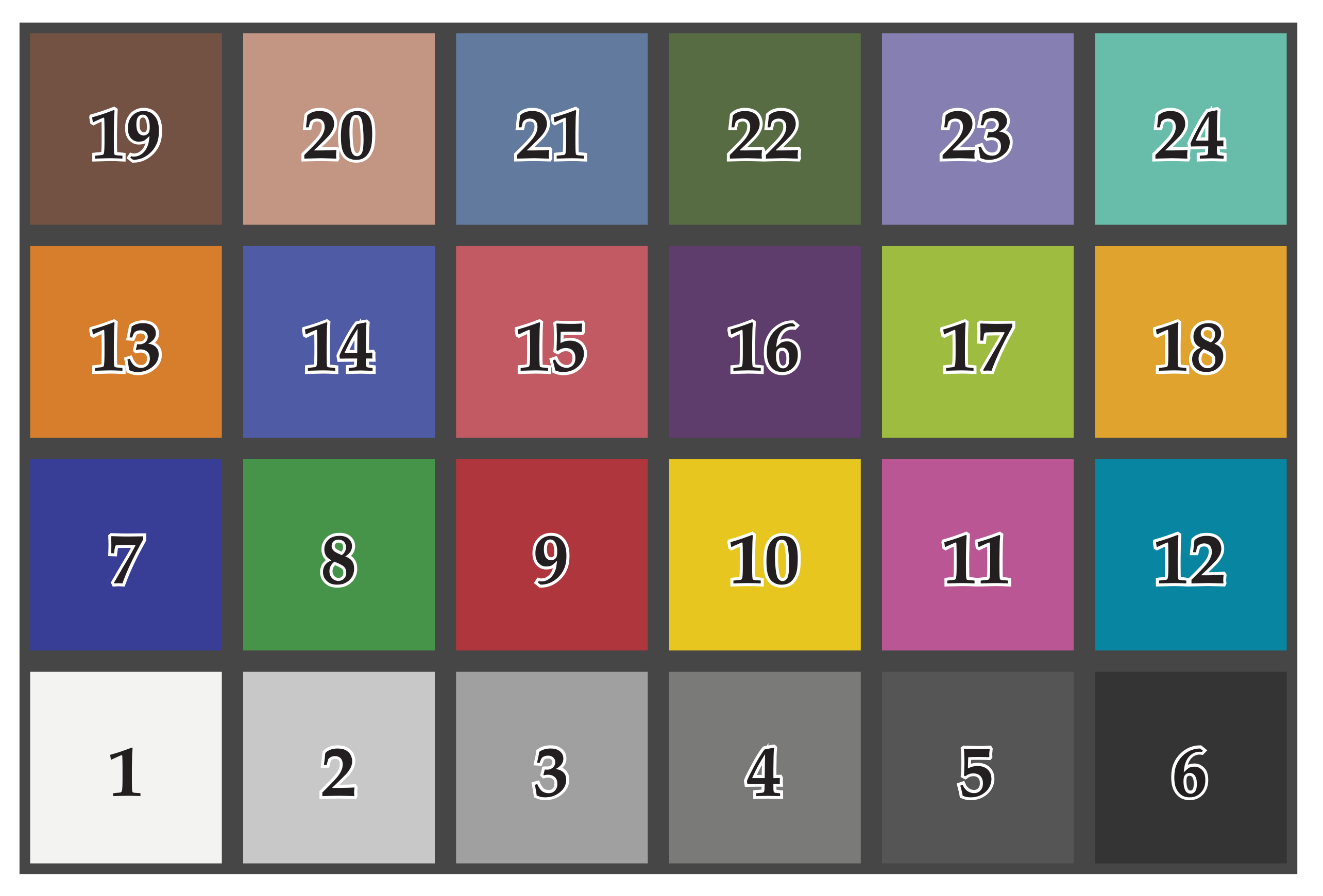
Figure 2.
The measured target X-Rite ColorChecker Classic and the patch numbers used in this study.
Figure 2.
The measured target X-Rite ColorChecker Classic and the patch numbers used in this study.
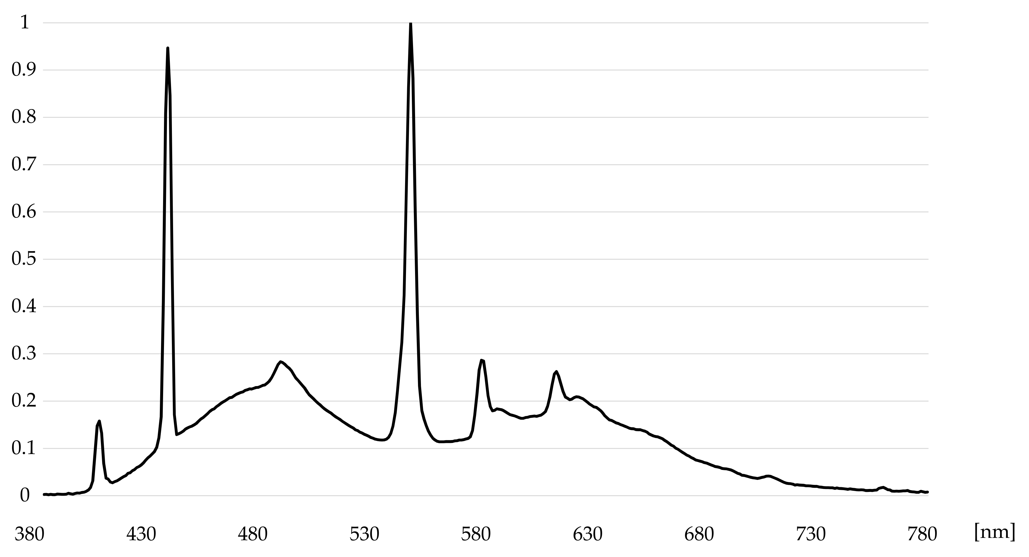
Figure 3.
The normalized spectral power function of patch No. 1.
Figure 3.
The normalized spectral power function of patch No. 1.
Figure 4.
The CIE color matching functions , , .
Figure 4.
The CIE color matching functions , , .
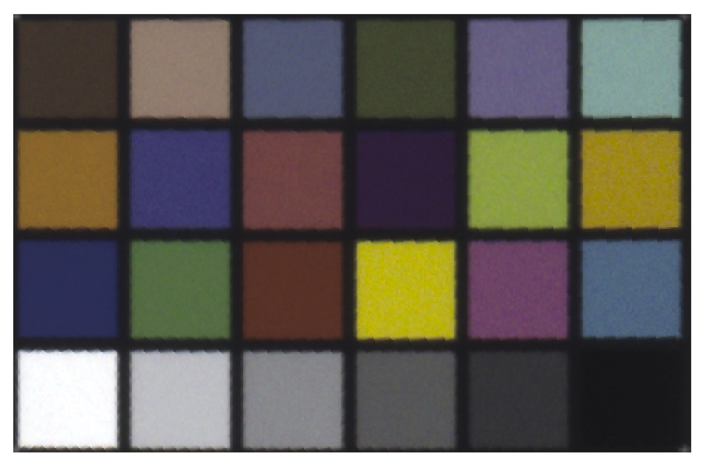
Figure 5.
The color target cropped from the panoramic image captured with the TLS instrument.
Figure 5.
The color target cropped from the panoramic image captured with the TLS instrument.
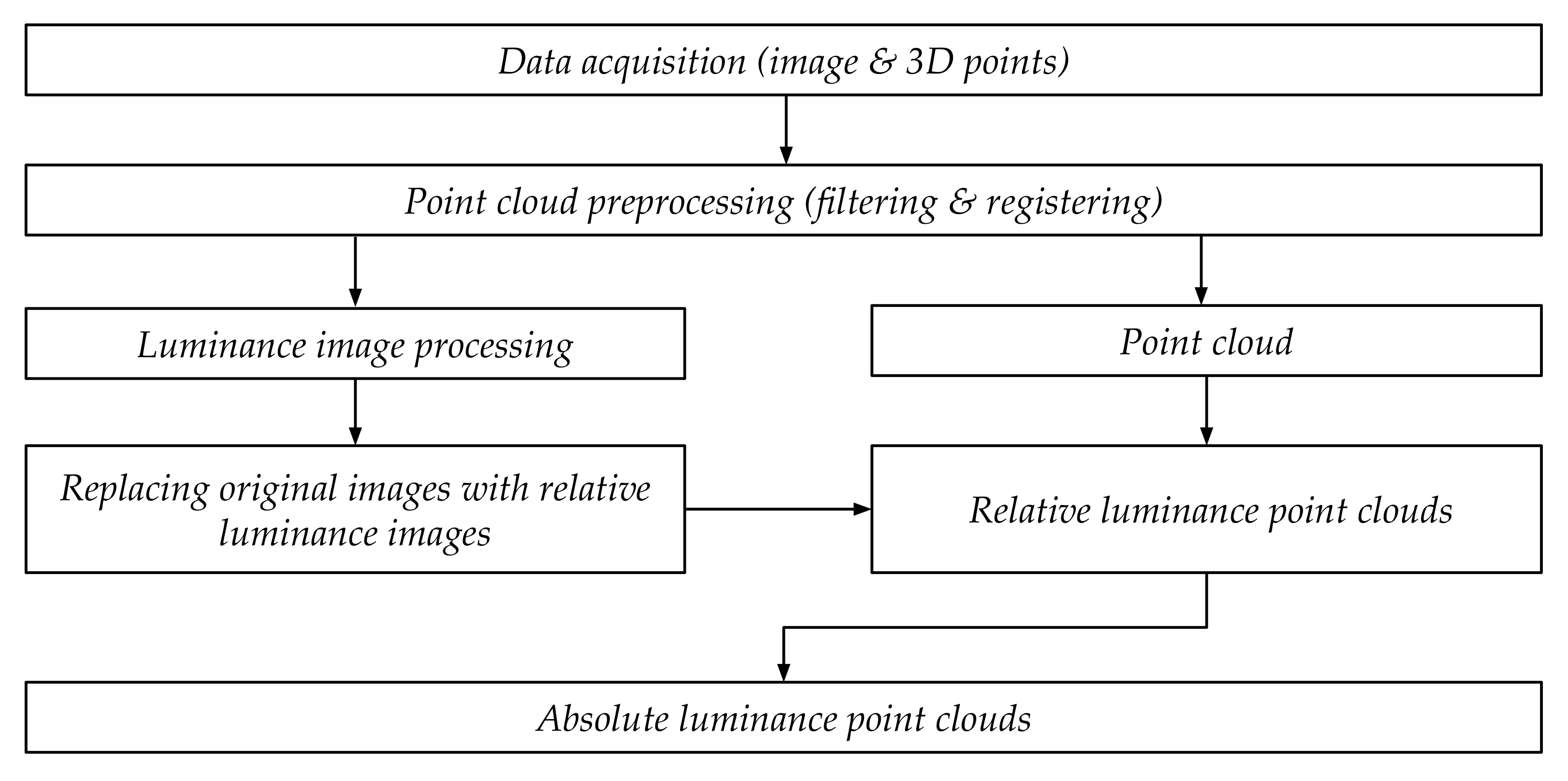
Figure 6.
The workflow for creating data for indoor 3D luminance maps.
Figure 6.
The workflow for creating data for indoor 3D luminance maps.
Figure 7.
The 360 panoramic image taken with the TLS instrument.
Figure 7.
The 360 panoramic image taken with the TLS instrument.
Figure 8.
The intensity image from scanning station 6 shows the locations of the sample areas for luminance measurements. The green areas represent the sample areas A–G. The red area represents the vertical sample area. The yellow area represents the horizontal sample area. White points represent the 6 different scanning locations with the seventh scanning location being the observer of the image.
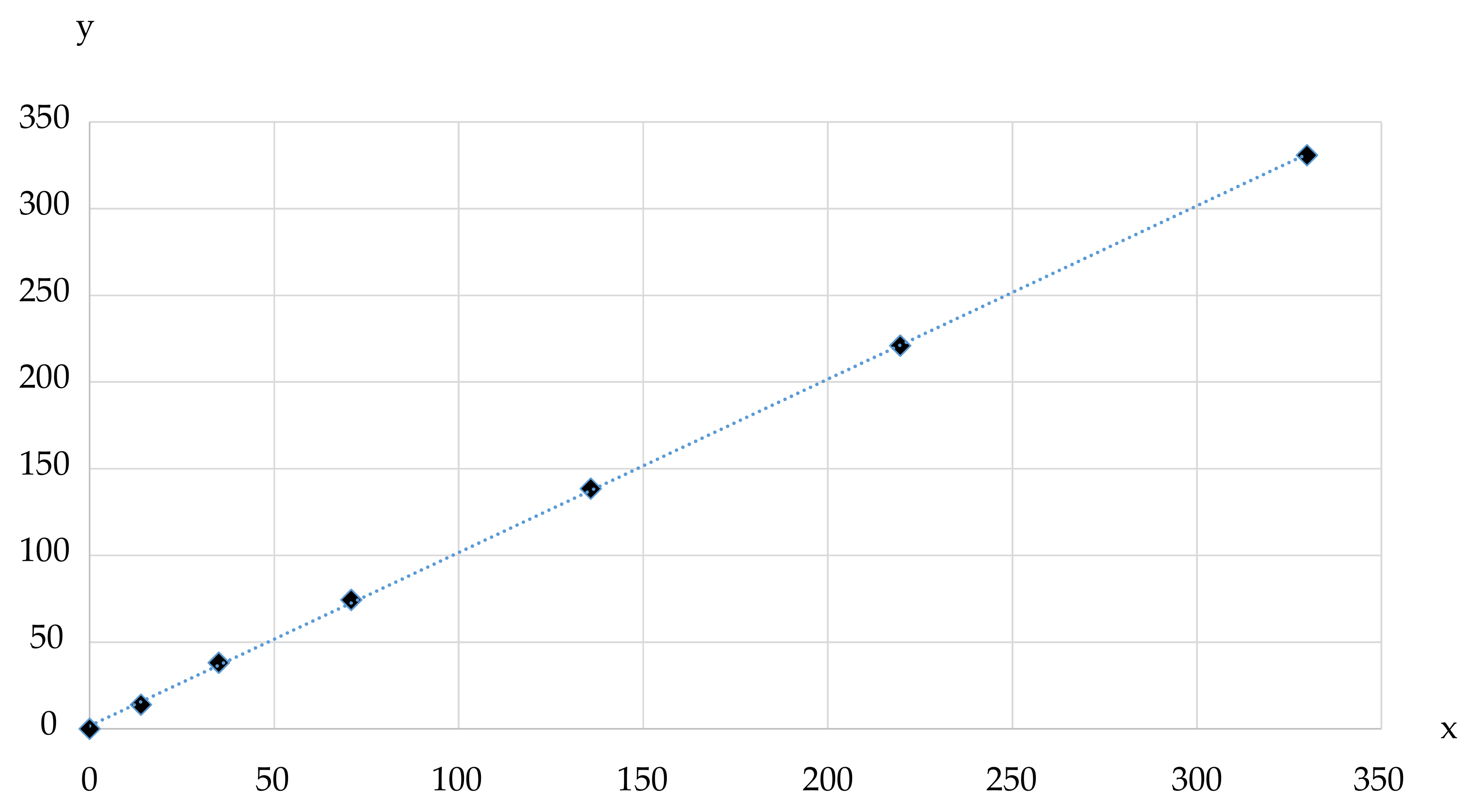
Figure 9.
The TLS luminance measurement (y) presented as a function of the reference luminance measurement (x) and its linear trendline.
Figure 9.
The TLS luminance measurement (y) presented as a function of the reference luminance measurement (x) and its linear trendline.
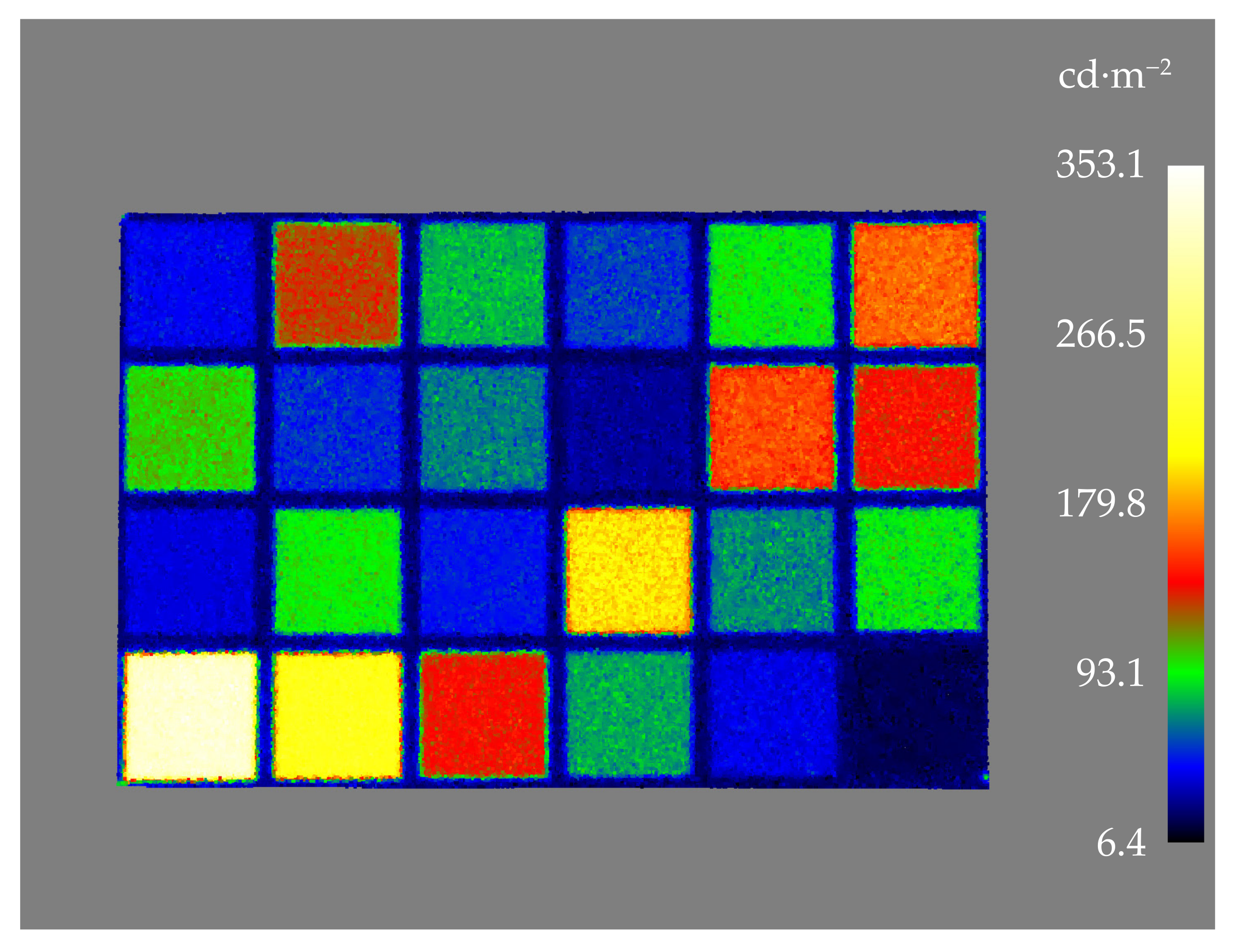
Figure 10.
Luminances of the measured color target X-Rite ColorChecker Classic. The patches in the lowest row of patches (1–6) are the grayscale patches used for luminance calibration.
Figure 10.
Luminances of the measured color target X-Rite ColorChecker Classic. The patches in the lowest row of patches (1–6) are the grayscale patches used for luminance calibration.
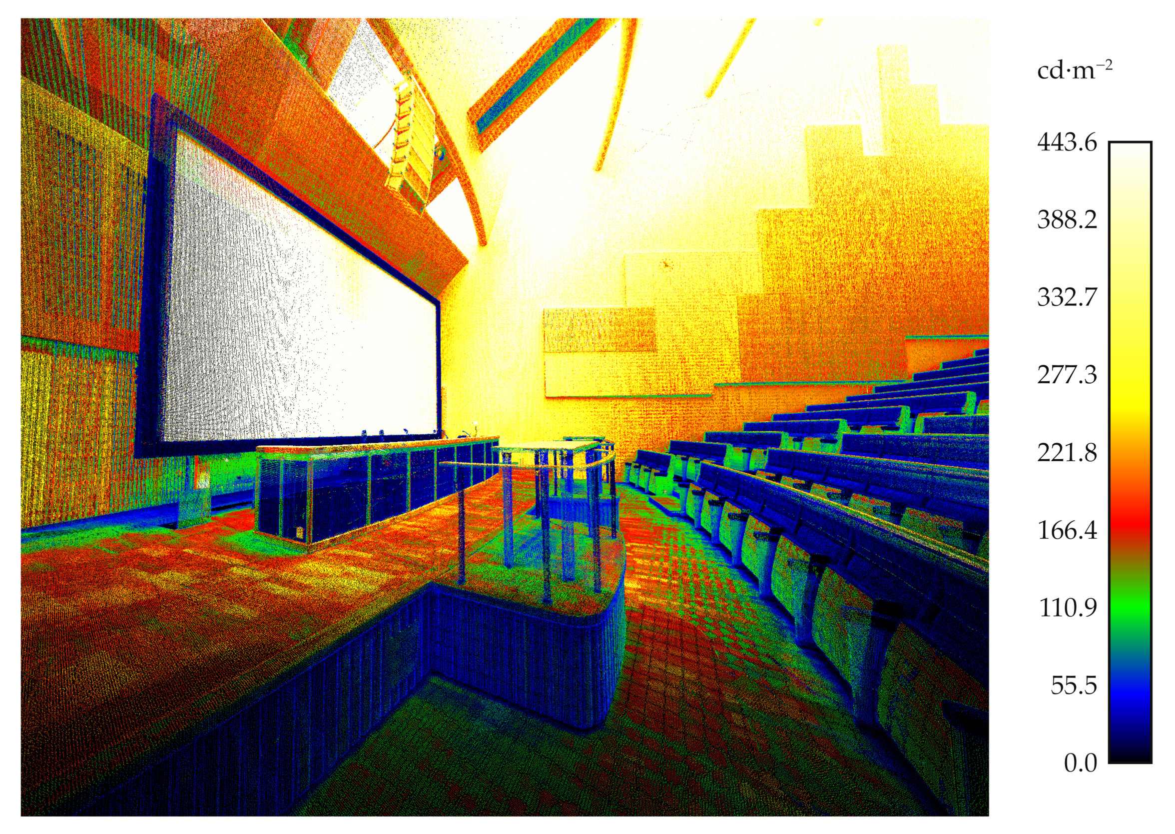
Figure 11.
The luminance point cloud of scanning station 2.
Figure 11.
The luminance point cloud of scanning station 2.
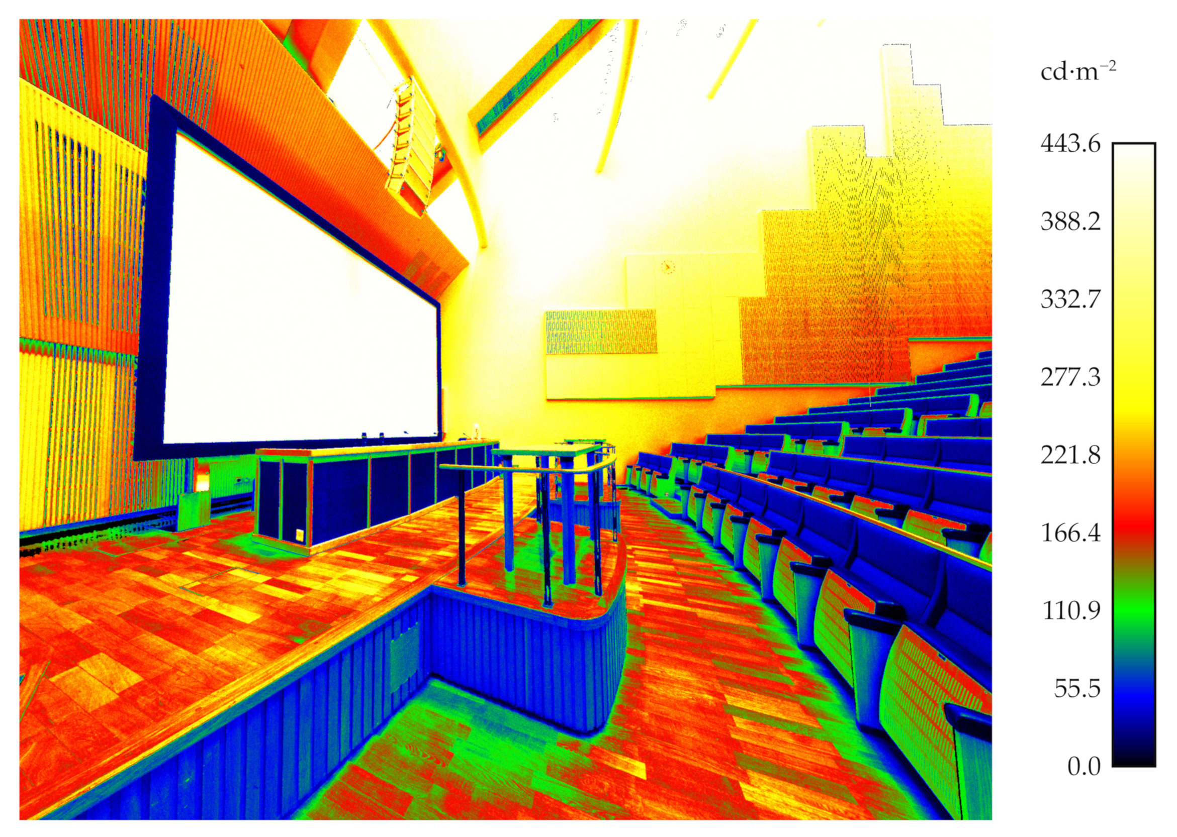
Figure 12.
The subsampled luminance point cloud of all scanning stations.
Figure 12.
The subsampled luminance point cloud of all scanning stations.
Figure 13.
The point cloud (a) and its corresponding histogram (b) for the vertical sample area, and the point cloud (c) and its corresponding histogram (d) for the horizontal sample area.
Figure 13.
The point cloud (a) and its corresponding histogram (b) for the vertical sample area, and the point cloud (c) and its corresponding histogram (d) for the horizontal sample area.
Table 1.
Measurements and results performed in the study and their sections.
Table 1.
Measurements and results performed in the study and their sections.
| Laboratory measurements | Method: | Reference color target measurements: (Section 2.2 Luminance calibration of a terrestrial laser scanner; Section 2.3 Luminance data processing) |
| | Results: | Luminance calibration factor for TLS: (Section 3.1 Reference color target measurements; Section 3.2 Luminance measurement comparison and Appendix A.1 Color target) |
| Field measurements | Method: | TLS data of the study area: (Section 2.4 Case study) and the luminance calibration factor from laboratory measurements |
| | Results: | Absolute luminance point clouds: (Section 3.3 Case study and Appendix A.2 Sample areas) |
Table 2.
The colorimetric reference data for the ColorChecker Classic chart provided by X-Rite. X-Rite No. is the patch name used by X-Rite; L is the luminance value; a and b are color coordinates.
Table 2.
The colorimetric reference data for the ColorChecker Classic chart provided by X-Rite. X-Rite No. is the patch name used by X-Rite; L is the luminance value; a and b are color coordinates.
| Patch No. | X-Rite No. | L | a | b |
|---|
| 1 | A4 | 95.19 | −1.03 | 2.93 |
| 2 | B4 | 81.29 | −0.57 | 0.44 |
| 3 | C4 | 66.89 | −0.75 | −0.06 |
| 4 | D4 | 50.76 | −0.13 | 0.14 |
| 5 | E4 | 35.63 | −0.46 | −0.48 |
| 6 | F4 | 20.64 | 0.07 | −0.46 |
| 7 | A3 | 28.37 | 15.42 | −49.8 |
| 8 | B3 | 54.38 | −39.72 | 32.27 |
| 9 | C3 | 42.43 | 51.05 | 28.62 |
| 10 | D3 | 81.8 | 2.67 | 80.41 |
| 11 | E3 | 50.63 | 51.28 | −14.12 |
| 12 | F3 | 49.57 | −29.71 | −28.32 |
| 13 | A2 | 62.73 | 35.83 | 56.5 |
| 14 | B2 | 39.43 | 10.75 | −45.17 |
| 15 | C2 | 50.57 | 48.64 | 16.67 |
| 16 | D2 | 30.1 | 22.54 | −20.87 |
| 17 | E2 | 71.77 | −24.13 | 58.19 |
| 18 | F2 | 71.51 | 18.24 | 67.37 |
| 19 | A1 | 37.54 | 14.37 | 14.92 |
| 20 | B1 | 64.66 | 19.27 | 17.5 |
| 21 | C1 | 49.32 | −3.82 | −22.54 |
| 22 | D1 | 43.46 | −12.74 | 22.72 |
| 23 | E1 | 54.94 | 9.61 | −24.79 |
| 24 | F1 | 70.48 | −32.26 | −0.37 |
Table 3.
The sample areas.
Table 3.
The sample areas.
| Sample Area | Material |
|---|
| A | wooden door |
| B | painted wood |
| C | painted concrete wall |
| D | painted vertical slatted timber |
| E | painted vertical slatted timber |
| F | painted horizontal slatted timber |
| G | painted concrete wall |
| Vertical | textile-covered acoustic board |
| Horizontal | wooden table |
Table 4.
The sRGB values (16-bit) of the X-Rite ColorChecker Classic board, calculated from the spectra measured with the spectroradiometer, and scaled to match the X-Rite nominal values.
Table 4.
The sRGB values (16-bit) of the X-Rite ColorChecker Classic board, calculated from the spectra measured with the spectroradiometer, and scaled to match the X-Rite nominal values.
| Patch No. | R | G | B |
|---|
| 1 | 62,782 | 62,269 | 56,751 |
| 2 | 41,236 | 41,525 | 38,895 |
| 3 | 25,391 | 25,701 | 23,993 |
| 4 | 13,472 | 13,375 | 12,370 |
| 5 | 6498 | 6633 | 6285 |
| 6 | 2699 | 2606 | 2414 |
| 7 | 2660 | 3735 | 20,103 |
| 8 | 4945 | 20,983 | 4284 |
| 9 | 29,753 | 3094 | 2760 |
| 10 | 57,323 | 40,884 | 285 |
| 11 | 35,392 | 6377 | 20,273 |
| 12 | −447 | 16,836 | 24,888 |
| 13 | 50,372 | 14,128 | 1888 |
| 14 | 4941 | 7354 | 26,861 |
| 15 | 38,649 | 6226 | 8016 |
| 16 | 7631 | 3249 | 9593 |
| 17 | 24,366 | 36,005 | 2981 |
| 18 | 53,556 | 26,190 | 1328 |
| 19 | 12,565 | 6284 | 4060 |
| 20 | 38,994 | 20,567 | 14,321 |
| 21 | 8588 | 13,919 | 22,313 |
| 22 | 7652 | 11,057 | 3514 |
| 23 | 16,275 | 14,978 | 28,129 |
| 24 | 9578 | 36,325 | 26,761 |
Table 5.
The laser scanner luminance measurements compared to a spectroradiometer. The table shows the differences and relative differences between the reference luminance measured with a spectroradiometer and the luminance measured with a TLS. The luminance measured with a TLS was calculated by linear regression and by linear regression and noise removal.
| Patch No. | A | B | C | Diff. (A,C) | Relative Diff. (A,C) | D | Diff. (A,D) | Relative Diff. (A,D) |
|---|
| 1 | 329.8 | 48,753.6 | 333.2 | 3.4 | 1.0% | 330.8 | 1.0 | 0.3% |
| 2 | 219.6 | 32,784.2 | 224.1 | 4.4 | 2.0% | 221.0 | 1.4 | 0.6% |
| 3 | 135.8 | 20,786.2 | 142.1 | 6.3 | 4.7% | 138.5 | 2.8 | 2.0% |
| 4 | 70.9 | 11,449.6 | 78.3 | 7.4 | 10.4% | 74.4 | 3.5 | 4.9% |
| 5 | 35.0 | 6165.6 | 42.1 | 7.1 | 20.4% | 38.1 | 3.0 | 8.7% |
| 6 | 13.9 | 2665.2 | 18.2 | 4.3 | 31.1% | 14.0 | 0.1 | 0.7% |
Table 6.
The consistency of images in five consecutive TLS scans.
Table 6.
The consistency of images in five consecutive TLS scans.
| Patch No. | #1 | #2 | #3 | #4 | #5 | avg | STD | RSD |
|---|
| 1 | 48,403 | 48,073 | 48,437 | 49,867 | 48,988 | 48,753.6 | 703.7 | 1.44% |
| 2 | 32,658 | 32,384 | 32,803 | 33,317 | 32,759 | 32,784.2 | 339.5 | 1.04% |
| 3 | 20,718 | 20,572 | 20,987 | 21,028 | 20,626 | 20,786.2 | 209.2 | 1.01% |
| 4 | 11,396 | 11,394 | 11,512 | 11,601 | 11,345 | 11,449.6 | 104.5 | 0.91% |
| 5 | 6144 | 6112 | 6180 | 6292 | 6100 | 6165.6 | 77.2 | 1.25% |
| 6 | 2638 | 2636 | 2680 | 2712 | 2660 | 2665.2 | 31.7 | 1.19% |
Table 7.
The relative luminance values calculated from the TLS 16-bit linear images compared to different sets of reference values. The table presents the values ordered according to the reference color target (
Figure 2).
Table 7.
The relative luminance values calculated from the TLS 16-bit linear images compared to different sets of reference values. The table presents the values ordered according to the reference color target (
Figure 2).
| TLS 16-Bit Linear Images Compared to the ReferenceValues Measured with a Spectroradiometer |
|---|
| Relative luminance values calculated from the TLS 16-bit linear images |
| 8418.6 | 24,482.7 | 15,137.8 | 10,691.0 | 17,647.0 | 31,555.7 |
| 19,673.6 | 10,007.0 | 13,167.5 | 5486.0 | 30,092.9 | 26,973.7 |
| 7559.0 | 18,091.8 | 37,820.5 | 37,820.5 | 13,644.1 | 17,318.7 |
| 61,969.5 | 41,645.5 | 14,543.5 | 14,543.5 | 7838.0 | 3379.1 |
| Linear spectroradiometer values calculated and scaled from the measured spectra |
| 7458.4 | 24,033.5 | 13,392.0 | 9788.6 | 16,203.3 | 29,948.3 |
| 20,950.0 | 8249.2 | 13,248.4 | 4638.9 | 31,146.1 | 30,213.0 |
| 4688.5 | 16,367.8 | 8737.3 | 41,447.7 | 13,549. | 13,742.7 |
| 61,979.3 | 41,273.9 | 25,512.0 | 13,322.6 | 6578.9 | 2611.9 |
| Relative difference between the values measured with a TLS and a spectroradiometer |
| 12.9% | 1.9% | 13.0% | 9.2% | 8.9% | 5.4% |
| 6.1% | 21.3% | 0.6% | 18.3% | 3.4% | 10.7% |
| 61.2% | 10.5% | 7.2% | 8.8% | 0.7% | 26.0% |
| 0.0% | 0.9% | 3.5% | 9.2% | 19.1% | 29.4% |
| | | | | Average: | 12.0
% |
Table 8.
The adjusted TLS luminance measurements compared to the reference values measured with a spectroradiometer. The table presents the values ordered according to the reference color target (
Figure 2).
Table 8.
The adjusted TLS luminance measurements compared to the reference values measured with a spectroradiometer. The table presents the values ordered according to the reference color target (
Figure 2).
| TLS Luminance Measurements Compared to the Reference Values Measuredwith a Spectroradiometer |
|---|
| Absolute adjusted luminance values measured with a TLS |
| 41.1 | 127.9 | 77.7 | 53.4 | 91.3 | 166.4 |
| 101.7 | 50.1 | 66.7 | 25.4 | 158.1 | 141.1 |
| 36.8 | 93.4 | 46.2 | 199.6 | 69.5 | 89.6 |
| 330.9 | 221.0 | 138.4 | 74.3 | 38.1 | 14.0 |
| Absolute adjusted luminance values measured with a spectroradiometer |
| 39.7 | 127.8 | 71.4 | 52.0 | 86.4 | 159.4 |
| 111.3 | 44.1 | 70.5 | 24.7 | 165.5 | 160.5 |
| 25.1 | 87.0 | 46.4 | 220.2 | 72.2 | 73.3 |
| 329.8 | 219.6 | 135.8 | 70.9 | 35.0 | 13.9 |
| Absolute difference |
| 1.5 | 0.1 | 6.4 | 1.4 | 5.0 | 7.1 |
| 9.6 | 6.0 | 3.7 | 0.7 | 7.4 | 19.4 |
| 11.7 | 6.4 | 0.3 | 20.6 | 2.7 | 16.3 |
| 1.1 | 1.3 | 2.7 | 3.4 | 3.1 | 0.1 |
| | | | | Average: | 5.7 |
| Relative difference |
| 3.7% | 0.1% | 8.9% | 2.7% | 5.8% | 4.4% |
| 8.6% | 13.7% | 5.3% | 2.8% | 4.5% | 12.1% |
| 46.7% | 7.4% | 0.6% | 9.3% | 3.7% | 22.3% |
| 0.3% | 0.6% | 2.0% | 4.9% | 8.8% | 0.4% |
| | | | | Average: | 7.5
% |
Table 9.
The vertical sample area: median luminance, Gaussian mean luminance, minimum luminance, maximum luminance, standard deviation, relative standard deviation, number of points, and angle between the surface normal and the measurement direction.
Table 9.
The vertical sample area: median luminance, Gaussian mean luminance, minimum luminance, maximum luminance, standard deviation, relative standard deviation, number of points, and angle between the surface normal and the measurement direction.
| No. | Lmedian | Lmean | Lmin | Lmax | LSTD | LRSD | Points | Angle |
|---|
| 1 | 243.0 | 242.2 | 198.1 | 279.7 | 11.0 | 4.5% | 10,066 | 26 |
| 2 | 346.6 | 345.7 | 278.3 | 402.0 | 13.8 | 4.0% | 9460 | 17 |
| 3 | 379.9 | 349.9 | 296.9 | 443.0 | 22.7 | 6.0% | 10,184 | 66 |
| 4 | 358.7 | 358.2 | 314.7 | 411.7 | 12.9 | 3.6% | 8310 | 59 |
| 5 | 334.7 | 334.3 | 283.8 | 388.9 | 15.6 | 4.7% | 3537 | 69 |
| 6 | 299.4 | 300.0 | 265.9 | 341.4 | 10.9 | 3.6% | 6273 | 36 |
| 7 | 353.8 | 353.4 | 300.9 | 407.9 | 13.9 | 3.9% | 8805 | 18 |
| All | 346.3 | 330.7 | 198.1 | 443.0 | 48.9 | 14.8% | 56,635 | 17–69 |
| Allsubsampled | 346.5 | 331.1 | 198.1 | 442.9 | 49.7 | 15.0% | 9295 | 17–69 |
Table 10.
The horizontal sample area: median luminance, Gaussian mean luminance, minimum luminance, maximum luminance, standard deviation, relative standard deviation, number of points, and angle between the surface normal and the measurement direction. Scans 2 and 3 were left with no observations due to the large measurement angle.
| No. | Lmedian | Lmean | Lmin | Lmax | LSTD | LRSD | Points | Angle |
|---|
| 1 | 244.9 | 244.4 | 194.8 | 346.3 | 14.4 | 5.9% | 7374 | 63 |
| 2 | - | - | - | - | - | - | - | 87 |
| 3 | - | - | - | - | - | - | - | 88 |
| 4 | 369.5 | 369.7 | 311.6 | 410.0 | 12.4 | 3.4% | 3617 | 81 |
| 5 | 310.2 | 310.0 | 266.0 | 356.7 | 13.0 | 4.2% | 2264 | 76 |
| 6 | 367.5 | 367.9 | 315.2 | 419.5 | 14.4 | 3.9% | 2620 | 76 |
| 7 | 428.1 * | 427.9 * | 399.1 * | 443.5 * | 5.1 * | 1.2% * | 6336 | 79 |
| All | 302.6 | 302.7 | 194.8 | 419.5 | 59.2 | 19.5% | 15,875 | 63–88 |
| Allsubsampled | 257.3 | 284.2 | 194.8 | 419.5 | 54.4 | 19.1% | 10,367 | 63–88 |
Table 11.
The sample areas A–G: median luminance, Gaussian mean luminance, minimum luminance, maximum luminance, standard deviation, relative standard deviation, number of points, and angle between the surface normal and the measurement direction.
Table 11.
The sample areas A–G: median luminance, Gaussian mean luminance, minimum luminance, maximum luminance, standard deviation, relative standard deviation, number of points, and angle between the surface normal and the measurement direction.
| Sample Area | Lmedian | Lmean | Lmin | Lmax | LSTD | LRSD | Points | Angle |
|---|
| A | 90.7 | 89.3 | 44.0 | 128.8 | 14.0 | 15.7% | 8468 | 16–69 |
| B | 194.3 | 192.5 | 98.0 | 255.0 | 26.2 | 13.6% | 13,247 | 11–51 |
| C | 369.2 | 369.3 | 277.9 | 443.4 | 35.2 | 9.5% | 9376 | 18–63 |
| D | 159.0 | 165.5 | 42.3 | 336.4 | 60.9 | 36.8% | 20,158 | 11–79 |
| E | 268.3 | 268.1 | 117.0 | 430.9 | 56.3 | 21.0% | 19,172 | 9–65 |
| F | 178.6 | 174.4 | 105.0 | 233.2 | 24.3 | 14.0% | 12,208 | 15–65 |
| G | 231.2 | 223.9 | 150.6 | 276.9 | 29.3 | 13.1% | 9836 | 14–63 |
| Vertical | 346.5 | 331.1 | 198.1 | 442.9 | 49.7 | 15.0% | 9295 | 17–69 |
| Horizontal | 257.3 | 284.2 | 194.8 | 419.5 | 54.4 | 19.1% | 10,367 | 63–88 |


 ,
, 


